Multistate hybrid time-dependent density functional theory with surface hopping accurately captures ultrafast thymine photodeactivation
Received
3rd June 2019
, Accepted 6th August 2019
First published on 29th August 2019
Abstract
We report an efficient analytical implementation of first-order nonadiabatic derivative couplings between arbitrary Born–Oppenheimer states in the hybrid time-dependent density functional theory (TDDFT) framework using atom-centered basis functions. Our scheme is based on quadratic response theory and includes orbital relaxation terms neglected in previous approaches. Simultaneous computation of multiple derivative couplings and energy gradients enables efficient multistate nonadiabatic molecular dynamics simulations in conjunction with Tully's fewest switches surface hopping (SH) method. We benchmark the thus obtained multistate TDDFT-SH scheme by simulating ultrafast decay of UV-photoexcited thymine, for which accurate gas-phase data from ultrafast spectroscopy experiments are available. The calculations predict a fast 153 fs decay from the bright S2 to the dark S1 excited state, followed by a much slower 14 ps S1 deactivation to the ground state; statistical uncertainties were estimated using bootstrap sampling. These results agree well with the experimentally observed time constants of 100–200 fs and 5–7 ps, respectively, unlike previous multiconfigurational self-consistent field and second-order algebraic diagrammatic construction calculations. Furthermore, our results support the S1-trapping hypothesis [J. J. Szymczak et al., J. Phys. Chem. A, 2009, 113, 12686–12693]. For thymine, the computational cost of a single TDDFT-SH time-step including the lowest 3 states, all couplings and gradients, is ∼5 times larger than the cost of a single Born–Oppenheimer dynamics time step for the ground state in our implementation. Thus, ps nonadiabatic dynamics simulations using multistate hybrid TDDFT-SH for systems with up to ∼100 atoms are possible without drastic approximations on single workstation nodes. Our implementation will be made available through Turbomole.
1 Introduction
Nonadiabatic molecular dynamics1 (NAMD) using a combination of time-dependent density functional theory2–7 (TDDFT) and surface hopping8 (SH) has emerged as a versatile tool for studying and analyzing complex photochemical transformations.9–11 TDDFT-SH has proven capable of predicting the kinetics of pericyclic ring-opening and -closing reactions,12–20 the reactivity of photoexcited metal oxides21 such as perovskites22 and titania,23–25 and the branching ratios, kinetic energy distributions, and mass distributions of photodissociation reactions.26,27
However, the majority of photochemical TDDFT-SH applications to date have included only the ground state and the first excited state. Simulations including several excited states and all nonadiabatic couplings between them have been reported, but rely on approximations with questionable validity such as the neglect of orbital relaxation17,19,28–32 or single Slater determinant models for the excited state. A rigorous theoretical approach to general couplings between excited states in the TDDFT framework has only recently been devised,33–35 but little is known about its performance in photochemical applications.
Here we report an efficient analytical implementation of state-to-state nonadiabatic couplings and multistate TDDFT-SH dynamics, which builds on these theoretical results and the implementation of the TDDFT quadratic response properties reported by our group previously.36 All required gradients and couplings can be computed simultaneously; as a result, the computational cost for a multistate NAMD time-step is proportional to that of a ground-state Born–Oppenheimer dynamics step, with a proportionality constant growing sublinearly with the number of electronic states.
We assess the performance of multistate TDDFT by investigating excited state decay of UV-photoexcited thymine. The experimental lifetime of UV-photexcited thymine, 5–7 ps, is significantly longer than that of other photoexcited nucleobases,37 and its decay has been extensively studied experimentally37–44 and computationally.43,45–53 Nevertheless, the deactivation mechanism of UV-photoexcited thymine remains controversial.37,45,53 In particular, prior NAMD-SH simulations using multiconfiguration self-consistent field (MCSCF) and the second-order algebraic diagrammatic construction [ADC(2)] methods lead to excited-state lifetimes hard to reconcile with each other and with ultrafast pump–probe experiments.37,43,50,52
We summarize the working equations and details of our implementation in Sections 2 and 3, followed by the results for thymine excited-state deactivation in Section 4 and conclusions in Section 5.
2 Nuclear dynamics: fewest switches surface hopping
Mixed quantum-classical methods treat nuclei classically and expand an auxiliary electronic wavefunction in a few-state (often adiabatic) electronic basis parametrically dependent on the nuclear coordinates.8 In our implementation, the auxiliary electronic density matrix| | 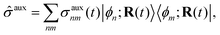 | (1) |
is the basic dynamic variable, where R(t) denotes the nuclear coordinates, σauxnm(t) are expansion coefficients at time t, and ϕn are electronic basis states.8,54,55 The auxiliary electronic density matrix evolves as| | 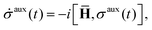 | (2) |
where ![[H with combining macron]](https://www.rsc.org/images/entities/b_char_0048_0304.gif) = H − iW is the effective Hamiltonian, Hnm = 〈ϕn;R(t)|Ĥ|ϕm;R(t)〉 is a matrix element of the electronic Hamiltonian,
= H − iW is the effective Hamiltonian, Hnm = 〈ϕn;R(t)|Ĥ|ϕm;R(t)〉 is a matrix element of the electronic Hamiltonian,| |  | (3) |
is a nonadiabatic coupling matrix element and| |  | (4) |
is the first-order derivative coupling between electronic states n and m.8
Within surface hopping, the electronic properties for a given trajectory at any give time are determined by a single Born–Oppenheimer electronic state, here referred to as the active state or active surface.54 This picture implicitly defines an active electronic density matrix,
where
k labels the active electronic state. Transitions between electronic states are mimicked through stochastic hops of the active state.
FSSH is a specific realization of the surface hopping framework in which the probability of hopping from active state k to electronic state n in the time interval t to t′,
| |  | (6) |
is chosen to reproduce the swarm average population of state
k—that is, so
Nk(
t)/
Ntraj ≈
σkk(
t) where
Nk(
t) is the number of trajectories on active surface
k and
Ntraj is the total number of trajectories.
8 In practice, surface hops are decided by computing hopping probabilities according to
eqn (6) and generating a uniform random number
η ∈ [0,1]. When
η <
gk→n, a surface hop to state
n is initiated and the momentum along the derivative coupling vector is rescaled to conserve energy.
8 In case of insufficient kinetic energy,
i.e. a frustrated hop, the hop is rejected and no momentum readjustment is performed.
3 Electronic dynamics: TDDFT
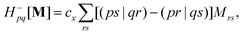
The NAMD frameworks described above require as input the adiabatic energies of electronic states (En), nuclear forces (∇En), and derivative couplings (τ(ξ)nm ≡ 〈ϕn|∇ξϕm〉). All of these quantities are computed using (TD)DFT: ground state properties are determined from ground state DFT, excitation energies and derivative couplings between the ground state and an excited electronic state (ground-to-excited-state) are determined from linear response, and excited-state forces and derivative couplings between two excited electronic states (state-to-state) are determined from the quadratic response function.
3.1 Linear response
In the TDDFT linear response framework,2–4,56,57 excitation energies are obtained by solving the eigenvalue problemwhere| |  | (8) |
is the linear response operator;| | | (A + B)ia,jb = εabδij − εijδab + 2fxcia,jb + 2(ia|jb) − cx[(ib|ja) + (ij|ab)] | (9a) |
| | | (A − B)ia,jb = εabδij − εijδab + cx[(ib|ja) − (ij|ab)], | (9b) |
denote the electronic and magnetic orbital rotation Hessians, respectively;| |  | (10) |
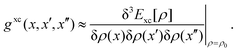
is the pseudometric, and Ωn and |Xn,Yn〉 are the eigenvalue (excitation energy) and associated eigenvector of excited state n, respectively.4,56 Here, indices i, j,… denote occupied, a, b,… virtual, and p, q,… general Kohn–Sham molecular orbitals. Moreover, εpq is an element of the Kohn–Sham matrix which is assumed to be block-diagonal (i.e., the occupied–virtual blocks vanish), fxcpq,rs is an element of the exchange–correlation kernel, (pq|rs) is an element of the Coulomb operator in Mulliken notation, and cx is a scalar that interpolates between pure semilocal density functionals (cx = 0) and Hartree–Fock theory (cx = 1, fxc = 0). The vast majority of applications use the adiabatic approximation,58 which replaces the frequency-dependent exchange–correlation kernel with its static limit. The excitation vector for state n encodes the Kohn–Sham ground-to-excited state transition density matrix| |  | (11) |
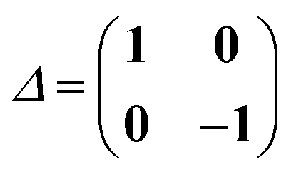
in terms of the Kohn–Sham orbitals φp.57 Eigenvectors of eqn (7) satisfy the orthonormalization condition| | | 〈Xn,Yn|Δ|Xm,Ym〉 = δnm. | (12) |
3.2 Ground-to-excited-state derivative couplings
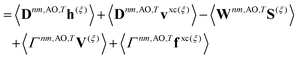
First-order derivative couplings between the ground and an excited electronic state within the adiabatic approximation to TDDFT are obtained from a pole analysis of the frequency-dependent linear response of the time-dependent Kohn–Sham wavefunction,33,59 and are computed together with excited-state gradients as| | | τ(ξ)0n = 〈D0n,AOh(ξ)〉 + 〈D0n,AOvxc,(ξ)〉 − 〈W0n,AOS(ξ)〉 + 〈Γ0n,AOV(ξ)〉; | (13) |
here, the superscript (ξ) indicates partial differentiation, ξ represents the nuclear coordinate of interest, the superscript MAO ≡ CMC† indicates the quantity is expressed in the AO basis for molecular orbital coefficient matrix C, h is the one-electron core Hamiltonian, vxc is the exchange–correlation potential, S is the overlap matrix, D0n is a generalized one-electron transition density, W0n is a generalized energy-weighted transition density, Γ0n is the pair transition density, and V is the two-electron Coulomb operator defined with Vμνλκ = (μν|λκ); greek indices denote AOs. At variance with ref. 59, we include in eqn (13) only translationally invariant terms, which is approximately equivalent to employing electron-translation factors.60,61
3.3 State-to-state derivative couplings
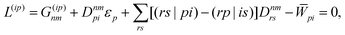
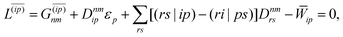
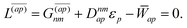
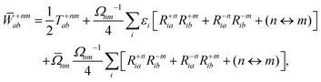
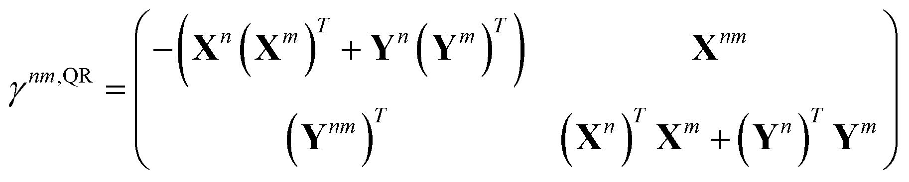
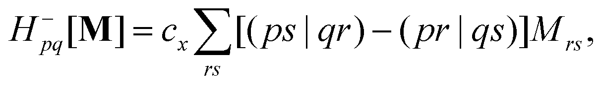
In analogy to the ground-to-excited state derivative couplings, state-to-state derivative couplings are defined through a pole analysis of the quadratic response function. The generator for the derivative coupling between excited states n and m is33| | | Gnm(C,ε|γnm,R) = 〈Xn,Yn|Λ(R)|Xm,Ym〉/Ωnm + 〈γnm,TC(0)†O(R)C〉, | (14) |
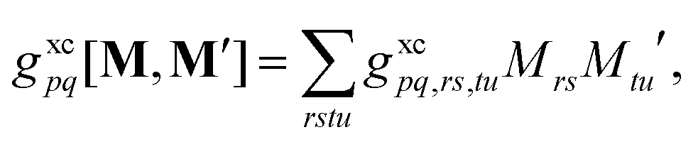
where Oμν(R) ≡ 〈χμ|χν(R)〉 is a one-sided atomic orbital overlap integral, |χμ〉 is an atom-centered Gaussian basis function, the superscript (0) indicates that the quantity is fixed at the zeroth-order solution, Ωnm ≡ Ωn − Ωm, γnm is the 1-particle transition density matrix (1TDM) of the KS system, and dependence on the nuclear coordinates, R, is now denoted explicitly.
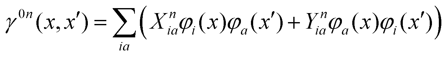
Quadratic response theory dictates that the 1TDM in eqn (14) is obtained from
| |  | (15) |
where the off-diagonal blocks require the solution of a dynamic-polarizability-like equation,
| | | |Xnm,Ynm〉 = −(Λ − ΩnmΔ)−1|Pnm,Qnm〉 | (16) |
Explicit expressions for the right-hand-side (RHS) are provided in
ref. 36 and supplied in the Appendix for completeness. However, within the adiabatic approximation to the exchange–correlation kernel, the linear response operator in
eqn (16) becomes singular when
Ωnm approaches any other excitation energy and thus the transition density diverges unphysically.
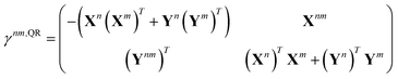
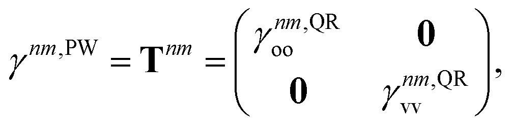
33–36,62 Thus, we exclusively use derivative couplings from the pseudowavefunction approximation which is equivalent to ignoring the off-diagonal blocks of the 1TDM in
eqn (14),
| |  | (17) |
where
γnm,QRoo and γ
nm,QRvv are the occupied–occupied and virtual–virtual blocks of
γnm,QR, and
Tnm is referred to as the unrelaxed 1TDM.
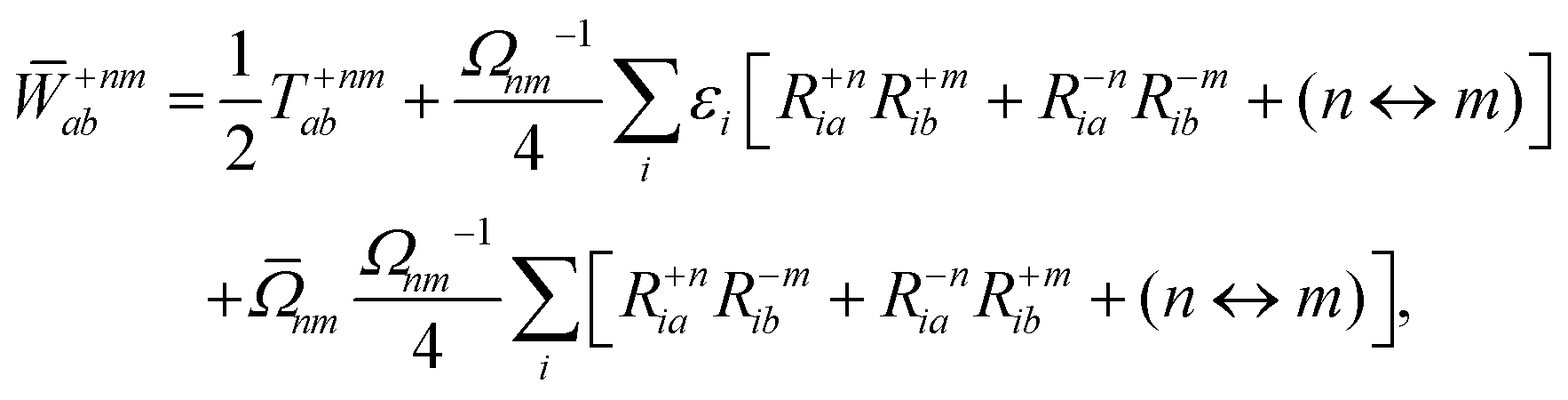
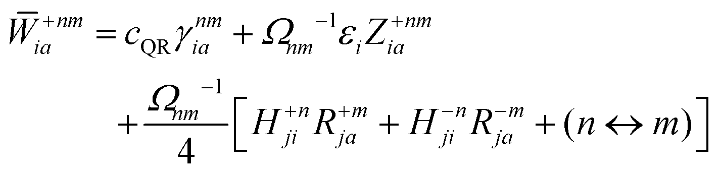
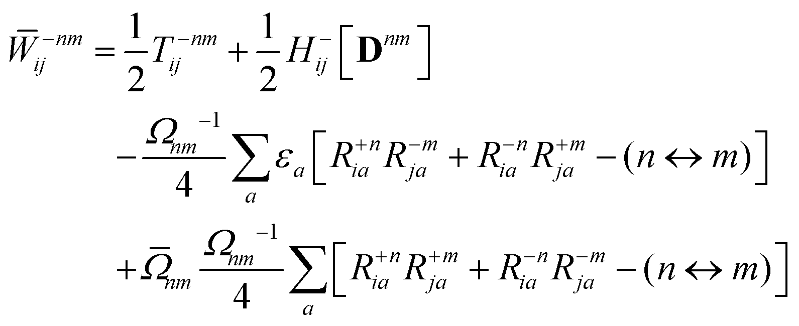
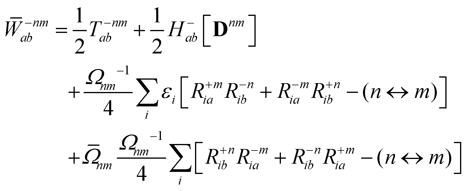
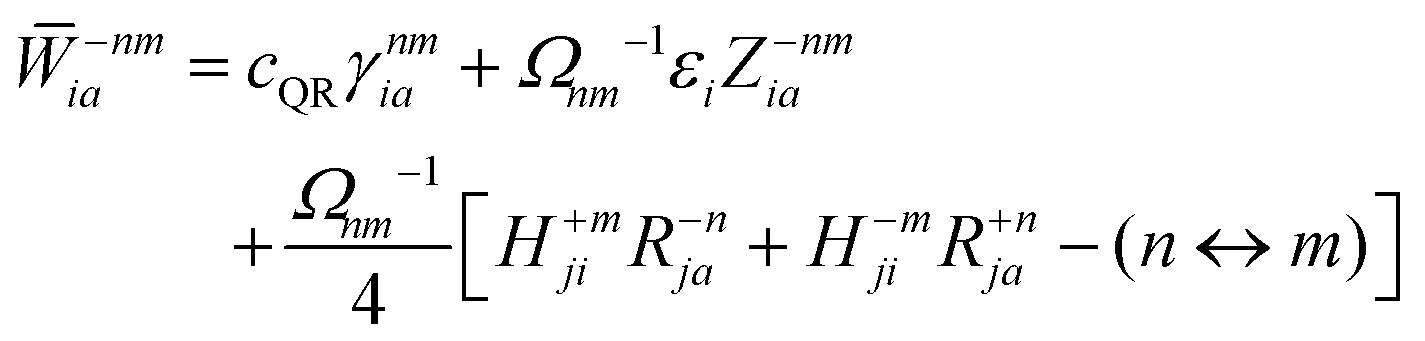
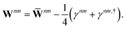
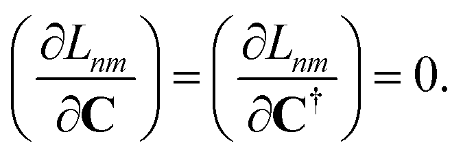
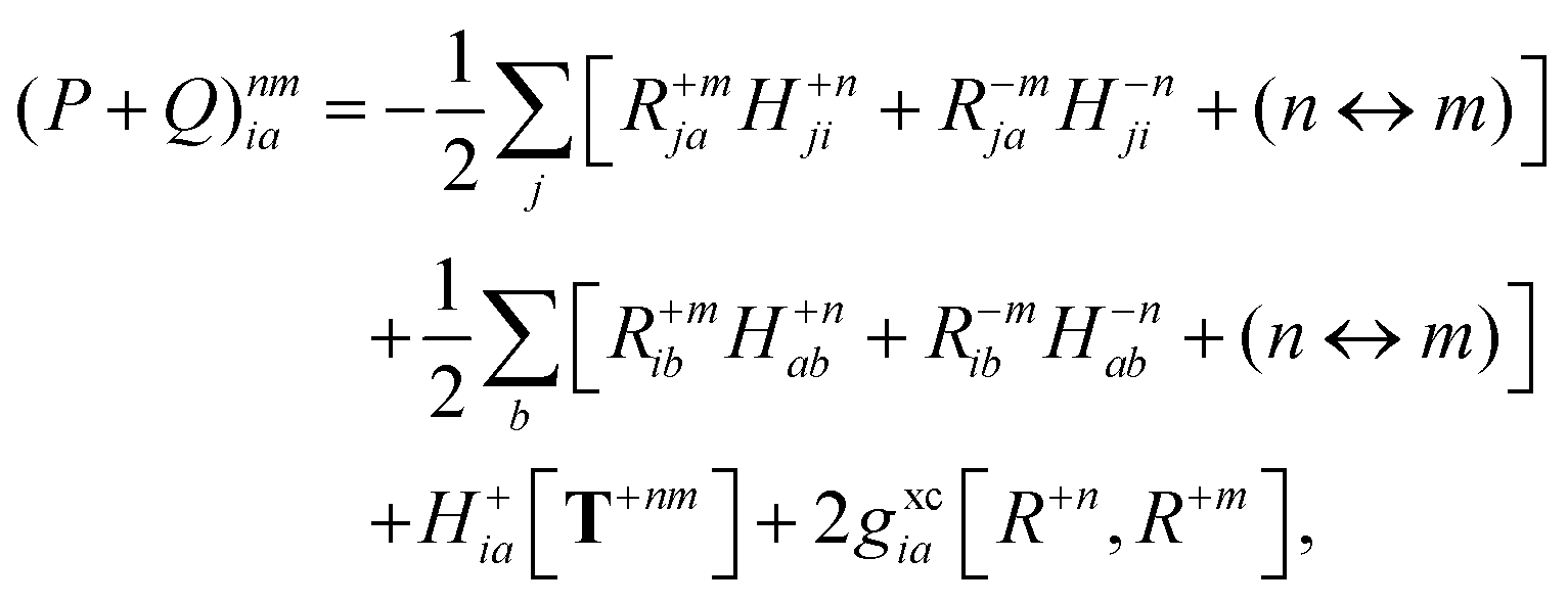
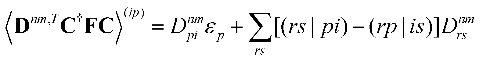
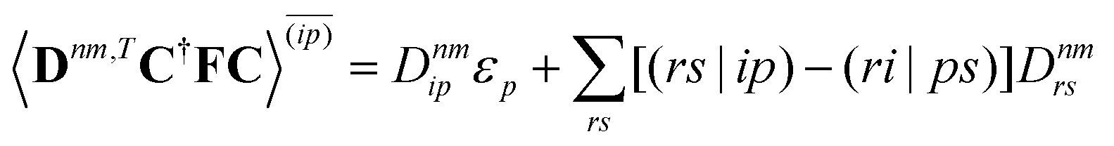
Regardless of the choice of 1TDM in eqn (14), an expression for the state-to-state derivative couplings including all Pulay terms is obtained by stationarizing the Lagrangian
| | Lnm[C,ε,Dnm,![[W with combining macron]](https://www.rsc.org/images/entities/b_char_0057_0304.gif) nm] = Gnm(C,ε|γnm,R) + 〈Dnm,T(C†FC − ε)〉 − 〈nm,T(C†SC − I)〉 nm] = Gnm(C,ε|γnm,R) + 〈Dnm,T(C†FC − ε)〉 − 〈nm,T(C†SC − I)〉 | (18) |
where
ε is a Lagrange multiplier assumed to be block-diagonal,
F is the (density-matrix dependent) Fock matrix in atomic orbital (AO) representation,
Dnm and
nm are Lagrange multipliers that require the molecular orbitals to satisfy the KS equation and enforce orthonormality, respectively, and 〈·〉 indicates a trace.
Dnm and
nm are determined by enforcing stationarity with respect to the remaining parameters,
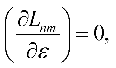
| |  | (19) |
and
| |  | (20) |
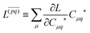
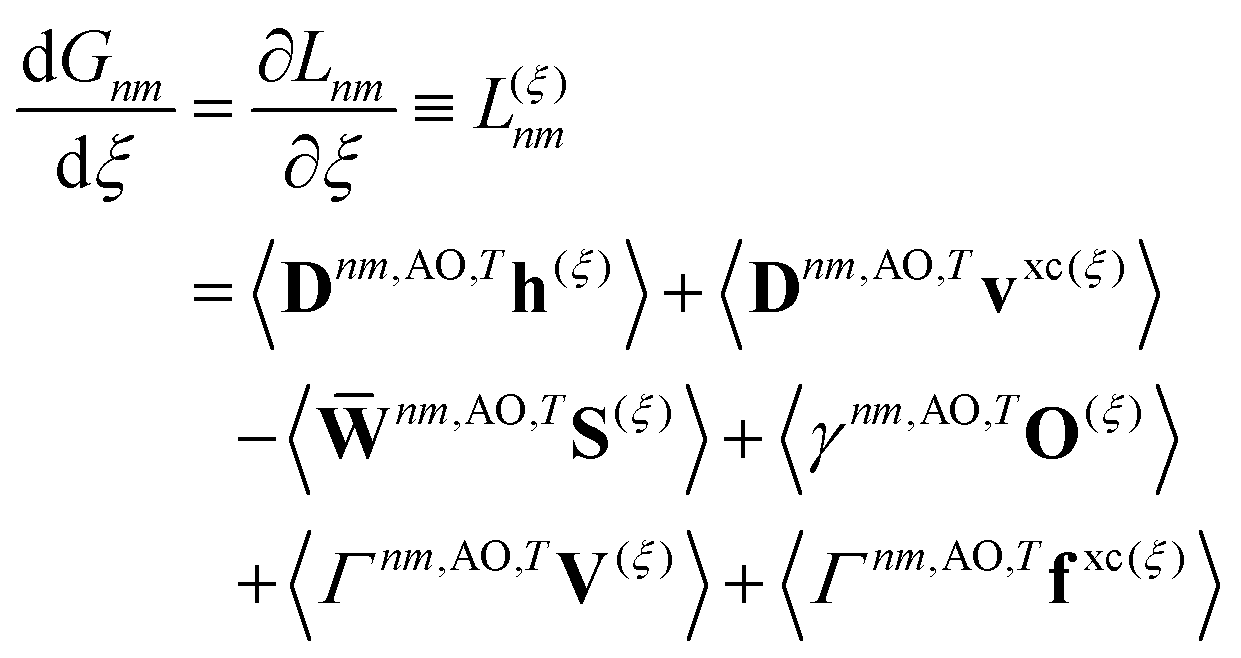
Real orbitals are assumed only after taking derivatives such that fully general expressions are obtained. An outline of the derivation is provided in the Appendix. At the stationary point, the total derivative of
Gnm is obtained straightforwardly through a partial derivative of the Lagrangian,
| | 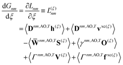 | (21) |
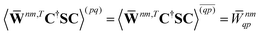
| |  | (22) |
where
Γnm is the pair transition density and all other quantities are defined as in
eqn (13).
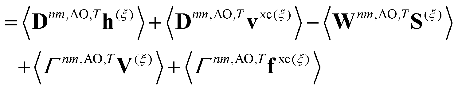
Eqn (22) follows from
eqn (21) by introducing
S(−ξ)μν = 〈
χ(ξ)μ|
χν〉 − 〈
χμ|
χ(ξ)ν〉, then recognizing that
O(ξ) = ½(
S(ξ) +
S(−ξ)) such that the Hermitian part of
γnm can be combined with
nm,
| |  | (23) |
The contractions involving
S(−ξ) with the anti-Hermitian part of
γnm can be neglected on physical grounds.
60
3.4 State-to-state derivative coupling implementation
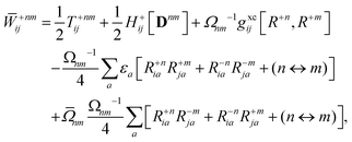
Eqn (22) was implemented into the program  ,63 building on the existing implementation of excited-state gradients and ground-to-excited-state derivative couplings. The rate-determining steps are the computation of a user-specified set of excitations, eqn (7), the construction of the relaxed densities, eqn (16), and the final contraction of the effective densities with operator partial derivatives, eqn (22). First, a user-specified set of excited states are computed, then couplings are computed between all excitations in a user-specified subset of the original excitations. For each pair of excited states, one coupled-perturbed Kohn–Sham (CPKS) calculation is required (for derivative couplings within full quadratic response theory, this becomes a dynamic polarizability calculation). The right-hand-sides for all pairs of excited states in eqn (16) are computed simultaneously, together with the right-hand-sides for excited-state gradients,63 using identical methodology as excited-state absorption calculations.36 Thus the state-to-state derivative coupling implementation achieves the same high resource-efficiency as shown for other quadratic response properties,36 up to the final contraction with operator derivatives. The required CPKS calculations were performed iteratively and simultaneously as described in ref. 36 and 64 with an integral driven65–69 nonorthonormal Krylov space block Davidson algorithm.70 Finally, for each operator type (e.g., h), contractions between its partial derivatives (h(ξ)) and all effective densities—including effective densities needed to compute ground- and excited-state gradients—were performed together such that the partial derivatives only need to be computed once.
Our implementation permits the computation of derivative couplings between excited-states computed with spin-restricted Kohn–Sham (RKS) or spin-unrestricted KS (UKS) orbitals, with or without the resolution-of-the-identity approximation for the Coulomb integrals,71 with and without applying the Tamm–Dancoff approximation,72 and for non-hybrid and hybrid semilocal density functionals, or time-dependent Hartree–Fock. Transition densities and RHSs between excited states were verified by reconstructing the dynamic hyperpolarizability from the exact TDDFT sum-over-states expressions. The final derivative couplings were verified against finite difference results.33
4 Excited-state deactivation of thymine
4.1 Prior results
Experimentally, three decay channels of UV-photoexcited thymine have been distinguished on the basis of gas phase femtosecond pump–probe transient ionization spectroscopy,37,38,40–43 femtosecond time-resolved photoelectron spectroscopy (TRPES),39 and ultrafast X-ray Auger,44 see Table 1: (i) a prompt signal with a time constant near 100–200 fs (ii) a fast signal with time constant of 5.1–7 ps and (iii) a slow decay conventionally attributed to intersystem crossing that is longer than 100 ps. Although mechanistic details could be inferred for aqueous thymine photodynamics using UV resonance Raman spectroscopy,73,74 the decay mechanism of UV-photoexcited thymine in the gas phase is experimentally difficult to probe.
Table 1 Summary of experimental time constants for ultrafast deactivation of UV-photoexcited thymine37–42 obtained with experimental techniques pump–probe transient ionization (PPTI), pump–probe resonant ionization (PPRI), pump–probe ionization spectroscopy (PPIS), and time-resolved photoelectron spectroscopy (TRPES)
| Measurement |
Component |
| Ultrashort (fs) |
Prompt (fs) |
Fast (ps) |
Slow (ns) |
| PPTI37 |
|
|
6.4 |
>100 |
| TRPES39 |
<50 |
490 |
6.4 |
|
| PPRI38 |
|
105 |
5.12 |
|
| PPIS40,41 |
|
130 |
6.5 |
|
| PPIS42 |
|
100 |
7 |
>1 |
| X-ray Auger44 |
|
200 |
|
|
The photodynamics of nucleic acids and nucleobases have been studied extensively computationally53 using a range of different approaches, including characterization of the minimum energy pathways through conical intersections42,46,47,75,76 and direct dynamics simulations.43,48–52 Here, we focus on on-the-fly dynamical simulations of photoexcited thymine and refer the interested reader to a several extensive reviews for additional details.45,53 Previously reported on-the-fly simulations of thymine photodynamics can be broadly categorized according to the electronic structure methods used to power the dynamics, see Table 2. To date, the most advanced on-the-fly NAMD simulations have used semiempirical models,77 MCSCF,43,49–51 and ADC(2) theory, with partially conflicting conclusions.
Table 2 Summary of computed time constants for ultrafast deactivation of UV-photoexcited thymine with available confidence intervals shown in parentheses in comparison to experimental results (see Table 1 for details)
| Method |
Component |
| Prompt |
Assignment |
Fast |
Assignment |
| Semiempirical48 |
420 fs |
S1 → S0 |
|
S0 → S0,eq |
| CASSCF43,49–51 |
100–200 fs |
S2,FC → S2,min |
2.6–5 ps |
S2,min → S1 |
| ADC(2)52 |
250 fs |
S2 → S1 |
420 fs |
S1 → S0 |
| PBE0/SVP (this work) |
153 fs (147–162 fs) |
S2 → S1 |
13.9 ps (10.4–21 ps) |
S1 → S0 |
| PBE0/SVPD (this work) |
110 fs (82–128 fs) |
S2 → S1 |
20.5 ps (11.6–49 ps) |
S1 → S0 |
|
|
| Exp. |
100–200 fs |
|
5–7 ps |
|
In particular, there appears to be no general consensus on the deactivation mechanism for photoexcited thymine with an excitation wavelength of 266 nm, near absorption onset. Semiempirical models such as multireference configuration interaction with the OM2 Hamiltonian77 (OM2/MRCI)—which are parametrized to reproduce energies near ground state geometries and can thus become unreliable far from the Franck–Condon region such as near conical intersections—predict an overall excited-state lifetime of 437 fs, about one order of magnitude faster than that observed experimentally.48 Furthermore, the predicted S2 lifetime of 17 fs and S1 lifetime of 420 fs lead to the interpretation that the ultrashort signal corresponds to internal conversion S2 → S1, the prompt signal corresponds to internal conversion to the ground state (S1 → S0) and the fast component corresponds to thermalization on the ground state.48
MCSCF, especially the state-averaged complete active space self-consistent field (SA-CASSCF) variant, is commonly used for NAMD simulations because, as a multireference method, it correctly recovers the topology of potential energy surface crossings.78 However, CASSCF lacks dynamical correlation and can therefore overestimate the absorption onset and the S2–S1 energy gap by up to 1.5 eV in thymine relative to more accurate methods.51 Thymine's photochemistry has been simulated using CASSCF by several different groups43,49–51 with a qualitatively consistent picture emerging in which photoexcited thymine relaxes from the Franck–Condon (FC) geometry to a minimum on the S2 potential energy surface with a time constant of 100–200 fs thus giving rise to the prompt signal. The S2 state then decays to the S1 state with an estimated time constant of 2.6–5 ps and S1 also exhibits a lifetime of several ps although precise estimates have not been provided. From this, the fast signal is assigned to the compound S2,min → S1 → S0 deactivation. The relatively long S2 lifetime has been attributed to a small but significant energetic barrier of ≈0.25 eV (5.7 kcal mol−1) between the S2 minimum and the S2/S1 conical intersection.75 However, this trapping on the S2 state surface was called into question based on ultrafast X-ray Auger experiments that observe a distinct electronic relaxation within 200 fs.44 Furthermore, the barrier all but disappears with the inclusion of dynamic correlation. For example, the barrier falls to 0.05 meV (1 kcal mol−1) using multistate complete active-space second-order perturbation theory (MS-CASPT2).75
To test the effect of dynamic correlation on the ensuing dynamics, Stojanović et al.52 used the ADC(2) method. ADC(2) is complementary to CASSCF in that dynamic correlation is explicitly included to second-order, but being a single-reference method, ADC(2) is sensitive to strong static correlation due to near-degeneracy of the ground state. In particular, although state-to-state conical intersections are correctly reproduced, ground-to-excited-state intersections have the wrong dimensionality.79 However, this may not be a cause for concern; preliminary investigations have shown that mixed quantum-classical trajectories are relatively insensitive to the dimensionality of the surface crossing, producing qualitatively similar results for different excited-state surface topologies.80 As opposed to the several picosecond S2 lifetime found with CASSCF dynamics, ADC(2) based dynamics indicate that following relaxation to the S2 minimum in 100 fs, the majority of trajectories (84%) decay to S1 within 250 fs. Out of these trajectories, 83% (70% of total trajectories) decay to the ground state within 400 fs. This lead to the conclusion that the prompt signal corresponds to decay to S2 with the fast signal corresponding to S1 → S0 deactivation, but the computed rate for the latter reaction is approximately one order of magnitude too fast.
4.2 Computational details
Initial conditions were drawn randomly from a 9.5 ps ground state ab initio molecular dynamics (AIMD) simulation at 500 K after a 0.5 ps equilibration period. The molecular dynamics were propagated with the leapfrog Verlet algorithm with an 80 a.u. (≈1.935 fs) time step. The TPSS density functional81 with D3 dispersion corrections82 and Becke–Johnson (BJ) damping parameters83 and the def2-SVP basis set84 was used to compute the ground state energy at each time step. For these AIMD simulations, the resolution-of-the-identity (RI) was used to approximate the two-electron Coulomb integrals,71 m3 grids with quadrature weight derivatives were used for functional integrations, and self-consistent field (SCF) convergence thresholds were set to 10−7Eh ( ).
).
NAMD simulations were initiated on the bright S2 surface with initial electronic density matrix σnm = δn,2δm,2 and used the PBE0 density functional85 with D3-BJ dispersion corrections82,83 and either split valence (def2-SVP)84 or property-optimized (def2-SVPD)86 basis sets. Excited states were computed within the Tamm–Dancoff approximation (TDA).72 Molecular dynamics were propagated with the leapfrog Verlet algorithm and a time step of 40 a.u. (0.9676 fs). For the NAMD simulations, size 4 grids with quadrature weight derivatives were used for functional integrations, SCF convergence thresholds were set to 10−9Eh ( ), and excited states were converged to a residual norm of less than 10−7 (
 ). As for ADC(2), conical intersections between the ground state and an excited state have incorrect dimensionality with TDDFT.78 To avoid potential associated instabilities, trajectories are forced to hop to the ground state if the first excitation energy, Ω1, falls below 0.5 eV. In total, we simulated 200 independent trajectories for a combined 650 ps of simulation time.
All uncertainties indicated here correspond to 95% confidence intervals (CI) estimated from bootstrap sampling with 10![[thin space (1/6-em)]](https://www.rsc.org/images/entities/char_2009.gif) 000 samples.87 Bootstrap sampling is a powerful resampling technique to estimate uncertainties in properties computed from a set of measurements of a stochastic process, i.e., without assuming an analytical distribution. Bootstrap sampling is therefore well-suited to estimating errors from NAMD trajectories where no information about the underlying statistical process is available.88 To obtain the bootstrap confidence interval of, for example, the mean value of a given set of Nmeasure measurements of a stochastic process, Nbootstrap replica samples are generated, the mean is computed for each replica sample, and confidence intervals are chosen to compactly contain the specified proportion of all replica means. Replica samples are generated by randomly selecting Nmeasure measurements with replacement (meaning duplicates are likely) out of the original Nmeasure measurements.
000 samples.87 Bootstrap sampling is a powerful resampling technique to estimate uncertainties in properties computed from a set of measurements of a stochastic process, i.e., without assuming an analytical distribution. Bootstrap sampling is therefore well-suited to estimating errors from NAMD trajectories where no information about the underlying statistical process is available.88 To obtain the bootstrap confidence interval of, for example, the mean value of a given set of Nmeasure measurements of a stochastic process, Nbootstrap replica samples are generated, the mean is computed for each replica sample, and confidence intervals are chosen to compactly contain the specified proportion of all replica means. Replica samples are generated by randomly selecting Nmeasure measurements with replacement (meaning duplicates are likely) out of the original Nmeasure measurements.
4.3 Thymine excited states
The lowest-lying excited state (S1) of thymine is a dark n–π* transition dominated by a single occupied-to-virtual transition, see Fig. 1, in which the dominant natural transition orbitals (NTOs) (singular value 0.997 with PBE0/def2-SVP) correspond to a HOMO−1 (highest occupied molecular orbital) to LUMO (lowest unoccupied molecular orbital) transition. The second excited-state (S2), on the other hand, is a bright π–π* transition mostly characterized by a single HOMO-to-LUMO orbital transition (singular value 0.91). Using PBE0, we found little to no dependence of the S1 vertical excitation energy on the basis set—4.85 eV with def2-SVP compared to 4.83 eV with def2-SVPD—and a small but notable dependence of the S2 vertical excitation energy on the basis set—5.44 eV with def2-SVP compared to 5.24 eV with def2-SVPD. No further significant change was observed when moving to even larger basis sets: with def2-TZVPPD, the vertical excitation energies are 4.82 eV and 5.21 eV, respectively. For all of the basis sets considered here, the excitation energies computed using PBE0 at the ground state geometry agree well with excitation energies measured experimentally and computed by other methods, see Table 3.
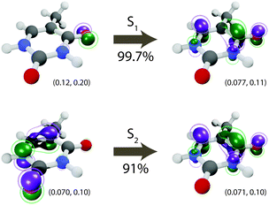 |
| | Fig. 1 Dominant natural transition orbitals (NTOs) for the S1 (n–π*) and S2 (π–π*) electronic states. The corresponding singular value is shown under the arrow. For each NTO, isovalues are shown below the corresponding orbital and chosen to contain approximately 25% (inner) and 50% (outer) of the total orbital density. All excitations at the Franck–Condon geometry. | |
Table 3 Computed vertical excitation energies for the first two singlet excited states of thymine compared to experimental results from gas-phase electron energy loss (EEL) spectroscopy (band maxima)
| Method |
S1 (eV) |
S2 (eV) |
| PBE0/SVP (this work) |
4.85 |
5.44 |
| PBE0/SVPD (this work) |
4.83 |
5.24 |
| ADC(2)52 |
4.56 |
5.06 |
| MS-CASPT250 |
5.09 |
5.09 |
| MS-CASPT243 |
5.23 |
5.44 |
| CASSCF50 |
5.31 |
7.12 |
|
|
| EEL spectroscopy |
|
4.95,89 4.9,90 4.9691 |
4.4 Dynamics
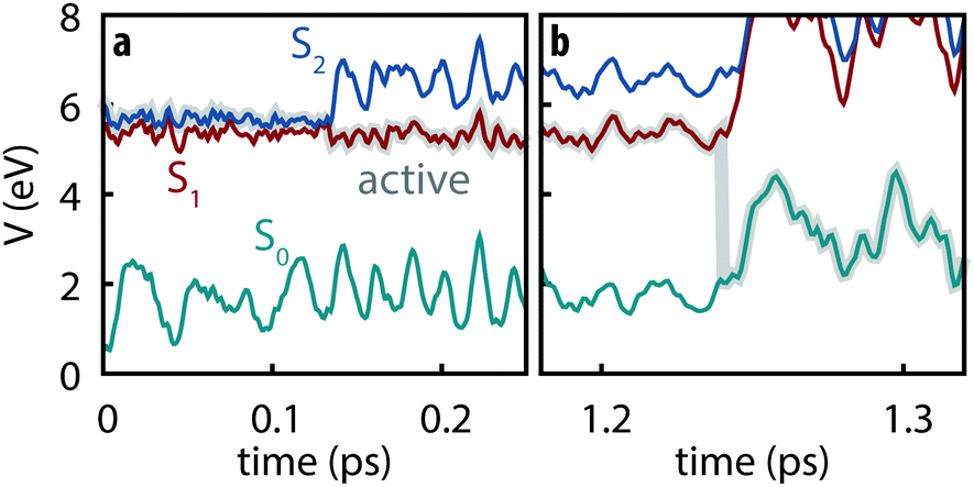
All simulated trajectories exhibit similar qualitative behavior exemplified by the sample trajectory shown in Fig. 2: after being initiated on the S2 state, thymine rapidly undergoes internal conversion to the S1 state (in all cases occurring in less than 250 fs) followed by a slower decay to S0 on the order of several ps.
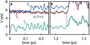 |
| | Fig. 2 Example trajectory showing (a) the subpicosecond internal conversion from S2 to S1 followed by (b) slow decay to S0. | |
Since the detailed nonadiabatic dynamics are expected to be highly sensitive to the energy difference between different excited states—which is itself sensitive to the basis set—we first assessed the difference between observed dynamics using both def2-SVP and def2-SVPD basis sets. 100 trajectories were simulated for each basis set using FSSH and trajectories were propagated for 5 ps using def2-SVP and 1.5 ps using def2-SVPD. Fig. 3 compares the evolution of the excited state populations along these trajectories. Excited state populations in Fig. 3 were computed as pk(t) = Nk(t)/Ntraj where Nk(t) is the number of trajectories with state k as active state at time t.
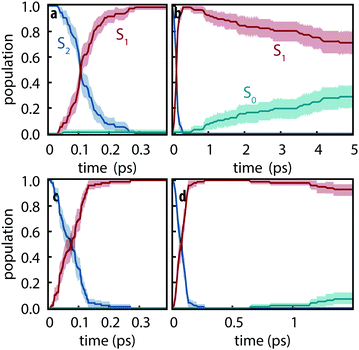 |
| | Fig. 3 Excited-state populations measured over trajectory swarms using (a and b) def2-SVP and (c and d) def2-SVPD basis sets. Shaded regions show the 95% bootstrap confidence interval. Panels (a) and (c) show the short time behavior while panels (b) and (d) show the picosecond behavior. Note the different time scales in (b) and (d). | |
The S2 decay with def2-SVPD was found to be significantly faster than with def2-SVP: with def2-SVP, the half-life of the S2 state is 106 fs (CI: 102–112 fs) whereas the half-life with def2-SVPD was 76 fs (CI: 57–89 fs). The observed increased rate can be attributed to the reduced energy gap at the Franck–Condon geometry between S1 and S2, ΔE21 = ES2 − ES1, which is 0.59 eV at def2-SVP and 0.41 eV at def2-SVPD, i.e., the energy gap and the half-life both reduce by ≈70%. On the other hand, since ΔE10 is only slighty affected by the basis set, no significant change in the S1 lifetime is expected or observed. After 1.5 ps, the proportion of trajectories on the ground state have strongly overlapping confidence interval ranges (6–18% with def2-SVP vs. 3–12% with def2-SVPD). We therefore conclude that after the ultrafast decay to S1, def2-SVP and def2-SVPD recover essentially identical dynamics and we thus continue our analysis with only the def2-SVP results.
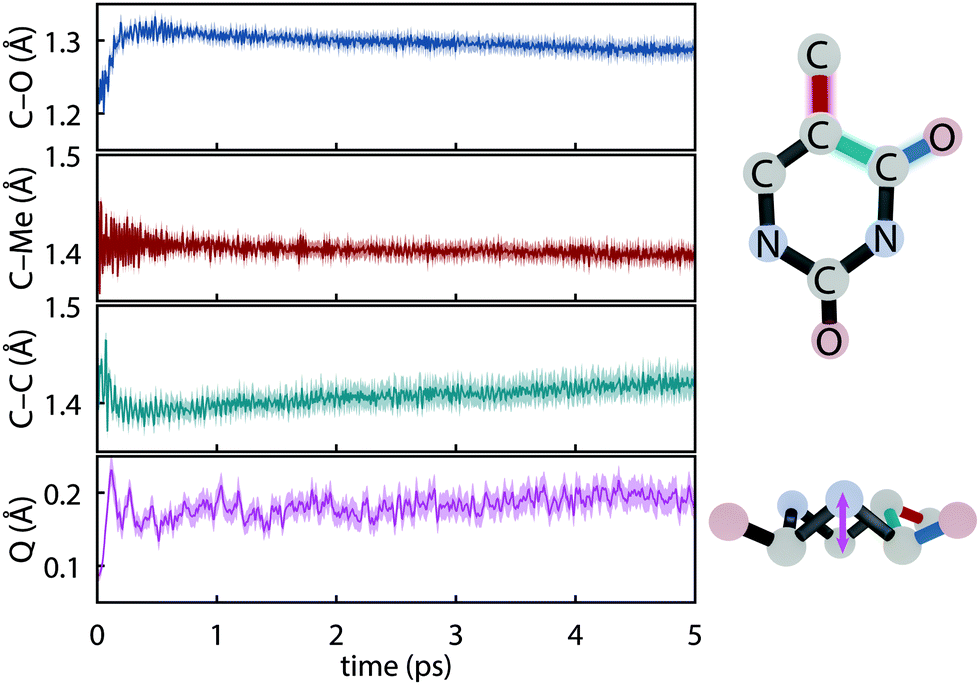
The initial dynamics were quantified in terms of four structural parameters, the C–O bond distance of the carbonyl on which the S1 hole is located, the C–Me (where Me is methyl), the C–C bond distance for the carbon atoms in the ring connecting the active carbonyl and the CMe, and the ring puckering amplitude, Q, computed using the Cremer–Pople coordinates.92Fig. 4 summarizes the dynamics simulated using FSSH and depicts the coordinates involved. Immediately upon photoexcitation, the C–O bond lengthens and the C–C bond shortens, both of which are consistent with observed shifts in the oxygen Auger spectrum44 and with the interpretation that the particle (virtual) NTO of the S2 excitation exhibits a bonding-like π overlap on the C–C bond in the ring and an antibonding-like structure on the carbonyl. In addition, the puckering amplitude more than doubles from the equilibrium value of about 0.08 Å to 0.23 Å within 120 fs. However, we find no significant difference in the degree of planarity between the ground state and S1, and thus attribute the increased degree of puckering to the increased vibrational energy resulting from the nonradiative decay.
 |
| | Fig. 4 Major geometrical changes measured over trajectory swarms accompanying ultrafast dynamics simulated with def2-SVP and FSSH. Shaded regions show the 95% bootstrap confidence interval. (a) C–O bond distance (b) C–Me bond distance (c) aromatic C–C bond distance and (d) the puckering amplitude, Q.92 | |
The simulated rates for the two electronic decays (S2 → S1 and S1 → S0) are characterized as single exponential decays from which two lifetimes are defined according to
and
| | | p0(t > 0) ≈ 1 − e−t/τ0, | (24b) |
where
τ2 corresponds to the S
2 → S
1 decay channel and
τ0 corresponds to the rise of the ground state or conversely the total excited state lifetime.
τ2 is estimated through the S
2 half-life,
tS2,1/2, according to
| | | τ2 = tS2,1/2/ln2, | (25) |
while
τ0 is similarly estimated from the final value in the simulation using
| | | τ0 = −tf/ln(1 − p0,f), | (26) |
where
tf and
p0,f =
p0(
tf) are the time and population used to estimate the rate.
Using the set of def2-SVP simulations, we find the S2 lifetime to be τ2 = 153 fs (CI: 147–162 fs) which agrees well with the 100–200 fs lifetimes measured for the prompt signal. Consequently, we assign the prompt signal to the S2 → S1 decay. The total excited state lifetime was found to be 13.9 ps (CI: 10.4–21 ps), which agrees well (within a factor of 2) with the 5–7 ps lifetimes measured for the fast component such that we assign the fast signal to correspond to the S1 → S0 decay.
4.5 Electronic populations and surface hopping
Electronic populations within FSSH and many of its variants are ambiguously defined93 because the FSSH algorithm refers to two distinct effective electronic wavefunctions: (i) the auxiliary wavefunction, which is propagated using eqn (2) and (ii) the active wavefunction which is determined from the evolution of the auxiliary wavefunction and from which the potential energy and nuclear forces are computed. The preceding analysis follows the original prescription8 in which only the active wavefunction (i.e. the active surface) is used to determine electronic populations although other prescriptions have been proposed.94 However, it is important to examine the auxiliary electronic populations because they indirectly dictate the behavior of the active wavefunction and because they are central to the original motivation for hopping probabilities.
Electronic populations using the auxiliary wavefunction indicate negligible nonradiative decay from S1; instead, the populations slowly evolve towards a near equal mixture of S1 and S2 (see Fig. 5). This leads to a starkly different interpretation of the reactivity—that S1 and S2 are equally populated on the picosecond timescale—that is not supported by any experimental evidence. This is concerning given that the FSSH hopping probabilty was derived to satisfy the constraint that the swarm-based populations, i.e., populations computed through
| | | pk(t) = 〈Nk〉(t)/Ntraj, | (27) |
where 〈
Nk〉(
t) is the number of trajectories with active surface
k at time
t and
Ntraj is the total number of trajectories, statistically match the auxiliary populations.
8 It thus appears that physically valid results for thymine are obtained even though a central assumption underlying surface hopping is violated. These results imply that efforts to adjust the surface hopping criterion to better enforce the correspondence between swarm-based populations and the auxiliary electronic density matrix could adversely affect accuracy for the present system.
95
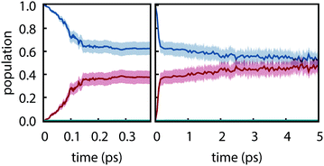 |
| | Fig. 5 Electronic populations computed from the auxiliary electronic density matrix for trajectories computed using PBE0-D3/def2-SVP and FSSH. Shaded regions show the 95% bootstrap confidence interval. (a) Short time and (b) long time behavior. | |
Our observation is consistent with previous work on multi-state FSSH96 and the fact that the total energy of a trajectory and all properties, including electronic populations, are best defined in terms of an energy derivative:97
| |  | (28) |
where
E(
t) is the trajectory energy which is defined as the nuclear kinetic energy plus the electronic energy of the active state.
5 Conclusions
Building on resource-efficient methodology previously developed for ground states, excited states, and quadratic response properties, the implementation of state-to-state derivative couplings reported here enables multistate nonadiabatic molecular dynamics simulations using hybrid-TDDFT for molecules with up to ∼100 atoms and ∼10 ps simulation times on single workstation nodes. For the first three singlet states of thymine, each step of an on-the-fly NAMD simulation including all couplings requires only a factor of 4.3 more CPU time than the corresponding ground-state AIMD simulation. As opposed to finite-difference approaches, the entire nonadiabatic coupling vector is obtained, enabling correct rescaling of velocities. The single Slater-determinant model for excited states corresponds to a zeroth-order noniterative approximation using unit excitation vectors and neglecting the Hartree, exchange, and correlation contributions to the excitation energy. Whether the resulting modest gain in efficiency is worthwhile in view of the loss of accuracy caused by neglect of configuration interaction appears questionable. Our implementation will be publicly released through Turbomole.98,99 All NAMD trajectory data are available through a Creative Commons license.100
Straightforward application of the present hybrid TDDFT-SH methodology to UV-photoexcited thymine semiquantitatively recovers experimental excited-state lifetimes. In particular, the TDDFT-SH lifetimes of 147–162 fs for S2 and 10.4–20.1 ps for S1 agree well with the experimentally observed ones of 100–200 fs and 5–7 ps. The rapid S2 decay is barrierless and proceeds through a conical intersection between S2 and S1 close to the Franck–Condon region, whereas the S1 decay is much slower. Thus, our results strongly support the S1 trapping hypothesis.43
For thymine deactivation, TDDFT using standard hybrid functionals yields significantly better agreement with experiment than MCSCF and ADC(2). While this result could be coincidential, it is consistent with the good performance of hybrid TDDFT for vertical excitation energies of thymine, as well as a mounting body of evidence suggesting that hybrid TDDFT has favorable cost-to-performance characteristics for a wide range of systems.13,16,20,25,26,101–108 Due to its resource efficiency, TDDFT-SH is particularly suitable for large-scale and exploratory applications. The striking discrepancy between electronic and trajectory-averaged populations for the slow decay of the S1 state of thymine may warrant further investigation. The current approach circumvents but does not fundamentally eliminate the divergences of inexact response theory in state-to-state properties.34,62
Conflicts of interest
Principal investigator Filipp Furche has an equity interest in Turbomole GmbH. The terms of this arrangement have been reviewed and approved by the University of California, Irvine, in accordance with its conflict of interest policies.
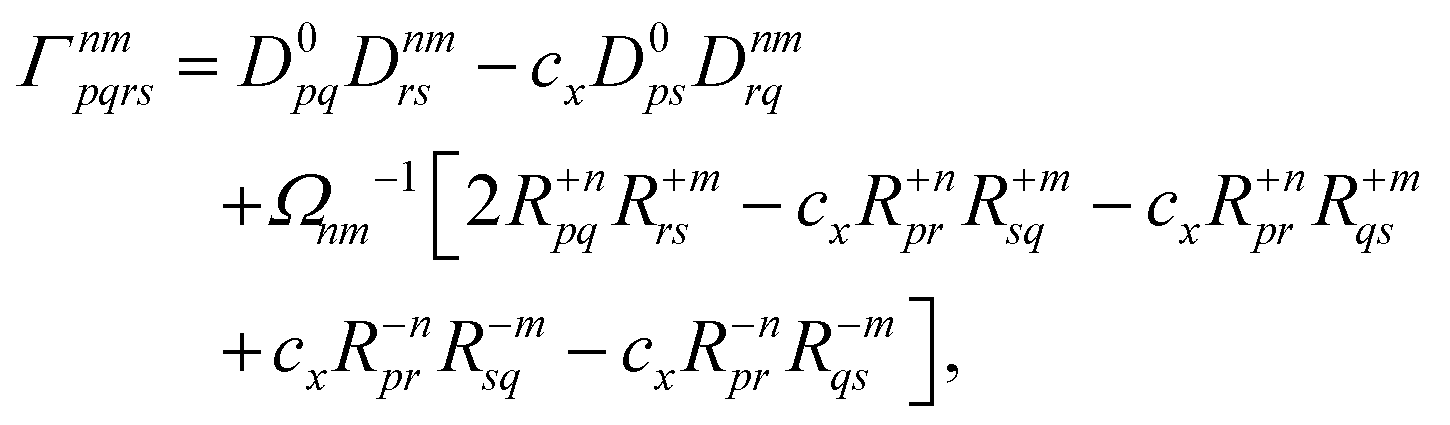
Appendix: derivation of state-to-state derivative coupling
We parametrize the state-to-state 1TDM in eqn (14) as| |  | (29) |
where Tnm is defined in eqn (17), and cQR is a constant that allows writing equations simultaneously for derivative couplings from quadratic response (cQR = 1) and pseudowavefunction (cQR = 0) approaches. For convenience, we define the linear transformations| |  | (30a) |
| |  | (30b) |
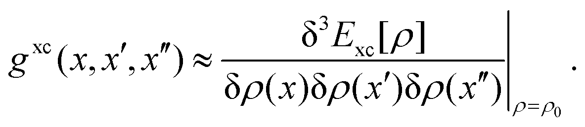
as well as the double contraction with the density functional hyperkernel,| | 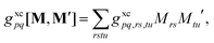 | (31) |
| |  | (32) |
In addition, we use the following shorthand definitions:| | 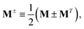 | (33b) |
| |  | (33d) |
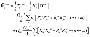
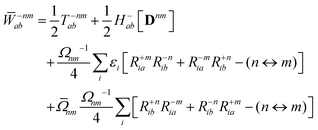
The orbital relaxation (off-diagonal) contributions to γnm require solution of
| | | |Xnm,Ynm〉 = −(Λ − ΩnmΔ)−1|Pnm,Qnm〉 | (34) |
with the right-hand-sides
| |  | (35a) |
| |  | (35b) |
where (
n ↔
m) signifies repeating the terms within the same bracket with
n and
m interchanged.
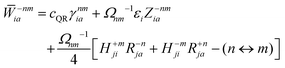
The Lagrange multiplier Dnm can be parametrized as
| | | Dnm = Ωnm−1(Tnm + Znm), | (36) |
where the diagonal blocks (
Ωnm−1Tnm) follow from
eqn (19) and
Znm is off-diagonal only. Next, expressions for
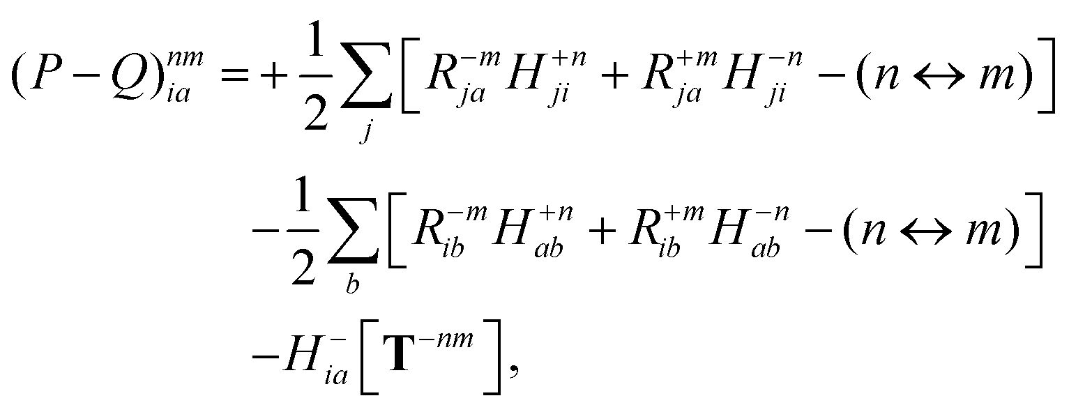
Znm are obtained by enforcing stationarity with respect to orbitals. We define
and
such that
| |  | (37a) |
| |  | (37b) |
| |  | (37c) |
| | | 〈Dnm,TC†FC〉(ap) = Dnmpaεp | (37d) |
| |  | (37e) |
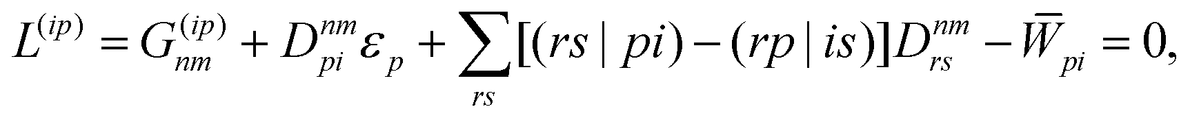
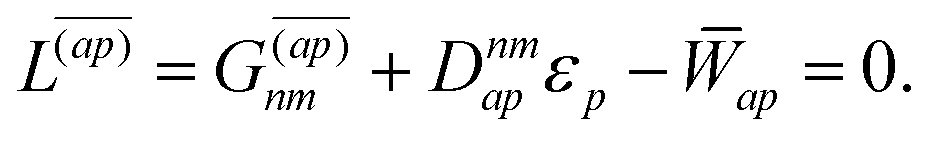
With this, the orbital stationarity conditions become
| |  | (38a) |
| |  | (38b) |
| | L(ap) = G(ap)nm + Dnmpaεp − ![[W with combining macron]](https://www.rsc.org/images/entities/i_char_0057_0304.gif) pa = 0, pa = 0, | (38c) |
| |  | (38d) |
Two sets of equations for the
Znm Lagrange multiplier are obtained by requiring

and

, which can be combined into
| | | Λ|Znm,ov,Znm,vo〉 − cQRΩnmΔ|Xnm,Ynm〉 = −|Pnm,Qnm〉. | (39) |
For derivative couplings based on quadratic response (
cQR = 1), this equation is satisfied by |
Zov,
Zvo〉 = |
Xnm,
Ynm〉 such that
while for derivative couplings based on the pseudowavefunction (
cQR = 0),
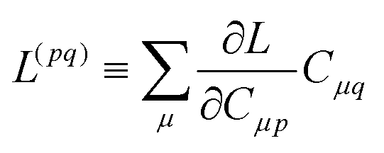
| | | |Znm,PW〉 = −Λ−1|Pnm,Qnm〉. | (41) |
The Lagrange multiplier nm is next determined from eqn (38) as
| |  | (42a) |
| |  | (42b) |
| |  | (42c) |
| |  | (42d) |
| |  | (42e) |
| |  | (42f) |
Finally, the pair-density in eqn (22) is
| |  | (43) |
where
R±n should be interpreted as an occupied–virtual-only matrix and
D(0)pq =
δpiδqi is the ground state density matrix.
Acknowledgements
This material is based upon work supported by the U.S. Department of Energy, Office of Basic Energy Sciences, under Award Number DE-SC0018352. S. M. P. is supported by an Arnold O. Beckman Postdoctoral Fellowship. The authors thank Alan Robledo for assistance.
Notes and references
- W. Domcke and D. R. Yarkony, Annu. Rev. Phys. Chem., 2012, 63, 325–352 CrossRef CAS PubMed.
- A. Zangwill and P. Soven, Phys. Rev. A: At., Mol., Opt. Phys., 1980, 21, 1561–1572 CrossRef CAS.
- E. Runge and E. K. U. Gross, Phys. Rev. Lett., 1984, 52, 997–1000 CrossRef CAS.
- M. Petersilka, U. J. Gossmann and E. K. U. Gross, Phys. Rev. Lett., 1996, 76, 1212–1215 CrossRef CAS PubMed.
-
E. K. U. Gross, J. F. Dobson and M. Petersilka, Density Functional Theory II, Springer-Verlag, Berlin/Heidelberg, 1996, pp. 81–172 Search PubMed.
- R. Baer, Chem. Phys. Lett., 2002, 364, 75–79 CrossRef CAS.
- R. Baer, Y. Kurzweil and L. S. Cederbaum, Isr. J. Chem., 2005, 45, 161–170 CrossRef CAS.
- J. C. Tully, J. Chem. Phys., 1990, 93, 1061 CrossRef CAS.
-
F. Agostini, B. F. E. Curchod, R. Vuilleumier, I. Tavernelli and E. K. U. Gross, in TDDFT and Quantum-Classical Dynamics: A Universal Tool Describing the Dynamics of Matter, ed. W. Andreoni and S. Yip, Springer International Publishing, Cham, 2018, pp. 1–47 Search PubMed.
- E. Tapavicza, G. D. Bellchambers, J. C. Vincent and F. Furche, Phys. Chem. Chem. Phys., 2013, 15, 18336–18348 RSC.
- C. F. Craig, W. R. Duncan and O. V. Prezhdo, Phys. Rev. Lett., 2005, 95, 163001 CrossRef PubMed.
- E. Tapavicza, I. Tavernelli, U. Rothlisberger, C. Filippi and M. E. Casida, J. Chem. Phys., 2008, 129, 124108 CrossRef PubMed.
- T. Thompson and E. Tapavicza, J. Chem. Phys., 2018, 9, 4758–4764 CAS.
- E. Tapavicza, A. M. Meyer and F. Furche, Phys. Chem. Chem. Phys., 2011, 13, 20986–20998 RSC.
- J. Kim, H. Tao, T. J. Martinez and P. Bucksbaum, J. Phys. B: At., Mol. Opt. Phys., 2015, 48, 164003 CrossRef.
- O. Schalk, T. Geng, T. Thompson, N. Baluyot, R. D. Thomas, E. Tapavicza and T. Hansson, J. Phys. Chem. A, 2016, 120, 2320–2329 CrossRef CAS PubMed.
- M. Barbatti, J. Pittner, M. Pederzoli, U. Werner, R. Mitrić, V. Bonačić-Koutecký and H. Lischka, Chem. Phys., 2010, 375, 26–34 CrossRef CAS.
- M. Sapunar, A. Ponzi, S. Chaiwongwattana, M. Malis, A. Prlj, P. Decleva and N. Doslic, Phys. Chem. Chem. Phys., 2015, 17, 19012–19020 RSC.
- M. Wohlgemuth, V. Bonačić-Koutecký and R. Mitrić, J. Chem. Phys., 2011, 135, 054105 CrossRef PubMed.
- L. Du and Z. Lan, J. Chem. Theory Comput., 2015, 11, 1360–1374 CrossRef CAS PubMed.
- A. V. Akimov, A. J. Neukirch and O. V. Prezhdo, Chem. Rev., 2013, 113, 4496–4565 CrossRef CAS PubMed.
- R. Long, J. Liu and O. V. Prezhdo, J. Am. Chem. Soc., 2016, 138, 3884–3890 CrossRef CAS PubMed.
- W. R. Duncan, W. M. Stier and O. V. Prezhdo, J. Am. Chem. Soc., 2005, 127, 7941–7951 CrossRef CAS PubMed.
- W. R. Duncan, C. F. Craig and O. V. Prezhdo, J. Am. Chem. Soc., 2007, 129, 8528–8543 CrossRef CAS PubMed.
- M. Muuronen, S. M. Parker, E. Berardo, A. Le, M. A. Zwijnenburg and F. Furche, Chem. Sci., 2017, 8, 2179–2183 RSC.
- J. C. Vincent, M. Muuronen, K. C. Pearce, L. N. Mohanam, E. Tapavicza and F. Furche, J. Phys. Chem. Lett., 2016, 7, 4185–4190 CrossRef CAS PubMed.
- Y. Han, B. Rasulev and D. S. Kilin, J. Phys. Chem. Lett., 2017, 8, 3185–3192 CrossRef CAS PubMed.
- E. Tapavicza, I. Tavernelli and U. Rothlisberger, Phys. Rev. Lett., 2007, 98, 023001 CrossRef PubMed.
- M. Wohlgemuth, V. Bonačić-Koutecký and R. Mitrić, J. Chem. Phys., 2010, 133, 194104 CrossRef PubMed.
- I. Tavernelli, B. F. E. Curchod and U. Rothlisberger, Chem. Phys., 2011, 391, 101–109 CrossRef CAS.
- B. Curchod, T. Penfold, U. Rothlisberger and I. Tavernelli, Cent. Eur. J. Phys., 2013, 11, 1059 CAS.
- T. Nelson, S. Fernandez-Alberti, V. Chernyak, A. E. Roitberg and S. Tretiak, J. Phys. Chem. B, 2011, 115, 5402–5414 CrossRef CAS PubMed.
- Z. Li, B. Suo and W. Liu, J. Chem. Phys., 2014, 141, 244105 CrossRef PubMed.
- Q. Ou, G. D. Bellchambers, F. Furche and J. E. Subotnik, J. Chem. Phys., 2015, 142, 064114 CrossRef PubMed.
- X. Zhang and J. M. Herbert, J. Chem. Phys., 2015, 142, 064109 CrossRef PubMed.
- S. M. Parker, D. Rappoport and F. Furche, J. Chem. Theory Comput., 2018, 14, 807–819 CrossRef CAS PubMed.
- H. Kang, K. T. Lee, B. Jung, Y. J. Ko and S. K. Kim, J. Am. Chem. Soc., 2002, 124, 12958–12959 CrossRef CAS PubMed.
- C. Canuel, M. Mons, F. Piuzzi, B. Tardivel, I. Dimicoli and M. Elhanine, J. Chem. Phys., 2005, 122, 074316 CrossRef PubMed.
- S. Ullrich, T. Schultz, M. Z. Zgierski and A. Stolow, Phys. Chem. Chem. Phys., 2004, 6, 2796 RSC.
- E. Samoylova, H. Lippert, S. Ullrich, I. V. Hertel, W. Radloff and T. Schultz, J. Am. Chem. Soc., 2005, 127, 1782–1786 CrossRef CAS PubMed.
- E. Samoylova, T. Schultz, I. V. Hertel and W. Radloff, Chem. Phys., 2008, 347, 376–382 CrossRef CAS.
- J. González-Vázquez, L. González, E. Samoylova and T. Schultz, Phys. Chem. Chem. Phys., 2009, 11, 3927 RSC.
- J. J. Szymczak, M. Barbatti, J. T. Soo Hoo, J. A. Adkins, T. L. Windus, D. Nachtigallová and H. Lischka, J. Phys. Chem. A, 2009, 113, 12686–12693 CrossRef CAS PubMed.
- B. K. McFarland, J. P. Farrell, S. Miyabe, F. Tarantelli, A. Aguilar, N. Berrah, C. Bostedt, J. D. Bozek, P. H. Bucksbaum, J. C. Castagna, R. N. Coffee, J. P. Cryan, L. Fang, R. Feifel, K. J. Gaffney, J. M. Glownia, T. J. Martinez, M. Mucke, B. Murphy, A. Natan, T. Osipov, V. S. Petrović, S. Schorb, T. Schultz, L. S. Spector, M. Swiggers, I. Tenney, S. Wang, J. L. White, W. White and M. Gühr, Nat. Commun., 2014, 5, 4235 CrossRef CAS PubMed.
- C. E. Crespo-Hernández, B. Cohen, P. M. Hare and B. Kohler, Chem. Rev., 2004, 104, 1977–2020 CrossRef PubMed.
- S. Perun, A. L. Sobolewski and W. Domcke, J. Phys. Chem. A, 2006, 110, 13238–13244 CrossRef CAS PubMed.
- G. Zechmann and M. Barbatti, J. Phys. Chem. A, 2008, 112, 8273–8279 CrossRef CAS PubMed.
- Z. Lan, E. Fabiano and W. Thiel, J. Phys. Chem. B, 2009, 113, 3548–3555 CrossRef CAS PubMed.
- M. Barbatti, A. J. A. Aquino, J. J. Szymczak, D. Nachtigallová, P. Hobza and H. Lischka, Proc. Natl. Acad. Sci. U. S. A., 2010, 107, 21453–21458 CrossRef CAS PubMed.
- D. Asturiol, B. Lasorne, G. A. Worth, M. A. Robb and L. Blancafort, Phys. Chem. Chem. Phys., 2010, 12, 4949 RSC.
- D. Picconi, V. Barone, A. Lami, F. Santoro and R. Improta, ChemPhysChem, 2011, 12, 1957–1968 CrossRef CAS PubMed.
- L. Stojanović, S. Bai, J. Nagesh, A. Izmaylov, R. Crespo-Otero, H. Lischka and M. Barbatti, Molecules, 2016, 21, 1603 CrossRef PubMed.
- R. Improta, F. Santoro and L. Blancafort, Chem. Rev., 2016, 116, 3540–3593 CrossRef CAS PubMed.
- J. C. Tully and R. K. Preston, J. Chem. Phys., 1971, 55, 562–572 CrossRef CAS.
- N. C. Blais and D. G. Truhlar, J. Chem. Phys., 1983, 79, 1334–1342 CrossRef CAS.
-
M. E. Casida, Time-Dependent Density Functional Response Theory for Molecules, in Recent advances in density functional methods, ed. D. P. Chong, World Scientific, Singapore, 1995, vol. 1, pp. 155–192 Search PubMed.
- F. Furche, J. Chem. Phys., 2001, 114, 5982–5992 CrossRef CAS.
-
E. Gross and W. Kohn, Advances in Quantum Chemistry, in Density Functional Theory of Many-Fermion Systems, ed. P.-O. Löwdin, Academic Press, 1990, vol. 21, pp. 255–291 Search PubMed.
- R. Send and F. Furche, J. Chem. Phys., 2010, 132, 044107 CrossRef PubMed.
- S. Fatehi, E. Alguire, Y. Shao and J. E. Subotnik, J. Chem. Phys., 2011, 135, 234105 CrossRef PubMed.
- X. Zhang and J. M. Herbert, J. Chem. Phys., 2014, 141, 064104 CrossRef PubMed.
- S. M. Parker, S. Roy and F. Furche, J. Chem. Phys., 2016, 145, 134105 CrossRef PubMed.
- F. Furche and R. Ahlrichs, J. Chem. Phys., 2002, 117, 7433–7447 CrossRef CAS.
- F. Furche, R. Ahlrichs, C. Wachsmann, E. Weber, A. Sobanski, F. Vögtle and S. Grimme, J. Am. Chem. Soc., 2000, 122, 1717–1724 CrossRef CAS.
- H. Weiss, R. Ahlrichs and M. Häser, J. Chem. Phys., 1993, 99, 1262–1270 CrossRef CAS.
- O. Treutler and R. Ahlrichs, J. Chem. Phys., 1995, 102, 346–354 CrossRef CAS.
- R. E. Stratmann, G. E. Scuseria and M. J. Frisch, J. Chem. Phys., 1998, 109, 8218–8224 CrossRef CAS.
- S. J. A. van Gisbergen, J. G. Snijders and E. J. Baerends, Comput. Phys. Commun., 1999, 118, 119–138 CrossRef CAS.
- A. Görling, H. H. Heinze, S. P. Ruzankin, M. Staufer and N. Rösch, J. Chem. Phys., 1999, 110, 2785–2799 CrossRef.
- F. Furche, B. T. Krull, B. D. Nguyen and J. Kwon, J. Chem. Phys., 2016, 144, 174105 Search PubMed.
- B. I. Dunlap, J. W. D. Connolly and J. R. Sabin, J. Chem. Phys., 1979, 71, 3396–3402 CrossRef CAS.
- S. Hirata and M. Head-Gordon, Chem. Phys. Lett., 1999, 314, 291–299 CrossRef CAS.
- S. Yarasi, S. Ng and G. R. Loppnow, J. Phys. Chem. B, 2009, 113, 14336–14342 CrossRef CAS PubMed.
- P. M. Hare, C. E. Crespo-Hernandez and B. Kohler, Proc. Natl. Acad. Sci. U. S. A., 2007, 104, 435–440 CrossRef CAS PubMed.
- D. Asturiol, B. Lasorne, M. A. Robb and L. Blancafort, J. Phys. Chem. A, 2009, 113, 10211–10218 CrossRef CAS PubMed.
- S. Yamazaki and T. Taketsugu, J. Phys. Chem. A, 2011, 116, 491–503 CrossRef PubMed.
- W. Weber and W. Thiel, Theor. Chem. Acc., 2000, 103, 495–506 Search PubMed.
- B. G. Levine, C. Ko, J. Quenneville and T. J. Martnez, Mol. Phys., 2006, 104, 1039–1051 CrossRef CAS.
- F. Plasser, R. Crespo-Otero, M. Pederzoli, J. Pittner, H. Lischka and M. Barbatti, J. Chem. Theory Comput., 2014, 10, 1395–1405 CrossRef CAS.
- S. Gozem, F. Melaccio, A. Valentini, M. Filatov, M. Huix-Rotllant, N. Ferré, L. M. Frutos, C. Angeli, A. I. Krylov, A. A. Granovsky, R. Lindh and M. Olivucci, J. Chem. Theory Comput., 2014, 10, 3074–3084 CrossRef CAS PubMed.
- J. Tao, J. P. Perdew, V. N. Staroverov and G. E. Scuseria, Phys. Rev. Lett., 2003, 91, 146401 CrossRef PubMed.
- S. Grimme, J. Antony, S. Ehrlich and H. Krieg, J. Chem. Phys., 2010, 132, 154104 CrossRef PubMed.
- S. Grimme, S. Ehrlich and L. Goerigk, J. Comput. Chem., 2011, 32, 1456–1465 CrossRef CAS PubMed.
- F. Weigend and R. Ahlrichs, Phys. Chem. Chem. Phys., 2005, 7, 3297–3305 RSC.
- C. Adamo and V. Barone, J. Chem. Phys., 1999, 110, 6158–6170 CrossRef CAS.
- D. Rappoport and F. Furche, J. Chem. Phys., 2010, 133, 134105 CrossRef PubMed.
- B. Efron, Ann. Stat., 1979, 7, 1–26 CrossRef.
- S. Nangia, A. W. Jasper, T. F. Miller and D. G. Truhlar, J. Chem. Phys., 2004, 120, 3586–3597 CrossRef CAS PubMed.
- R. Abouaf, J. Pommier and H. Dunet, Chem. Phys. Lett., 2003, 381, 486–494 CrossRef CAS.
- M. Michaud, M. Bazin and L. O. Sanche, Int. J. Radiat. Biol., 2011, 88, 15–21 CrossRef PubMed.
- I. V. Chernyshova, E. J. Kontros, P. P. Markush and O. B. Shpenik, Opt. Spectrosc., 2013, 115, 645–650 CrossRef CAS.
- D. Cremer and J. A. Pople, J. Am. Chem. Soc., 1975, 97, 1354–1358 CrossRef CAS.
- J. E. Subotnik, A. Jain, B. Landry, A. Petit, W. Ouyang and N. Bellonzi, Annu. Rev. Phys. Chem., 2016, 67, 387–417 CrossRef CAS.
- B. R. Landry, M. J. Falk and J. E. Subotnik, J. Chem. Phys., 2013, 139, 211101 CrossRef.
- L. Wang, D. Trivedi and O. V. Prezhdo, J. Chem. Theory Comput., 2014, 10, 3598–3605 CrossRef CAS PubMed.
- T. Nelson, S. Fernandez-Alberti, A. E. Roitberg and S. Tretiak, J. Chem. Phys., 2013, 138, 224111 CrossRef PubMed.
-
S. M. Parker and F. Furche, in Frontiers of Quantum Chemistry, ed. M. J. Wójcik, H. Nakatsuji, B. Kirtman and Y. Ozaki, Springer Singapore, Singapore, 2018, pp. 69–86 Search PubMed.
- F. Furche, R. Ahlrichs, C. Hättig, W. Klopper, M. Sierka and F. Weigend, Wiley Interdiscip. Rev.: Comput. Mol. Sci., 2013, 4, 91–100 Search PubMed.
- TURBOMOLE V7.4 2019, a development of University of Karlsruhe and Forschungszentrum Karlsruhe GmbH, 1989–2007, TURBOMOLE GmbH, since 2007; available from http://www.turbomole.com.
-
S. M. Parker, S. Roy and F. Furche, Multistate hybrid time-dependent density functional theory with surface hopping accurately captures ultrafast thymine photodeactivation, UC Irvine Dash, Dataset, 2019, https://doi.org/10.7280/D1Q08V.
- G. Pereira Rodrigues, E. Ventura, S. A. do Monte and M. Barbatti, J. Phys. Chem. A, 2014, 118, 12041–12049 CrossRef CAS PubMed.
- D. Tuna, N. Došlić, M. Mališ, A. L. Sobolewski and W. Domcke, J. Phys. Chem. B, 2015, 119, 2112–2124 CrossRef CAS PubMed.
- D. Fazzi, M. Barbatti and W. Thiel, J. Am. Chem. Soc., 2016, 138, 4502–4511 CrossRef CAS PubMed.
- A. Prlj, N. Došlić and C. Corminboeuf, Phys. Chem. Chem. Phys., 2016, 18, 11606–11609 RSC.
- B. Marchetti and T. N. V. Karsili, Phys. Chem. Chem. Phys., 2016, 18, 3644–3658 RSC.
- M. Mališ and N. Došlić, Molecules, 2017, 22, 493 CrossRef.
- C. Wiebeler, F. Plasser, G. J. Hedley, A. Ruseckas, I. D. W. Samuel and S. Schumacher, J. Phys. Chem. Lett., 2017, 8, 1086–1092 CrossRef CAS PubMed.
- C. Cisneros, T. Thompson, N. Baluyot, A. C. Smith and E. Tapavicza, Phys. Chem. Chem. Phys., 2017, 19, 5763–5777 RSC.
Footnote |
| † Present address: Department of Chemistry, Case Western Reserve University, 10900 Euclid Ave., Cleveland, OH 44106, USA. |
|
| This journal is © the Owner Societies 2019 |
Click here to see how this site uses Cookies. View our privacy policy here. 
 Open Access Article
 This Open Access Article is licensed under a
  *,
Saswata
Roy
*,
Saswata
Roy


 ,63 building on the existing implementation of excited-state gradients and ground-to-excited-state derivative couplings. The rate-determining steps are the computation of a user-specified set of excitations, eqn (7), the construction of the relaxed densities, eqn (16), and the final contraction of the effective densities with operator partial derivatives, eqn (22). First, a user-specified set of excited states are computed, then couplings are computed between all excitations in a user-specified subset of the original excitations. For each pair of excited states, one coupled-perturbed Kohn–Sham (CPKS) calculation is required (for derivative couplings within full quadratic response theory, this becomes a dynamic polarizability calculation). The right-hand-sides for all pairs of excited states in eqn (16) are computed simultaneously, together with the right-hand-sides for excited-state gradients,63 using identical methodology as excited-state absorption calculations.36 Thus the state-to-state derivative coupling implementation achieves the same high resource-efficiency as shown for other quadratic response properties,36 up to the final contraction with operator derivatives. The required CPKS calculations were performed iteratively and simultaneously as described in ref. 36 and 64 with an integral driven65–69 nonorthonormal Krylov space block Davidson algorithm.70 Finally, for each operator type (e.g., h), contractions between its partial derivatives (h(ξ)) and all effective densities—including effective densities needed to compute ground- and excited-state gradients—were performed together such that the partial derivatives only need to be computed once.
 ).
).
 ), and excited states were converged to a residual norm of less than 10−7 (
 ). As for ADC(2), conical intersections between the ground state and an excited state have incorrect dimensionality with TDDFT.78 To avoid potential associated instabilities, trajectories are forced to hop to the ground state if the first excitation energy, Ω1, falls below 0.5 eV. In total, we simulated 200 independent trajectories for a combined 650 ps of simulation time.


 and
and  such that


 and
and  , which can be combined into