
 Open Access Article
 This Open Access Article is licensed under a Creative Commons Attribution-Non Commercial 3.0 Unported Licence
Ionic liquids from a fragmented perspective†
Justin A.
Conrad
,
Shinae
Kim
and
Mark S.
Gordon
 *
*
Department of Chemistry, Iowa State University, Ames, IA 50014, USA. E-mail: mark@si.msg.chem.iastate.edu
First published on 20th July 2019
Abstract
The efficacy of using fragmentation methods, such as the effective fragment potential, the fragment molecular orbital and the effective fragment molecular orbital methods is discussed. The advantages and current limitations of these methods are considered, potential improvements are suggested, and a prognosis for the future is provided.
Justin Conrad was born in Texas, United States, in 1989. He received BS degrees in both Mathematics and Chemistry from the College of the Ozark's in 2011. He completed his PhD in Theoretical Chemistry from Iowa State University in 2018. He is currently a postdoctoral fellow at Ames laboratory on the Iowa State University campus. His research focuses on the use of quantum-based fragmentation methods in modeling chemical systems, including ionic liquids and deep eutectic solvents. |
Shinae Kim was born in Seoul, South Korea. She received BSc in both chemistry and chemical engineering from Purdue University in 2012. She completed her Master's degree under supervision of Prof. Nikita Matsunaga from Long Island University – Brooklyn in 2015. Currently she is pursuing her PhD under the guidance of Prof. Mark S. Gordon from Iowa State University. Her research is focused on chemical interactions in chemical systems using fragmentation-based methods such as Effective Fragment Potential (EFP) and Effective Fragment Molecular Orbital (EFMO) methods. |
Mark Gordon, Distinguished Professor of Chemistry at Iowa State University was born in New York City. He completed his BS in Chemistry at RPI and his PhD in 1967 with John Pople at Carnegie-Mellon. Following postdoctoral research with Klaus Ruedenberg at Iowa State, Gordon joined the faculty at North Dakota State University. He moved to ISU in 1992. Gordon's research interests are in electronic structure theory, the theory of liquids, surface science, the design of new materials, and chemical reaction mechanisms. He received the ACS Awards for Computers in Chemical and Pharmaceutical Research in 2009 and Theoretical Chemistry in 2015. |
Introduction
Ionic liquids (ILs) are an intriguing class of compounds. Belonging to a subset of molten ionic salts with melting points near or less than 100 °C, some ionic liquids have melting points below room temperature (room temperature ionic liquids, RTILs). There has been much excitement and promise in recent years over the possible applications of ILs, some of which have come to fruition.1 For example, there has been considerable success in using ILs in carbon dioxide capture processes with an expectation of refrigeration applications, as well as syntheses of energetic ionic liquids (EILs) as explosives and as rocket fuels.1–4Much thought has also been applied to the use of ILs as solvent-free electrolyte solutions, in which the solvent is the electrolyte.5,6 A desirable application of this approach is to replace highly volatile organic solvent based electrolyte solutions in dye sensitized solar cells with ILs.6,7
While specific properties can differ considerably among ILs, some important properties are their extremely low vapor pressures8,9 (negligible in some ILs) and customizability in synthesis by the simple choice of anion–cation pairing, or even mixtures of anions or cations, sometimes referred to as IL melts.1,6 Many organic precursors to common IL cations can also be easily altered by organic synthesis substitution methods as well, adding another layer of customizability.1
The chemistry and physics of ILs result from a balance between attractive and repulsive interactions among the ions. There is often large delocalization of charge within the ions, and large asymmetric and sterically hindered structures that make crystal lattices difficult to form.1,10 Protic ionic liquids have an added complexity regarding how much of the IL consists of ions or neutral molecules; that is, the degree of ionicity.11
With balanced intermolecular interactions, small changes in quantum-based effects (such as dispersion or charge transfer) can play important roles in IL properties.12,13 Therefore, ILs are challenging to model classically, with the more successful force fields accounting for polarization and partial charges; some force fields include varying charges.13,14 But even sophisticated classical force fields only provide accurate predictions of some properties of some ILs and not others.
Quantum based methods are necessary to model ILs accurately; however, traditional quantum methods that incorporate electron correlation (e.g., second order perturbation theory (MP2), coupled cluster (CC) theory) are too computationally expensive to model much more than small gas phase clusters of ions. The need to combine condensed phase simulations with the accuracy of fully quantum calculations leads to the main focus of this perspective: modeling ionic liquids with ab initio based fragmentation methods.15,16 Fragmentation methods divide the computation of large chemical systems into smaller, well-defined fragments that can be calculated independently with high accuracy. Subsequently, all of the individual fragment data is combined in such a way as to retain accuracy for the entire system.16 This perspective examines some of the ab initio based fragmentation methods that have been used to model ILs, their utility, their limitations, some misconceptions, and some discussion on developing future methods for ILs.
Effective fragment potential (EFP) method
The effective fragment potential (EFP) method is a non-empirical polarizable force field generated from first principle quantum mechanics calculations,17,18 and is available in the general atomic and molecular electronic structure software (GAMESS) package19,20 and the LIBEFP library.21,22 Originally designed as an explicit solvent model, EFPs can be generated for any closed shell chemical species as non-covalently bonded fragments. The internal geometry of an EFP fragment is held rigid. Therefore, the EFP interaction energy only accounts for intermolecular interactions, which are described by five types of potentials:| EEFP = ECoul + Epol + Eexrep + Edisp + ECT | (1) |
The terms in eqn (1) correspond to Coulomb, polarization, exchange-repulsion, dispersion and charge transfer, respectively.13,17
While the EFP method has been shown to successfully model interaction energies with essentially MP223 accuracy in molecular systems, the method has not been widely applied to modeling ILs.
A benchmark study by Tan and Izgorodina24 compared the EFP method to the symmetry adapted perturbation theory method SAPT2 + 3 for modeling interaction energies between various IL ion pairs over several geometric configurations, pairing eight different anions with eight different cations that are commonly found in IL compounds. The authors noted that there are up to 20% differences between the EFP and SAPT2 + 3 predicted interaction energies, with the charge transfer energy component having the largest percent differences. This difference in CT energy was particularly apparent for halide anions (chloride and bromide), with some CT energies reported as positive, that is repulsive, an indication that something is incorrect.
Nebgen et al.25 reported the use of EFPs to predict nanostructures in self-assembling ILs. In that study, EFP molecular dynamics (MD) simulations with varying concentrations of water were performed on ion pairs of three ILs (3-methyl-1-pentylimidazolium cation paired with either chloride, nitrate or thiocyanate). Each of the ILs have known and increasing levels of self-assembly (gelatinization) in water. Evaluating the short range structural ordering among cation, anion and water, the EFP MD radial distribution functions (RDFs) and preferred geometric configurations of the anions at the first and second solvation shells were compared to small-angle X-ray scattering, wide-angle X-ray scattering, and 1H NMR experimental results. The EFP-MD predictions are in good agreement with the experimental findings. For thiocyanate, the EFP-MD simulations were able to explain the absence of the interaction of the anion with the protons on the imidazolium ring inferred from the 1H NMR experiments.25
Due to the apparent disparity between the two aforementioned studies, it is interesting to examine more closely the efficacy of the EFP method for modeling ILs.
Consider the terms in eqn (1) in more detail. The Coulomb term Ecoul in eqn (1) is obtained using the Stone distributed multipolar analysis (DMA), expanded through octopoles with expansion points at the atom centers and bond midpoints.26,27
The polarization term (Epol) is represented by the interaction of the induced dipole on one fragment with the permanent dipole on another fragment, expressed in terms of the dipole polarizability. Although this is just the first term of the polarizability expansion, it is robust because the molecular polarizabilities are expressed as distributed tensor sums of localized molecular orbital (LMO) polarizability tensors on individual bonds and lone pairs. The LMO polarizability tensors are iterated in a self-consistent manner, thereby incorporating many body effects.
The dispersion interaction (Edisp) can be expressed as an inverse R expansion,
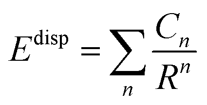 | (2) |
The exchange repulsion interaction (Eexrep) is derived as a power series expansion in the intermolecular overlap, truncated at the second order using LMOs.35 When the overlap expansion is expressed in terms of frozen LMOs on each fragment, the expansion can reliably be truncated at the quadratic term.35 The expression for Eexrep requires that each EFP carries a basis set.
The charge transfer interaction ECT is obtained using second-order perturbation theory.36 In the EFP method, charge transfer (CT) is defined as the interaction between the valence orbitals of one fragment and the virtual orbitals of another fragment.
There are several considerations that must be addressed regarding ECT especially when modeling charged species such as ILs. Of primary importance is a working definition of the virtual spaces of fragments. Currently there are two options for defining virtual spaces in the EFP method: the use of canonical molecular orbitals (CMO) that requires the full virtual space as determined by the basis set employed, and the valence virtual orbitals (VVO) that require only a subset of the virtual space, as defined by the occupied space.18,36,37 Since the full virtual space increases with the size of the basis set, the computational cost of the CMO option increases accordingly. In contrast, the size of the VVO virtual space is determined by the number of occupied valence orbitals and is therefore constant. The VVO option is the default in GAMESS, but care needs to be taken when using this option.
The VVOs are generated by projecting the CMOs onto an accurate atomic minimal basis set (AAMBS) via a singular value decomposition. The products of this projection are the quasi-atomic molecular basis orbitals (QUAMBOs), which can be further classified into three distinct orbital spaces: occupied core orbitals, occupied valence orbitals, and valence virtual orbitals (VVOs).37,38 The VVO space produced from this projection contains orbitals that resemble the atomic-like anti-bonding orbitals that complement the corresponding occupied orbitals.
By using VVOs, two issues could arise in the CT term for ions. First, it is not certain that the VVO approximation is an adequate approach for ionic fragments. Secondly, the VVO approximation is not appropriate for atomic fragments with noble gas electronic states (e.g. halides), since the VVO space would be null for atomic systems with noble gas electronic states (i.e. their s + p blocks are already full). Therefore, the CT energy for halide anions should be zero, as they would have no VVO space. So, the use of the VVO option for such species is not appropriate, and the CT energies for halide anions should use the full CMO virtual space. It should be noted that GAMESS clearly tells the user that there are no VVOs when the VVO approximation is used on a null space.
Another consideration for the CT energy is the basis set used for generating the orbitals. It was demonstrated in the first paper that introduced the general EFP method that the smallest basis set that should be used with this method is 6-31++G(d,p), in order to obtain consistently acceptable results.39 Furthermore, the 6-311++G(3df,2p) basis set40–42 is highly recommended for the greatest accuracy compared to SAPT results.43,44 This is especially important for CT energies produced using the CMO approximation, which is heavily basis set dependent. Finally, note that because effective fragment potentials are generated using Hartree–Fock (HF) and time-dependent HF calculations, the Pople basis sets are strongly recommended. It is well known that the correlation consistent basis sets used to generate the EFPs by Tan and Izgorodina24 are not reliable for HF calculations and should therefore not be used to generate EFPs.
Reevaluating the EFP energy terms with the recommended 6-311++G(3df,2p) basis set (except for bromide anion for which the G3Large basis was used) over the all ion pair configurations explored by Tan and Izgorodina,24 calculated with the CMO and VVO approximations, produces the results in Tables 1 and 2. The results in Table 1 demonstrate that the EFP method does have difficulty modeling charge transfer for halide anions, even with the appropriate CMO virtual space, but does better with the larger recommended Pople basis set, averaging to within 3 kcal mol−1 of SAPT2 + 3 charge transfer results. Excluding halides, on average the EFP method performs acceptably well modeling charge transfer energies, especially with the recommended basis set, approaching a near 1 kcal mol−1 difference from SAPT2 + 3 for the typical ionic liquid anions (TILA), as defined by Tan and Izagordina [TILA: tetrafluoroborate, dicyanamide, mesylate, bis{(trifluoromethyl)sulfonyl}amide, hexafluorophosphate, and tosylate], Fig. 1, even with the VVO virtual space. The lower standard deviation of the VVO CT energies may be attributed to the fact that the VVO approximation is nearly basis set independent because of a fixed virtual space, while the standard deviation CMO CT energies decreases as the basis set increases.
| Cations | Anions | ACCDa | ACCTa | 6-311++G(d,p) | 6-311++G(3df,2p) | |||||
|---|---|---|---|---|---|---|---|---|---|---|
| CMO | VVO | CMO | VVO | CMO | VVO | CMO | VVO | |||
| a SAPT2 + 3, EFP/ACCD and EFP/ACCT data taken from ref. 24. | ||||||||||
| Charge transfer | CnMIM | TILA | 1.2 ± 0.4 | 0.7 ± 0.4 | 1.5 ± 1.5 | 1.2 ± 0.3 | 1.7 ± 1.1 | 1.0 ± 0.5 | ||
| Hal | 9.7 ± 3.9 | 7.7 ± 5.1 | 4.4 ± 2.7 | 4.0 ± 3.7 | ||||||
| All | 4.1 ± 4.6 | 3.1 ± 4.4 | 2.5 ± 2.4 | 2.5 ± 2.5 | ||||||
| CnMPyr | TILA | 1.3 ± 0.5 | 0.5 ± 0.3 | 0.8 ± 0.7 | 1.1 ± 0.3 | 0.6 ± 0.4 | 1.0 ± 0.4 | |||
| Hal | 6.2 ± 0.8 | 3.4 ± 0.7 | 2.0 ± 1.6 | 1.7 ± 1.8 | ||||||
| All | 2.4 ± 2.1 | 1.2 ± 1.3 | 1.1 ± 1.1 | 0.9 ± 1.0 | ||||||
| All | TILA | 1.3 ± 0.5 | 0.6 ± 0.4 | 1.1 ± 1.1 | 1.1 ± 0.3 | 1.1 ± 1.0 | 1.0 ± 0.4 | |||
| Hal | 8.2 ± 3.5 | 5.8 ± 4.4 | 3.3 ± 2.5 | 3.0 ± 3.2 | ||||||
| All | 3.2 ± 3.6 | 2.1 ± 3.3 | 1.7 ± 1.9 | 1.6 ± 2.1 | ||||||
| Cations | Anions | ACCDa | ACCTa | 6-311++G(d,p) | 6-311++G(3df,2p) | |||||
|---|---|---|---|---|---|---|---|---|---|---|
| CMO | VVO | CMO | VVO | CMO | VVOb | CMO | VVOb | |||
| a SAPT2 + 3, EFP/ACCD and EFP/ACCT data taken from ref. 24. b SAPT2 + 3 and EFP of halide charge transfer energies were excluded from these total energies. | ||||||||||
| Total energy | CnMIM | TILA | 7.9 ± 6.5 | 6.9 ± 2.8 | 9.9 ± 18.9 | 8.2 ± 17.2 | 9.4 ± 17.6 | 7.7 ± 18.2 | ||
| TILA (no tos) | 6.4 ± 2.0 | 6.2 ± 2.1 | 3.0 ± 2.2 | 2.0 ± 1.6 | 3.5 ± 1.8 | 1.8 ± 1.3 | ||||
| Hal | 4.3 ± 2.7 | 6.0 ± 4.6 | 17.0 ± 5.4 | 12.9 ± 5.9 | 7.6 ± 3.4 | 8.4 ± 3.4 | ||||
| All | 6.7 ± 5.8 | 6.6 ± 3.5 | 12.3 ± 16.0 | 9.8 ± 14.6 | 8.8 ± 14.5 | 8.0 ± 14.9 | ||||
| All (no tos) | 5.6 ± 2.5 | 6.1 ± 3.2 | 8.1 ± 7.7 | 6.0 ± 6.4 | 5.0 ± 3.2 | 4.2 ± 4.0 | ||||
| CnMPyr | TILA | 3.4 ± 2.0 | 3.7 ± 1.7 | 4.4 ± 7.1 | 3.1 ± 6.4 | 1.6 ± 1.7 | 1.2 ± 1.2 | |||
| TILA (no tos) | 3.1 ± 1.5 | 3.4 ± 1.4 | 2.2 ± 1.2 | 1.1 ± 0.9 | 1.2 ± 1.0 | 1.0 ± 0.5 | ||||
| Hal | 2.9 ± 2.1 | 2.0 ± 1.6 | 8.6 ± 2.9 | 7.4 ± 4.6 | 6.1 ± 2.1 | 5.1 ± 1.6 | ||||
| All | 3.3 ± 2.0 | 3.3 ± 1.8 | 5.4 ± 6.6 | 4.1 ± 6.3 | 2.6 ± 2.6 | 2.1 ± 2.1 | ||||
| All (no tos) | 3.1 ± 1.7 | 3.1 ± 1.6 | 3.8 ± 3.3 | 2.7 ± 3.6 | 2.4 ± 2.5 | 2.0 ± 2.0 | ||||
| All | TILA | 5.3 ± 5.0 | 5.1 ± 2.7 | 6.8 ± 13.8 | 5.3 ± 12.5 | 5.0 ± 12.3 | 4.1 ± 12.4 | |||
| TILA (no tos) | 4.5 ± 2.4 | 4.6 ± 2.2 | 2.6 ± 1.7 | 1.5 ± 1.3 | 2.2 ± 1.8 | 1.3 ± 1.0 | ||||
| Hal | 3.7 ± 2.6 | 4.3 ± 4.1 | 13.3 ± 6.1 | 10.4 ± 6.0 | 6.9 ± 3.0 | 7.0 ± 3.2 | ||||
| All | 4.9 ± 4.5 | 4.9 ± 3.2 | 8.6 ± 12.4 | 6.8 ± 11.3 | 5.5 ± 10.6 | 4.9 ± 10.7 | ||||
| All (no tos) | 4.3 ± 2.4 | 4.5 ± 2.9 | 5.8 ± 6.2 | 4.2 ± 5.4 | 3.6 ± 3.1 | 3.1 ± 3.2 | ||||
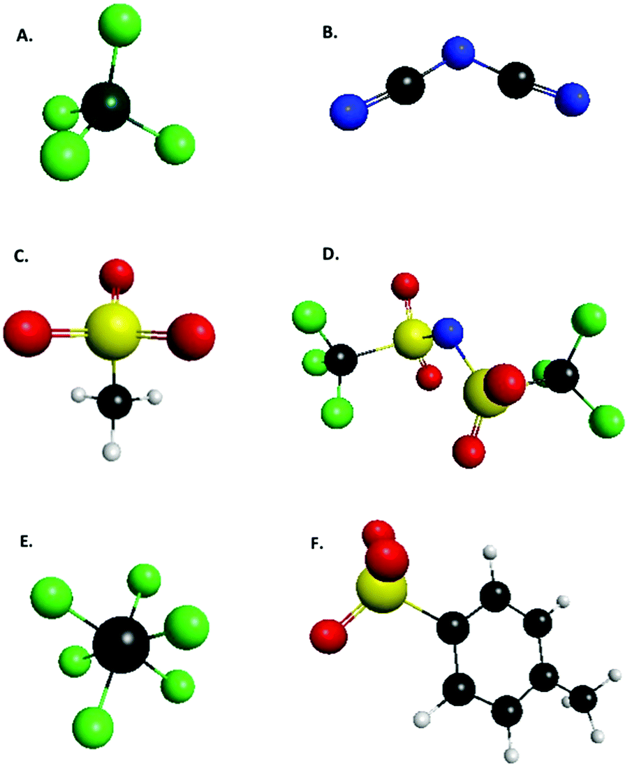 | ||
| Fig. 1 List of anions defined by Tan and Izagordina (ref. 24) as typical ionic liquid anions: (A) tetrafluoroborate, (B) dicyanamide, (C) mesylate, (D) bis{(trifluoromethyl)sulfonyl}amide, (E) hexafluorophosphate, (F) tosylate. | ||
Mean absolute differences of EFP total interaction energies are shown in Table 2. Note that the SAPT2 + 3 and EFP of halide CT energies are excluded from the total energies for the VVO approximation with the Pople basis sets. On average the EFP total interaction energies are within 5 kcal mol−1 of SAP2 + 3 results. This difference is further reduced to nearly within 1 kcal mol−1 for TILA, excluding tosylate and halide anions [TILA (no tos)], because it is difficult to charge transfer in systems with very localized charges as noted above. EFP greatly overestimates the tosylate electrostatic interaction in the tested ion pair configurations compared to SAPT2 + 3, particularly when the sulfonyl group directly interacts with the ring on the imdazolium cations, Fig. 2. This is believed to be due to (a) the ionic charge on tosylate being localized on the sulfonyl group rather than being delocalized across the entire anion and (b) the inability of a model potential like EFP to account for the actual transfer of electron density between fragments, which would be accounted for in fully quantum calculations. This overestimation of the electrostatic interaction of localized charge densities is also reflected in the total energies of the halide ion pairs. After re-evaluating these corrected benchmarks, it is clear that EFP can accurately model interaction energies for ions with large electronic delocalization [TILA (no tos)], and that the VVO approximation can be used effectively for these kinds of systems, when used appropriately (e.g., not halides).
 | ||
| Fig. 2 List of imidazolium and pyrrolidinium based cations used by Tan and Izagordina (ref. 24): (G) 1-methyl-3-methyl-imidazolium, (H) 1-methyl-3-ethyl-imidazolium, (I) 1-methyl-3-propyl-imidazolium, (J) 1-methyl-3-butyl-imidazolium, (K) N,N-dimethyl-pyrrolidinium, (L) N-ethyl-N′-methyl-pyrrolidinium, (M) N-propyl-N′-methyl-pyrrolidinium, (N) N-butyl-N′-methyl-pyrrolidinium. | ||
Another limitation of EFP, also noted by Nebgen et al.,25 is the internal rigidity of EFP fragments that in reality should have some torsional motions. Part of the success of Nebgen et al.25 in modeling ions as fragments can be attributed to their implementation of the recently reported mEFP (macromolecule EFP) method introduced by Slipchenko et al.,45 which allows the fragmentation of a macromolecule into smaller “bonded” EFP fragments. By using mEFP, some of the lost degrees of freedom can be reincorporated into the modeling of a macromolecule. Nebgen et al.25 modeled the imidazolium cation as two fragments: the long alkyl chain and the five-membered ring with the methyl group. The fragmentation was accomplished by neglecting interactions between bonded fragments and by using classical harmonic potentials for the covalent bonding during their MD simulations.
The effective fragment potential (EFP) method has the potential to be an effective tool in modeling ionic liquid (ILs), if used properly with an understanding of its underlying approximations and carefully determining which options will work for a desired system.
Embedding potential methods
The fragment molecular orbital (FMO) method, developed by Kitaura et al.,46 is an embedding method that is based on a many body expansion. Fragment based embedding methods calculate properties of the defined fragments individually within an embedding potential that approximates the environment (i.e., the rest of the system) surrounding each fragment.16 In the FMO method, each fragment energy is calculated at an ab initio level of theory (e.g., HF, MP2, CC) within the electrostatic potential (ESP) of the other fragments. The ESP is calculated via the one-electron Coulomb integrals using the electron densities of the other fragments. Since the energy of each monomer (single fragment) is dependent on the electron densities of all other fragments, the monomer energies are calculated iteratively until their energies stop changing to within a defined cut off. This FMO process is called the self-consistent charge (SCC) approach. If no explicit interactions between fragments are included, the method is called FMO1. The FMO energy can be further improved by calculating the explicit dimer energies (two-body energy terms across all fragment pairs). In this FMO2 method each dimer (fragment pair) is calculated at the chosen ab initio level embedded within the ESP of the other monomer densities. To avoid double counting, the energies of the two monomers within each dimer are subtracted out, as shown in eqn (3).16,46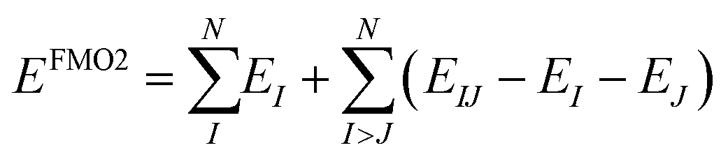 | (3) |
 | (4) |
Gao et al.48 reported the use of the explicit-polarization (X-pol)49 method to perform MD simulations of the IL 1-ethyl-3-methylimidazolium acetate. X-pol is an ab initio fragmentation method that is similar to FMO, in that it models a system as fragments within the embedding potential based on the densities of the other fragments. X-pol differs from FMO since the electrostatic interactions of the embedding potential are calculated from a multipole representation of densities of the other fragments, typically truncated at monopoles for efficiency.48,49
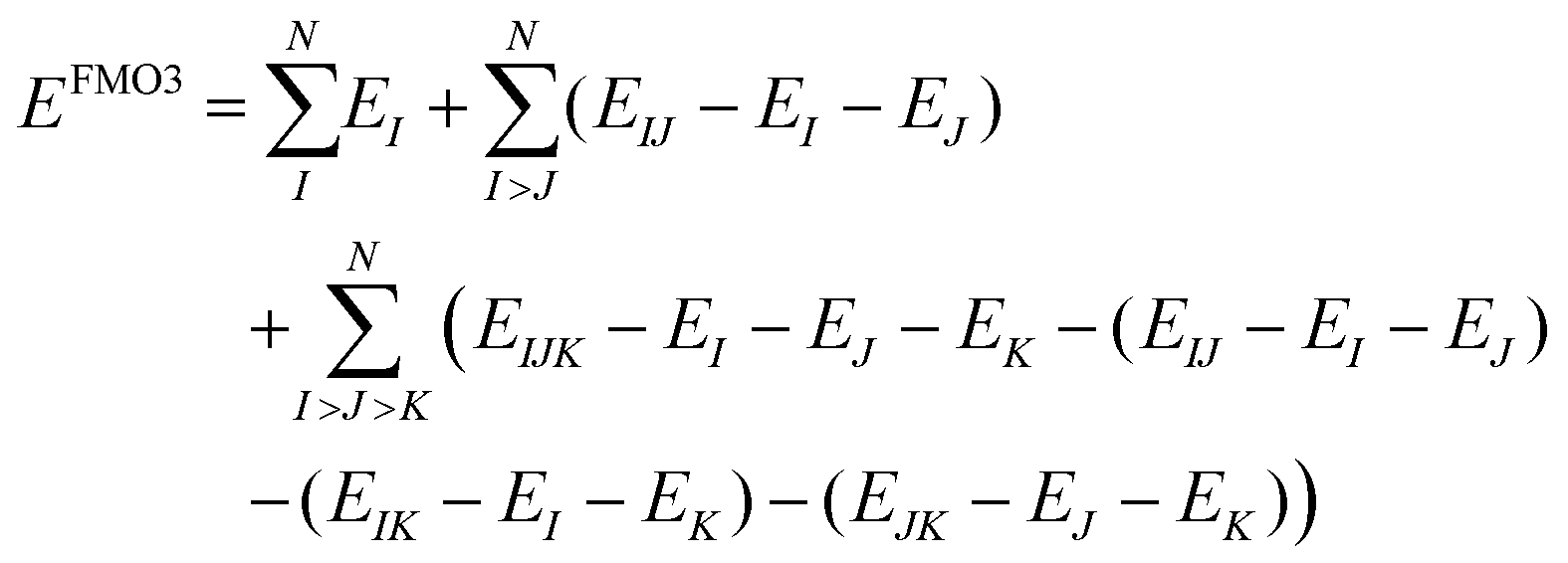
Several studies have already demonstrated the ability of FMO/MP2 to accurately represent MP2 for IL clusters, with FMO3 consistently achieving sub 1 kcal mol−1 accuracy. Carlson and co-workers50 reported sub kcal mol−1 recovery of the full MP2 relative energy for two ion pair structures of HEATN (1-hydroxyethyl-4-amino-1,2,4-triazolium nitrate) with both FMO2 and FMO3. Izgorodina et al. reported [ref. 51] sub kcal mol−1 recovery of the full MP2 energy for increasing cluster sizes of four ILs at both the FMO2 and FMO3 levels of theory. It was noted by the latter authors that the MP2 correlation energy correction increases rapidly with system size, thereby emphasizing the importance of using correlated QM methods to accurately predict IL properties.
To accurately model anions with quantum mechanical methods, it is necessary to include diffuse functions in the basis set to allow the electron density to expand and relax due to an increase in electron repulsion effects. In the FMO method, an increase in the electronic overlap of adjacent fragments due to the addition of diffuse functions can cause the SCC process to converge slowly, increasing the overall computational cost, or even prevent the SCC from converging at all. This leads to the question of how to accurately model ionic liquids with diffuse functions using FMO.
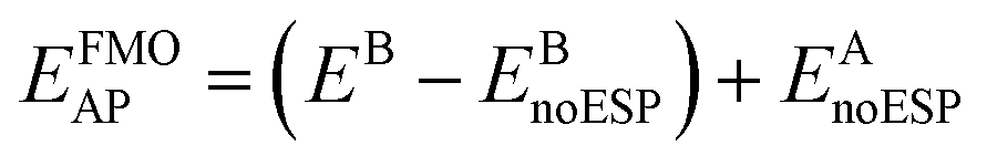
Several approaches have been utilized to solve this problem. The simplest, but not recommended, approach has been to disregard the use of diffuse functions for FMO calculations, accepting less accuracy to maintain efficiency. A second solution is to include diffuse functions for anion fragments only. This solution works reasonably well, so long as the nearest neighbors to a particular anion are not other anions. FMO-MD test simulations using this method perform better than simulations that use a single basis set with diffuse functions for all fragments. However, if two anion fragments come in close proximity to each other the SCC takes longer to converge, or becomes non-convergent. A third solution was developed by Fedorov and Kitaura.52 Termed auxiliary polarization (AP), this method employs the use of an auxiliary basis set to calculate the effective embedding potential, thereby avoiding the use of diffuse functions entirely in the SCC part of the calculation, while still being able to use diffuse functions in the quantum n-mer calculations.
The design of the AP basis set is a three-step procedure using a primary basis set (A) that would include diffuse functions for anions and an auxiliary basis set (B) that omits diffuse functions. First, the gas phase n-mers are calculated with the auxiliary basis, B, followed by a full FMO calculation again using auxiliary basis B. Subtracting the energy of the gas phase n-mers from the full FMO calculation results in the effective energy of the embedding potential using basis B. The third step is to calculate the energy of the gas phase n-mers with the primary basis, A, plus the previously calculated embedding potential energy, effectively calculating the ESP with auxiliary basis B. This may be expressed mathematically as
 | (5) |
The FMO method has the ability to break large covalent structures into separately defined fragments, without the use of capping.53 The procedure has its origins in the concept of localized charge distributions (LCD) originally developed by England and Gordon54 for semi-empirical methods and later by Jensen and Gordon for ab initio methods,55 in which two protons are “assigned” to each two-electron localized molecular orbital (LMO) to create a net neutral LCD. In the FMO method protons are likewise assigned to “move” with electrons to form what are called bond attached atoms and bond detached atoms. Like most fragmentation methods, the FMO method, and its more recent cousin, the effective fragment molecular orbital (EFMO) method56 cannot reliably fragment delocalized molecules, such as hexatriene or benzene.
In an effort to reduce the cost of modeling ILs with the FMO method, the covalent fragmentation method was explored using imidazolium cations as a test case, using FMO2 with dispersion-corrected HF, HF-D3. The 2-Frag model defines each ion as a fragment. The 3-Frag model defines the imidazolium ring and an attached alkyl chain split as two fragments, with the ring fragment having a net charge of +1 and the alkyl chain having zero net charge, and the anion being the third fragment, Fig. 3. The improved scaling of an eight ion pair cluster of 1-buyl-3-methylimidizolium [BMIM] hexafluorophosphate [PF6] can be seen in the dotted curves in Fig. 4. However, this improved scaling comes at a cost in accuracy, as the total interaction energy of the cluster is too low by ∼30 kcal mol−1. Electrostatic potentials reveal that the atomic charges on the ring change significantly (up to 0.5 e−) when the alkyl chain is separated from the ring. So, care must be taken when designing fragmentation schemes.
 | ||
| Fig. 3 FMO fragmentation schemes of 1-buyl-3-methylimidizolium cation for modeling 1-buyl-3-methylimidizolium hexafluorophosphate, with hexafluorophosphate anions defined as fragments in both schemes. Carbon and Nitrogen atoms are labeled. Hydrogen atoms are depicted in white. Scheme Frag-2 defines the entire cation as one fragment. Scheme Frag-3 divides the cation into two fragments, the 3-methylimidazolium ring which has the bond-attached nitrogen atom (NBAA) capped with a proton donated from the bond-detached boron atom (BBDA) of the butyl group and the butyl group with a frozen sp3 hybridized carbon molecular orbital on BBDA oriented over the detached bond. The proton donation allows closed shell fragments to break bonds heterolytically and remain closed shell. | ||
 | ||
| Fig. 4 Wall time per time step for two fragmentation schemes of 1-butyl-3-methylimidazolium hexafluorophosphate with FMO2-MD/RHF-D3 with the 6-31G(d) basis or with the 6-31G(d)/6-31+G(d) mixed basis that has diffuse functions on the anions. Simulations were over eight ion pairs. The 2-Frag scheme defines each ion as a fragment. The 3-Frag scheme defines each anion as one fragment and each cation as two fragments, with the butyl group taken to be a separate fragment. | ||
To determine how an alkyl chain can be fragmented without significantly changing the electron density on an imidazolium ring, 1-dodecyl-3methylimidixolium (C12MIM) cation was fragmented at each carbon along the 12-carbon chain. The atomic charges were then evaluated using electrostatic potential calculations. Atomic charges on the imidazolium ring are within 0.1 e− of their original charges when the alkyl chain is fragmented at the fourth carbon from the ring or further.
Another question regarding the use of the FMO method to model ILs is, at what inter-fragment distance(s) do dimer or trimer energy contributions become small enough that they can be excluded from the calculation to gain efficiency without significant loss in accuracy. This is an important question in developing cost efficient algorithms for MD simulations with periodic boundary conditions to model condensed phase IL phenomena. This question was partially explored by Halat and co-workers,57 on IL clusters of 4, 8, 16, and 32 ion pairs for eight ILs. They explored effective distance cut-offs for four components of the FMO energy: 2-body self-consistent field (SCF), 3-body SCF, 2-body electron correlation, and 3-body electron correlation. The SCF energies were calculated with HF and the electron correlation energy with MP2. While the preferred distance cutoffs varied depending on the specific IL, Halat and co-workers found on average that the SCF 2-body energy contributions are significant at all tested distances (tested up to 20 Å), while the 3-body SCF contributions are only significant when the three fragments are within 6 Å of each other. Electron correlation energies are well known to be short range, so it is not surprising that these authors concluded that the two-body (dimer) MP2 contributions to the energy are significant within 8 Å, while the 3-body (trimer) MP2 contributions to the energy are important only if the three fragments are within 4 Å of each other. Implementation of theses cutoffs for the 32 ion pair clusters effectively reduce the number of 3-body SCF calculations by 94%, 2-body MP2 calculations by 28%, and 3-body MP2 calculations by 89%. These are important findings for future FMO MD simulations of ILs.
The FMO method can take advantage of multilevel parallelism via the use of the general distributed data interface (GDDI).58 The GDDI approach facilitates coarse grain parallelism across compute nodes by computing each fragment on a different node or set of nodes. If the chosen electronic structure method (e.g., HF, MP2) has been implemented with a parallel algorithm, fine grain parallelism can be used within each node. It has been demonstrated that by taking advantage of the GDDI ansatz and eliminating I/O from the algorithm, FMO calculations scale nearly linearly to 262![[thin space (1/6-em)]](https://www.rsc.org/images/entities/char_2009.gif) 000 computer cores of a BlueGene/Q (BGQ) computer at Argonne National Laboratory.59,60 This capability was noted in a previous perspective.15
000 computer cores of a BlueGene/Q (BGQ) computer at Argonne National Laboratory.59,60 This capability was noted in a previous perspective.15
FMO molecular dynamics (MD) ionic liquid simulations were performed, using the BGQ, on four RTILs with clusters ranging from 8 ion pairs (IPs) to 16 IPs to 32 IPs. Several advantages and disadvantages of performing FMO/GDDI calculations on the BGQ were discovered. The main advantage is that the FMO/GDDI approach can fully utilize all 786432 cores across 48 racks. The main disadvantages are the limited I/O throughput and the limited memory per core. The I/O limitation has recently been eliminated as noted above. The memory limitation impacted the FMO/MP2 MD calculations for larger fragments; that is, for ILs with large cations. For those species, the calculations were performed using the FMO2/AP approach at the RHF-D3 level of theory. The main and auxiliary basis sets used were 6-31+G(d,p) and 6-31G, respectively. The MD simulations using this approach required ∼2–5 minutes of wall time per time step for an 8 IP system. This is, of course, much faster than what one could achieve with fully ab initio MD simulations (AIMD), and much slower than highly parameterized classical MD simulations.
These calculations revealed improvements that are needed for modeling ILs with fragmentation methods on two fronts. One is to develop improved software to simulate condensed phase phenomena using accurate quantum chemistry methods. Another is to develop more efficient models that retain the quantum effects that are important to correctly predict the dynamic properties of ILs. An important advance with regard to the latter is the recent development of analytic gradients for FMO using the resolution of the identity (RI) MP2 method. The FMO/RI-MP2 analytic gradient method will be available in GAMESS in the near future.
Moving toward condensed phase IL simulations
Periodic boundary conditions
In order for the FMO method to accurately model condensed phase IL systems and to accurately predict condensed phase properties, it is important to implement efficient codes for periodic boundary conditions (PBC). The existing FMO PBS code does not take advantage of the multilevel parallelism afforded by GDDI. An implementation of FMO2/PBC by Fujita, Nakano and Tanaka,61 implemented in the ABINIT-MPX program package, surrounds a unit cell by a number of “shells” of periodic image cells to effectively enlarge the embedding potential around the central cell. Their method also allows monomers from image cells to be included in dimer calculations, but it was implemented without fully analytic gradients, thereby hindering the achievement of energy conservation. This was demonstrated by Brorsen et al.,62 who developed the fully analytic FMO gradients and then implemented FMO2/PBC with good energy conservation.62 However, the PBC implementation by the latter authors does not account for the long-range electrostatic dimer approximation.47 The same is true for the more recent FMO3 implementation.60 This greatly reduces the computational efficiency of the method, since all dimers must be treated explicitly with the chosen electronic structure method when PBC are used. Therefore, to improve the efficiency and scalability of FMO/PBC simulations, the analytic gradient must include the long-range electrostatic term.Infinite coulomb potential
Though not trivial for ab initio methods, the development of a long-range Coulomb approximation for an infinite system (e.g. Ewald sums, or fast multipoles)63,64 are necessary for FMO PBC simulations to accurately model condensed phase IL systems.Periodic cell shape
Another potential improvement in efficiency might be provided by implementing a different shape for the periodic cell; for example, a truncated octahedron (TO)65 rather than a rectangular prism or a cube. The TO periodic cell is not commonly used in classical MD simulations due to the cost ratio (image cell algorithm complexity) vs. number of energy calculations. The TO requires fewer energy calculations but has a more complex and less vectorizable algorithm. In classical mechanics, energy calculations are typically very inexpensive, so the efficiency of the PBC has priority. However, for ab initio, including FMO, simulations the energy and gradient evaluations are much more computationally demanding, so the TO structure is an appealing alternative. Implementing a TO periodic cell would reduce the number of image cells from 26 to 14, reducing the required number of energy and gradient calculations. While a truncated octahedron is not efficient for modeling elongated, rigid systems (e.g. carbon nanotubes), it might be reasonable for modeling liquid dynamics for compounds like ILs that can naturally form a droplet shape.Improving computational efficiency
The use of MP2 with FMO MD simulations is desirable, because MP2 incorporates most of the essential physics required to provide accurate predictions. However, because MP2 calculations scale ∼N5 and have a significant memory demand, performing FMO/MP2 MD simulations is at present too computationally costly. A viable alternative would be to use the RI-MP2 approximation. RI-MP2 energies and gradients have recently been implemented in GAMESS,66 so FMO/RI-MP2 MD simulations are now a viable alternative.Currently, as noted above, the FMO method uses the electrostatic potential to describe long-range interactions. An alternative, and more accurate alternative treatment of long-range interactions is to use EFPs, since the EFP method captures intermolecular interactions with an accuracy that is comparable to that of MP2.67 This is accomplished by the effective fragment molecular orbital (EFMO) method, in which fragment–fragment (dimer) interactions are calculated using EFP interaction energies when the two fragments are separated by a distance that is longer than a user-defined cutoff distance Rcut. An additional advantage of the EFMO approach is that the EFP induction interaction captures the most important many-body effects since this term is iterated to self-consistency. This reduces the need for the much more computationally demanding FMO3 method for species (e.g., water) in which many body effects can be important. The EFMO method also removes the EFP constraint of rigid internal geometries. While this comes at the cost of having to generate EFPs at every time step in an MD simulation or geometry optimization, it comes at a more consistent and predicable cost than the SCC in the FMO method. For ILs, this also means not having to use a separate basis set for the ESP, as the SCC is avoided entirely. The short-range interactions that can be difficult for ion pairs treated by EFPs are avoided in EFMO, as short-range interactions are captured in the fully ab initio n-mer calculations.
Concluding remarks
The EFP method discussed in this work is based on accurate ab initio electronic structure methods with no empirically fitted parameters. This provides the EFP method with an important advantage over classical force fields that rely on fitted parameters and are therefore less extensible and less broadly applicable without extensive re-parameterization. The EFP method in addition has an accuracy for intermolecular interactions that is comparable to that of correlated electronic structure methods, such as second order perturbation theory (MP2).The FMO method scales linearly with system size, making this method applicable to very large systems. Because the FMO method can be combined with any electronic structure method, ranging from Hartree–Fock to density functional theory to correlated methods like MP2. So, the FMO method combines the accuracy and extensibility of correlated electronic structure theory with a scalability that facilitates its applicability to molecular dynamics and Monte Carlo simulations.
As noted above, effective fragment potentials (EFPs) can be a useful tool for modeling ILs, when utilized appropriately. The EFP method is capable of achieving at least MP2 accuracy for the prediction of intermolecular interactions. However, the charge transfer term is particularly sensitive to the choice of basis set. The recommended 6-311++G(3df,2p) basis set provides more accurate predictions of charge transfer interactions for EFPs. In addition, the valence virtual orbital (VVO) approximation for the EFP charge transfer interaction energy is inappropriate for halide anions, as the VVO space for atoms with noble gas atoms is null. For these cases, the canonical molecular orbital (CMO) virtual space should be used. The implementation of the new macromolecule EFP (mEFP) can improve dynamic simulations of larger ions by incorporating some of the internal degrees of freedom.25
The fragment molecular orbital (FMO) method has the ability to obtain great accuracy in modeling ILs, since the method is able to capture correlation energy interactions that classical methods have difficulty incorporating. The FMO method is much less computationally demanding than fully ab initio methods, because it can take advantage of multi-level parallelism and therefore scales nearly linearly. Nonetheless, the FMO method still requires some improvements to be able to efficiently perform condensed phase dynamic simulations of ILs, and to reach the time scales required to predict many dynamic properties, such as diffusion constants and ionicity. Implementing FMO periodic boundary conditions with a long-range Coulomb term (e.g., Ewald sums, fast multipoles) that fully utilize the multilevel parallelism of the FMO method will facilitate accurate modeling of condensed phase ILs. Utilizing the efficiency of the EFP method as an embedding potential for FMO (EFMO) enables the capture of short range many body correlation effects, increasing both the accuracy and the efficiency of the FMO method. Integration of the RI approximation to MP2 in FMO will further lower the computational cost for accurate IL simulations.
In addition to the aforementioned developments that will bring ab initio capability of treating condensed phase ionic liquids closer to reality, it is still desirable to develop accurate classical force fields that are amenable to much longer MD simulations and are therefore capable of predicting properties that require long timescales. One appealing approach for the development of accurate force fields is to capture the essential features of ab initio potentials by running FMO or EFMO MD simulations for shorter times and then using these potentials to develop new force fields. The use of ab initio potentials to generate new force fields is not a new idea,68 but the use of potentials based on fragmentation methods such as FMO and EFMO will make the process more efficient and effective.
The accurate modeling of ionic liquids is a challenging task. Ab initio based fragmentation methods are playing an increasingly important role in bridging the gap between the accuracy of fully ab initio calculations and the efficiency of classical dynamics models in order to accurately model and predict IL properties.
Conflicts of interest
There are no conflicts to declare.Acknowledgements
This work was supported in part by a grant from the U.S. Air Force Office of Scientific Research, Award No. FA9550-14-1-0306, and in part by a National Science Foundation Software Infrastructure grant, ACI-1047772. The authors are very grateful for many important and insightful discussions with Alex Findlater.References
- D. R. MacFarlane, N. Tachiwawa, M. Forsyth, J. M. Pringle, P. C. Howlett, G. D. Elliott, J. H. Davis Jr., M. Watanabe, P. Simon and C. A. Angell, Energy Environ. Sci., 2014, 7, 232 RSC.
- S. Zeng, X. Zeng, L. Bai, X. Zhang, H. Wang, J. Wang, D. Bao, M. Li, X. Liu and S. Zhang, Chem. Rev., 2017, 117(14), 9625–9673 CrossRef CAS PubMed.
- Q. Zhang and J. M. Shreeve, Chem. Rev., 2014, 114(20), 10527–10574 CrossRef CAS PubMed.
- G. Drake, T. Hawkins, A. Brand, L. Hall, M. McKay, A. Vij and I. Ismail, Propellants, Explos., Pyrotech., 2003, 28, 174 CrossRef CAS.
- D. Kuang, P. Wang, S. Itom, S. M. Zakeeruddin and M. Grätzel, J. Am. Chem. Soc., 2006, 128(24), 7732–7733 CrossRef CAS PubMed.
- X. Huang, D. Q. X. Zhang, Y. Luo, S. Huang, D. Li and Q. Meng, RSC Adv., 2013, 3, 6922–6929 RSC.
- Y. Lin., C. Li, C. Lee, Y. Leu, Y. Ezhumalai, Y. Ezhumalai, R. Vittal, M. Chen., J. Lin and K. Ho, ACS Appl. Mater. Interfaces, 2016, 8(24), 15267–15278 CrossRef CAS PubMed.
- J. M. S. S. Esperanca, J. N. C. Lopes, M. Tariq, L. M. N. B. F. Santos., J. W. Magee and L. P. N. Rebelo, J. Chem. Eng. Data, 2010, 55(1), 3–12 CrossRef CAS.
- M. A. A. Rocha, C. F. R. A. C. Lima, L. R. Gomes, B. Schröder, J. A. P. Coutinho, I. M. Marrucho, J. M. S. S. Esperançai, L. P. N. Rebelol, K. Shimizu, J. N. C. Lopesi and L. M. N. B. F. Santos, J. Phys. Chem. B, 2011, 115(37), 10919–10926 CrossRef CAS PubMed.
- M. Klähn, C. Stüber, A. Seduraman and P. Wu, J. Phys. Chem. B, 2010, 114, 2856 CrossRef.
- A. S. Amarasekara, Chem. Rev., 2016, 116(10), 6133–6183 CrossRef CAS PubMed.
- E. I. Izgorodina, D. Golze, R. Maganti, V. Armel, M. Taige, T. J. S. Schubert and D. R. MacFarlane, Phys. Chem. Chem. Phys., 2014, 16, 7209–7221 RSC.
- K. Dong, X. Liu, H. Dong, X. Zhang and S. Zhang, Chem. Rev., 2017, 117(10), 6636–6695 CrossRef CAS PubMed.
- Y. Zhang and E. J. Maginn, J. Phys. Chem. B, 2012, 116(33), 10036–10048 CrossRef CAS PubMed.
- E. I. Izgorodina, Phys. Chem. Chem. Phys., 2011, 13, 4189–4207 RSC.
- M. S. Gordon, D. G. Fedorov, S. R. Pruitt and L. V. Slipchenko, Chem. Rev., 2012, 112(1), 632–672 CrossRef CAS PubMed.
- M. S. Gordon, Q. A. Smith, P. Xu and L. V. Slipchenko, Annu. Rev. Phys. Chem., 2013, 64, 553–578 CrossRef CAS PubMed.
- P. Xu and M. S. Gordon, J. Chem. Phys., 2013, 139, 194104 CrossRef PubMed.
- M. W. Schmidt, K. K. Baldridge, J. A. Boatz, S. T. Elbert, M. S. Gordon, J. H. Jensen, S. Koseki, N. Matsunaga, K. A. Nguyen, S. J. Su, T. L. Windus, M. Dupuis and J. A. Montgomery, J. Comput. Chem., 1993, 14, 1347–1363 CrossRef CAS.
- M. S. Gordon and M. W. Schmidt, Advances in Electronic Structure Theory: GAMESS a Decade Later, in Theory and Applications of Computational Chemistry, the First Forty Years, ed. C. E. Dykstra, G. Frenking, K. S. Kim and G. E. Scuseria, Elsevier, Amsterdam, 2005, pp. 1167–1189 Search PubMed.
- I. A. Kaliman and L. V. Slipchenko, J. Comput. Chem., 2013, 34, 2284–2292 CrossRef CAS.
- I. A. Kaliman and L. V. Slipchenko, J. Comput. Chem., 2015, 36, 129–135 CrossRef CAS PubMed.
- C. Möller and M. S. Plesset, Phys. Rev., 1934, 46, 618–622 CrossRef.
- S. Y. S. Tan and E. I. Izgorodina, J. Chem. Theory Comput., 2016, 12(6), 2553–2568 CrossRef CAS PubMed.
- B. T. Nebgen, H. D. Magurudeniya, K. W. C. Kwock, B. S. Ringstrand, T. Ahmed, S. Seifert, J. Zhu, S. Tretiak and M. A. Firestone, Faraday Discuss., 2018, 206, 159–181 RSC.
- A. J. Stone, The Theory of Intermolecular Forces, Oxford University Press, Oxford, UK, 2013 Search PubMed.
- A. J. Stone, Chem. Phys. Lett., 1981, 83(2), 233–239 CrossRef CAS.
- F. London, Trans. Faraday Soc., 1937, 33, 8b RSC.
- I. Adamovic and M. S. Gordon, Mol. Phys., 2005, 103, 379 CrossRef CAS.
- R. D. Amos, N. C. Handy, P. J. Knowles, J. E. Rice and A. J. Stone, J. Phys. Chem., 1985, 89, 2186 CrossRef CAS.
- E. B. Guidez and M. S. Gordon, J. Phys. Chem. A, 2015, 119(10), 2161–2168 CrossRef CAS.
- E. B. Guidez, P. Xu and M. S. Gordon, J. Phys. Chem. A, 2016, 120(4), 639–647 CrossRef CAS.
- P. Xu, F. Zahariev and M. S. Gordon, J. Chem. Theory Comput., 2014, 10, 1576 CrossRef CAS PubMed.
- L. V. Slipchenko and M. S. Gordon, Mol. Phys., 2009, 107, 999 CrossRef CAS.
- J. H. Jensen and M. S. Gordon, Mol. Phys., 1996, 89(5), 1313–1325 CrossRef CAS.
- H. Li, M. S. Gordon and J. H. Jensen, J. Chem. Phys., 2006, 124(21), 16 CrossRef PubMed.
- M. W. Schmidt, E. A. Hull and T. L. Windus, J. Phys. Chem. A, 2015, 119(41), 10408–10427 CrossRef CAS PubMed.
- W. C. Lu, C. Z. Wang, M. W. Schmidt, L. Bytautas, K. M. Ho and K. Ruedenberg, J. Chem. Phys., 2004, 120(6), 2629–2637 CrossRef CAS PubMed.
- W. J. Hehre, R. Ditchfield and J. A. Pople, J. Chem. Phys., 1972, 56(5), 2257 CrossRef CAS.
- R. Krishnan, J. S. Binkley, R. Seeger and J. A. Pople, J. Chem. Phys., 1980, 72(1), 650–654 CrossRef CAS.
- M. J. Frisch, J. A. Pople and J. S. Binkley, J. Chem. Phys., 1984, 80(7), 3265–3269 CrossRef CAS.
- T. Clark, J. Chandrasekhar, G. W. Spitznagel and P. V. Schleyer, J. Comput. Chem., 1983, 4(3), 294–301 CrossRef CAS.
- L. V. Slipchenko and M. S. Gordon, J. Comput. Chem., 2007, 28(1), 276–291 CrossRef CAS.
- L. V. Slipchenko, M. S. Gordon and K. Ruedenberg, J. Phys. Chem. A, 2017, 121(49), 9495–9507 CrossRef CAS PubMed.
- P. K. Gurunathan, A. Acharya, D. Ghosh, D. Kosenkov, I. Kaliman, Y. Shao, A. I. Krylov and L. V. Slipchenko, J. Phys. Chem. B, 2016, 120, 6562–6574 CrossRef CAS PubMed.
- K. Kitaura, E. Ikeo, T. Asada, T. Nakano and M. Uebayasi, Chem. Phys. Lett., 1999, 313, 701 CrossRef CAS.
- T. Nakano, T. Kaminuma, T. Sato, K. Fukuzawa, Y. Akiyama, M. Uebayasi and K. Kitaura, Chem. Phys. Lett., 2002, 351, 475–480 CrossRef CAS.
- J. Gao, D. G. Truhlar, Y. Wang, M. J. M. Mazack, P. Loffler, M. R. Provorse and P. Rehak, Acc. Chem. Res., 2014, 47, 2837–2845 CrossRef CAS PubMed.
- J. Gao, J. Phys. Chem. B, 1997, 101, 657–663 CrossRef CAS.
- P. J. Carlson, S. Bose, D. W. Armstrong, T. Hawkins, M. S. Gordon and J. W. Petrich, J. Phys. Chem. B, 2012, 116, 503–512 CrossRef CAS.
- E. I. Izgorodina, J. Rigby and D. R. MacFarlane, Chem. Commun., 2012, 48, 1493–1495 RSC.
- D. G. Fedorov and K. Kitaura, Chem. Phys. Lett., 2014, 597, 99–105 CrossRef CAS.
- D. G. Fedorov, J. H. Jensen, R. C. Deka and K. Kitaura, J. Phys. Chem. A, 2008, 29, 2667–2676 Search PubMed.
- W. England and M. S. Gordon, J. Am. Chem. Soc., 1971, 93, 4649 CrossRef CAS.
- J. H. Jensen and M. S. Gordon, J. Phys. Chem., 1995, 99, 8091 CrossRef CAS.
- S. R. Pruitt, C. Steinmann, J. H. Jensen and M. S. Gordon, J. Chem. Theory Comput., 2013, 9, 2235 CrossRef CAS PubMed.
- P. Halat, Z. L. Seeger, S. B. Acevedo and E. I. Izgorodina, J. Phys. Chem. B, 2017, 121, 577–588 CrossRef CAS PubMed.
- D. G. Fedorov, R. M. Olson, K. Kitaura, M. S. Gordon and S. Koseki, J. Comput. Chem., 2004, 25, 872 CrossRef CAS PubMed.
- G. D. Fletcher, D. G. Fedorov, S. R. Pruitt, T. L. Windus and M. S. Gordon, J. Chem. Theory Comput., 2012, 8, 75 CrossRef CAS PubMed.
- S. R. Pruitt, H. Nakata, T. Nagata, M. Mayes, Y. Alexeev, G. Fletcher, D. G. Fedorov, K. Kitaura and M. S. Gordon, J. Chem. Theory Comput., 2016, 12(4), 1423–1435 CrossRef CAS PubMed.
- T. Fujita, T. Nakano and S. Tanaka, Chem. Phys. Lett., 2011, 506, 112 CrossRef CAS.
- K. R. Brorsen, N. Minezawa, F. Xu, T. L. Windus and M. S. Gordon, J. Chem. Theory Comput., 2012, 8(12), 5008–5012 CrossRef CAS PubMed.
- P. Ewald, Ann. Phys., 1921, 369(3), 253–287 CrossRef.
- L. Greengard and V. Rokhlin, J. Comput. Phys., 1987, 73, 325–348 CrossRef.
- M. P. Allen and D. J. Tildesley, Computer Simulations of Liquids, Oxford University Press, Oxford, Oxford, NY, 2004 Search PubMed.
- M. Katouda and S. Nagase, J. Chem. Phys., 2010, 133, 184103 CrossRef PubMed.
- J. C. Flick, D. Kosenkov, E. G. Hohenstein, C. D. Sherrill and L. V. Slipchenko, J. Chem. Theory Comput., 2012, 8, 2835–2843 CrossRef CAS PubMed.
- G. Tabacchi, C. J. Mundy, J. Hutter and M. Parrinello, J. Chem. Phys., 2002, 117, 1416–1433 CrossRef CAS.
Footnote |
| † Electronic supplementary information (ESI) available. See DOI: 10.1039/c9cp02836f |
| This journal is © the Owner Societies 2019 |