Modeling solubility of CO2 gas in room temperature ionic liquids using the COSMOSAC-LANL model: a first principles study†
Received
13th May 2019
, Accepted 9th August 2019
First published on 30th August 2019
Abstract
In this paper we present a thermodynamic model for asymmetric solutions with a special emphasis on solute–solvent interactions. The new “COSMOSAC-LANL” activity coefficient model is rooted in first principles calculations based on the COSMO model where the microscopic information passes to the macroscopic world via a dielectric continuum solvation model followed by a post statistical thermodynamic treatment of self-consistent properties of the solute particle. To model the activity coefficient at infinite dilution for the binary mixtures, a 3-suffix Margules (3sM) function is introduced to model asymmetric interactions and, for the combinatorial term, the Staverman–Guggenheim (SG) form is used. The new “COSMOSAC-LANL” activity coefficient model has been used to calculate the solubility of CO2 in room temperature ionic liquids and to model the selectivity between CO2 and CH4 gases. We have shown improved solubility and selectivity prediction of CO2 and CH4 gas in room temperature ionic liquids using the ADF-COSMOSAC-2013 model with the new “LANL” activity coefficient model. The calculated values have been compared with experimental results where they are available.
1 Introduction
Asymmetric interactions between solute–solvent particles in a solution are responsible for the non-ideal behavior of the solution.1,2 The chemical potential of species A can be written as μA = μA* + RT![[thin space (1/6-em)]](https://www.rsc.org/images/entities/char_2009.gif) lnxA for an ideal solution, whereas for a regular solution (deviation from ideal behavior) the chemical potential is expressed as μA = μA* + RTlnaA. In both equations μA* is the standard state chemical potential and aA is the activity of species A, which is proportional to the mole fraction via the activity coefficient, γA, aA = xAγA. The activity coefficient of a species (γA) is a measurement of the non-ideality of the solution. Therefore an accurate activity coefficient model is an essential tool to model equilibrium thermodynamical properties, such as solubility, partition coefficients, osmotic pressure, phase equilibrium, and pKa.3,4
lnxA for an ideal solution, whereas for a regular solution (deviation from ideal behavior) the chemical potential is expressed as μA = μA* + RTlnaA. In both equations μA* is the standard state chemical potential and aA is the activity of species A, which is proportional to the mole fraction via the activity coefficient, γA, aA = xAγA. The activity coefficient of a species (γA) is a measurement of the non-ideality of the solution. Therefore an accurate activity coefficient model is an essential tool to model equilibrium thermodynamical properties, such as solubility, partition coefficients, osmotic pressure, phase equilibrium, and pKa.3,4
The most popular activity coefficient models in the literature are UNIQUAC (UNIversal QUAsiChemical),5 UNIFAC (UNIQUAC Functional-group Activity Coefficients),6 NRTL (non-random two-liquid model),7 Equation of State (EOS) model,8–15 COSMO-RS (COnductor like Screening MOdel for Real Solvents)16,17 and COSMO-SAC (COnductor like Screening MOdel-Segment Activity Coefficient).18 The first three models are based on the Group Contribution Method (GCM),5–7 while the two COSMO models are based on electronic structure calculations followed by a statistical mechanical treatment of the self-consistent properties of the solute and solvent species. Among these five activity coefficient models, the GCM models are very efficient and fast to compute when the ∼1000 parameters needed for a chemical compound are known.19 Based on quantum mechanical calculations, the COSMO-based models are able to separate the isomers and are thus applicable to a large number of systems with fewer parameters. The down side of using the GCM and COSMO models is that they do not predict the strong asymmetric interactions responsible for regular solution behavior found in solutions like CO2 gas in ionic liquids. In the current version of these models, no explicit term for asymmetric interaction is present and the asymmetric interactions are implicit in the activity coefficient term.
In this paper we introduce a new model that includes a 3-suffix Margules (3sM)1,20,21 function to explicitly describe asymmetric interactions along with the conventional combinatorial energy term proposed by Staverman–Guggeinheim (SG).22,23 The former takes into account the interaction energy arising due to the hydrogen bond interactions, dispersion and coulombic interactions between solute and solvent molecules, whereas the entropic effects of size and shape differences present between solute and solvent molecules are included in standard form via the latter term. The Margules parameters were calculated with the COSMOSAC-201324 and thus, in combination with the new activity coefficient model, it is denoted as the “COSMOSAC-LANL” model throughout this paper. Finally, the proposed model has been applied to calculate the CO2 solubility in room temperature ionic liquids for which the experimental results were available in the literature. The calculated solubilities using the new model have been compared with other theoretical results in this field.
This article has been organized as follows: the details of theory and computation are reported in Sections 2 and 3, respectively, followed by a discussion on the conformational dependence of the σ profile of ionic liquids in Section 4. The results and discussion on the solubility isotherm and σ profile are given in Section 5.1 and a discussion on asymmetric behavior in Section 5.2. The solubility results of CO2 in RTILs are given in Section 5.3. The selectivity of CO2 over CH4 and screening of ionic liquids for best CO2 solubility are given in Sections 5.4 and 5.5, respectively. A brief conclusion is given in Section 6.
2 Solubility in asymmetric solutions
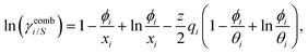
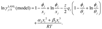
The solubility of greenhouse gases was recently reported using a new model here referred as the COSMOSAC-LANL25 activity coefficient model. This model includes two terms: a 3-suffix Margules (3sM)20,21 function as a quantitative measurement of inherent asymmetric interaction present in a solution due to the hydrogen bond interaction, strong dispersion and coulombic interaction and the long-range Staverman–Guggenheim22,23(SG) combinatorial interaction due to the size and shape differences between solute and solvent molecules. We will work in the regime of low solubility where γLANLi/S ≥ 1, i.e.; lnγLANLi/S ≥ 0. Hence, we invoke a new asymmetric interaction in terms of the “LANL” activity coefficient model| | | ln(γLANLi/S) = ln(γcombi/S) + ln(γasymi/S), | (1) |
where we define ln(γasymi/S) = (ΔGasymi/S − ΔGasymi/i)/RT which is the difference between the asymmetric interactions in a mixture (i/S) and in pure state (i/i), which represents the solvation free energy change in terms of solute and solvent interactions when a solute particle goes into a fixed position in solution from a fixed position in its ideal state. Since the “LANL” activity coefficient model has asymmetric interaction (ln(γasymi/S)), the total activity coefficient (ln(γLANLi/S)) model is also called an asymmetric model. For pure species, the asymmetric interaction is zero, ΔGasymi/i = 0, and hence, ln(γasymi/S) = (ΔGasymi/S)/RT = (ΔGsolvi/S − ΔGsolvi/i)/RT = (ΔGsolv)/RT. In COSMOSPACE26,27 (the pictorial representation is shown in Fig. 1), it can be seen that the activity coefficient due to the asymmetric interaction is equal to the activity coefficient due to the short range residual interaction (γresiduali/S) at infinite dilution (xsolute=i → 0, xsolvent=j → 1). In COSMOSPACE, the activity coefficient can be written in terms of the segment interaction as| | 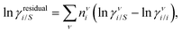 | (2) |
where i stands for pure compound, ν stands for the different type of segment, and ni stands for the number of segments of type ν and say, (lnγνi/S − lnγνi/i) = lnγνi/S(asym). The asymmetric interaction mentioned above can be written in terms of asymmetric segment interaction| | 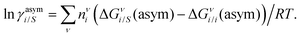 | (3) |
where ΔGνi/i(asym)/RT = 0 for an ideal case, so  . Since for similar types of segments the concept of asymmetric interaction between segments does not exist, so lnγνi/i(asym) will vanish and therefore the equation will be reduced to
 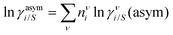 . In this model, we used the 3-suffix Margules function to capture the asymmetric interaction in terms of Margules parameters. Therefore, the expression of the excess Gibbs energy due to the asymmetric interaction can be written as
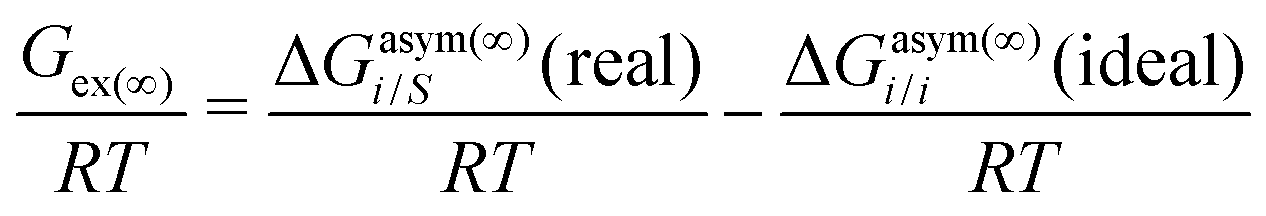
| | | Gex = ΔGasymi/S(real) − ΔGasymi/i(ideal) = x1x2(A21x1 + A12x2), | (4) |
where x1 and x2 are the mole fractions for solute and solvent molecules in a binary mixture and A21 and A12 are the Margules parameters. For asymmetric solutions when A12 ≠ A21 and when they are equal (A12 = A21), the solution is symmetric reducing eqn (4) to the 2-suffix Margules function. A pictorial representation showing how these Margules parameters are obtained is given in Fig. 1.
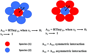 |
| | Fig. 1 A cartoon representation of asymmetric interaction in a binary mixture at infinite dilution. | |
By differentiating eqn (4) with respect to the mole number for species 1 and 2,27,28 one can get the asymmetric activity coefficient
| |  | (5) |
where
n is the total mole number and
ni is the mole number of species (
i = 1, 2), and
xi = mole fraction =
ni/
n of
i-th species. Therefore the expressions for the activity coefficients for both species 1 and 2 present in the binary mixture solution are
| | 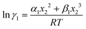 | (6) |
| | 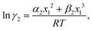 | (7) |
where
α1 = (2
A21 −
A12),
β1 = (2
A12 − 2
A21),
α2 = (2
A12 −
A21), and
β2 = (2
A21 − 2
A12). These parameters are calculated from the activity coefficients of species 1 in species 2 and species 2 in species 1 under infinite dilute conditions.
20 The differentiation of
eqn (4) and the derivation of the 2-suffix Margules function from the 3-suffix Margules function are given in Sections 1 and 2, respectively, in the ESI.
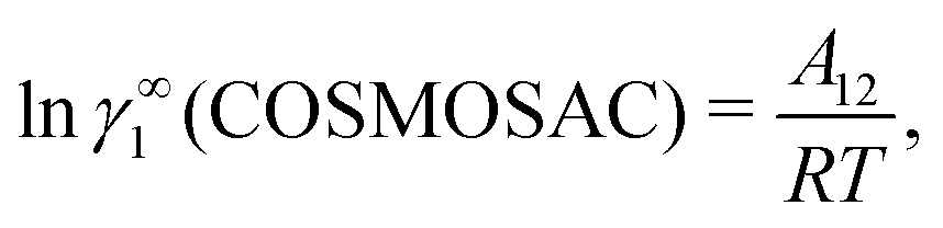
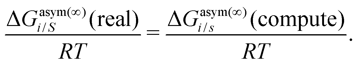
† Within the 3-suffix Margules law, at infinite dilution
eqn (6) and (7) can be written as ln
γasymi/S =
A/
RT, where
A is equal to
RTln
γ∞i/S and which is either
A12 (accounts solubility of species 1 in 2) or
A21 (accounts solubility of species 2 in 1). A description has been given in Appendix A. Therefore,

. Hence, one can implicitly express the residual interaction within the asymmetric 3-suffix Margules function for a binary mixture. We use the activity coefficient at infinite dilution (
γ∞) calculated using the COSMOSAC-2013
24,29 model for all binary mixture solutions used in this work. The reasons for using the COSMOSAC-2013 model are as follows (i) this is the only COSMOSAC model whose parameters are optimized over a large data set for ADF calculation,
24 (ii) this is the only COSMOSAC model which includes a sophisticated dispersion interaction along with a modified residual and combinatorial term and also, (iii) this model holds an exact expression for the segment chemical potential that satisfies over all boundary conditions, and the resulting equation for the activity coefficient obeys the Gibbs–Duhem relationship to maintain thermodynamic consistency. Therefore, the basic background of the proposed model is based on the COSMOSAC-2013 model in this study. The concept of the COSMOSPACE has been used to explain the implicit definition of the residual interaction within the asymmetric term present in the “LANL” activity coefficient model within the COSMO-RS framework. The
A12 and
A21 cases have been shown for a spherical solute and solvent molecules in
Fig. 1 which is in a hypothetical COSMOSPACE.
It is already known that the 3-suffix Margules function usually represents a less regular and therefore less asymmetric solution.1 Since solubility is an entropy driven phenomenon the effect of entropy comes from size and shape differences between the solute and solvent species. To consider the effect due to the different sizes and shapes of the solute and solvent species (long range interaction) the Staverman–Guggenheim (SG)5,22–24,30 combinatorial term has been used here
| |  | (8) |
with
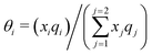
and
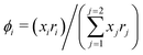
, where
xi is the mole fraction of component
i;
ri and
qi are the normalized volume and surface area parameters for species
i and
z is the coordination number equal to 10.
zqi represents the number of nearest-neighbor sites to one of the solute and solvent molecules. In this model for the combinatorial term only the surface area
qi has been normalized with
q0 = 79.53. A detailed description of this SG form has been given in Section 3 in the ESI.
† After adding the terms for combinatorial and asymmetric interactions described above, we obtain the expression for the activity coefficient for solute (
i) and solvent (
j) species in solution as:
| | 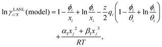 | (9) |
and
| |  | (10) |
Eqn (9) and (10) are called the “LANL” activity coefficient model in the rest of the paper and in some cases the model is referred as the COSMOSAC-LANL model as we imported Margules parameters from the COSMOSAC-2013 model. At infinite dilution (xsolute=i → 0, xsolvent=j → 1) the two models COSMOSAC-LANL and COSMOSAC-2013 are connected by
| | | lnγi/S(COSMOSAC-LANL) − lnγi/S(COSMOSAC-2013) = lnγi/S(comb). | (11) |
At, ln
γi/S(comb) < 0, ln
γi/S(COSMOSAC-LANL) < ln
γi/S(COSMOSAC-2013) since a similar combinatorial term has been used in both the models and based on the derivation in Appendix A, the effect of the combinatorial term thus has been counted here twice as a consequence of the proposed model. Therefore to overcome the effect due to the combinatorial term, we change
eqn (9) and (10) based on our proposed assumption on the low solubility region (
γLANLi/S ≥ 1) to
| | 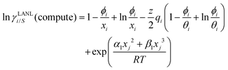 | (12) |
for the solute species,
| | 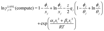 | (13) |
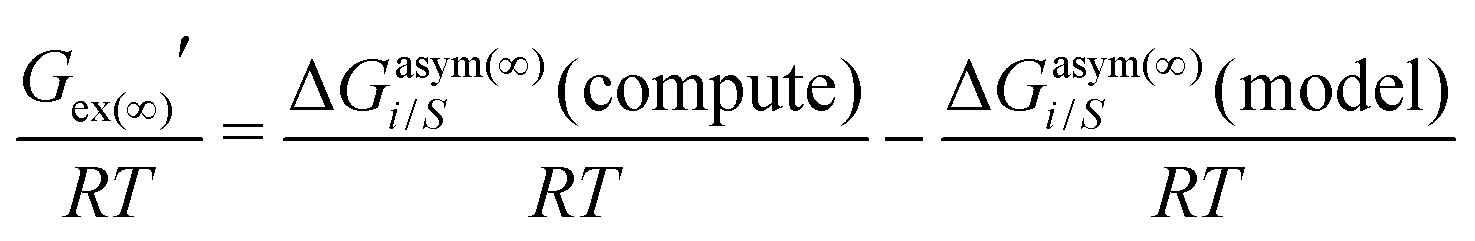
for solvent species, respectively. We have defined
eqn (9) and (10) as ln
γLANLiorj/S(model) and
eqn (12) and (13) as ln
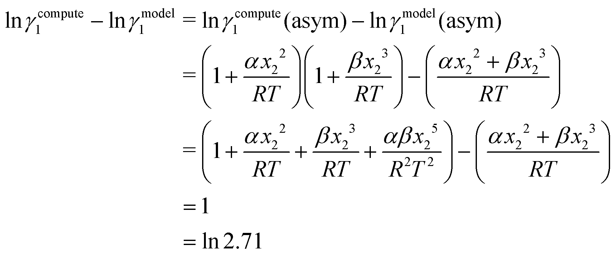
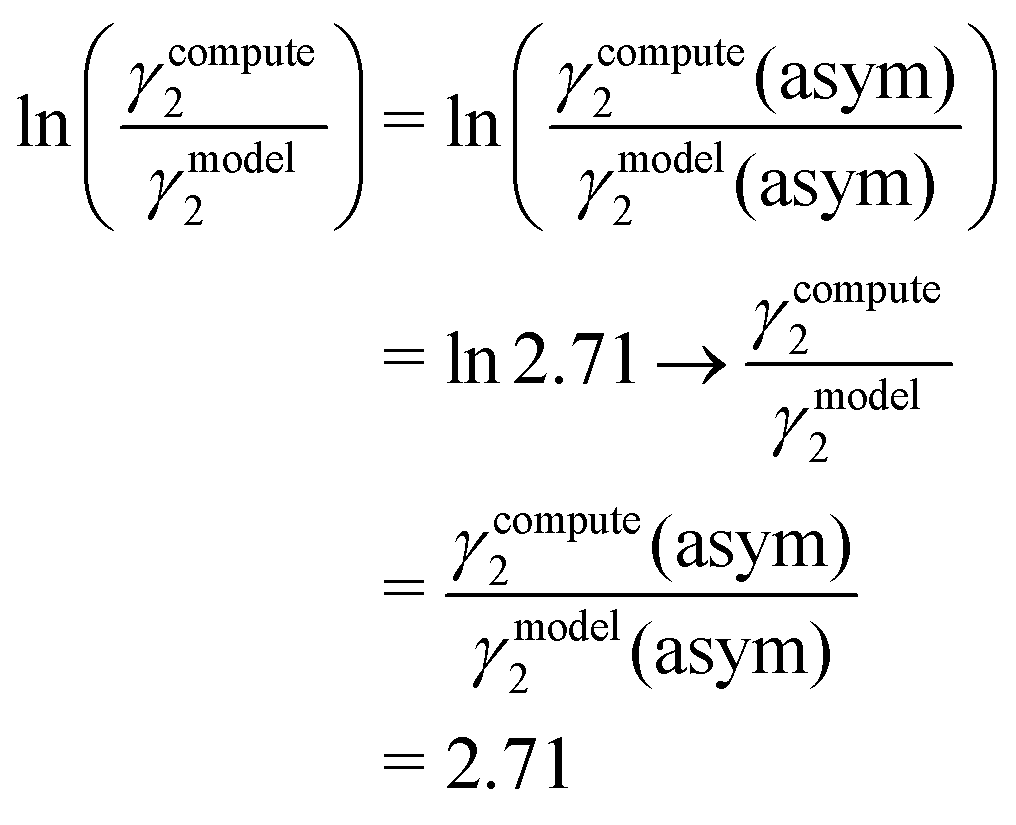
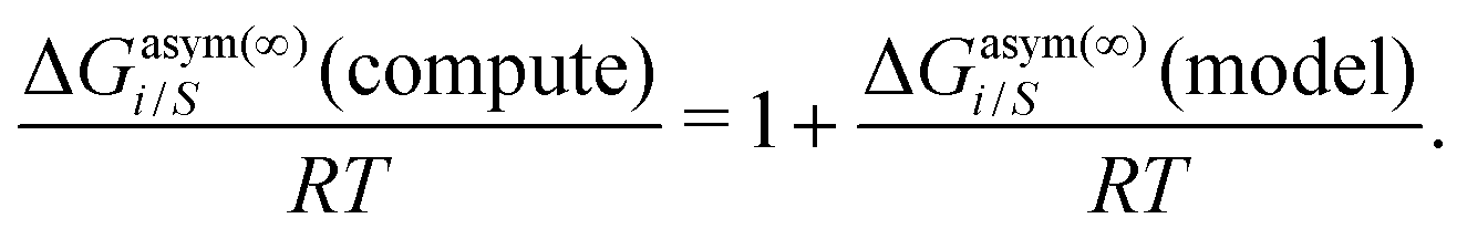
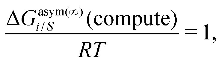
γLANLiorj/S(compute) for species 1 and 2, respectively. The COSMO volume and surface for the pure species obtained from the COSMOSAC-2013 model have been used to calculate the combinatorial term. Since we use the same combinatorial term in the model for the asymmetric interaction due to the size and shape differences between the solute and solvent species, we changed the asymmetric contribution coming from the residual interaction by changing the standard state of the
γasymi/S from 1 to 2.71 and hence by making the asymmetric contribution slightly more asymmetric towards the less solubility region based on our proposed assumption at the very beginning of this model
i.e.;
γLANLi/S ≥ 1. Therefore, we focus on obtaining a more accurate activity coefficient at infinite dilution. A relationship between ln
γmodeli/S and ln
γcomputei/S has been established by
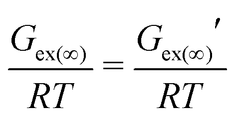
| | | lnγi/S(real) = lnγi/S(compute) = 1 + lnγi/S(model), | (14) |
for the solute species in a binary mixture. The details of the derivation has been given in Appendix B.
Eqn (14) is valid when the binary system is approaching
x1 → 1;
x2 → 0 for a species. The limit mentioned for
eqn (14) holds the region
x1 → 0;
x2 → 1 for a species within it according to the proposed model (Appendix B). The other thermodynamic properties like excess Gibbs energy, free energy of mixing, variation of the logarithm of activity coefficient with the solute mole fraction for the whole range of concentrations obtained using
eqn (12) and (13) are calculated using the relation ln
γi/S(model) = ln
γi/S(compute)/2.71 for
γ scale 0 to 1. The present COSMOSAC-LANL model is applicable only to the mixture system (such as CO
2 in ILs and CH
4 in ILs). The structural and other physical properties of the pure species have been computed using the ADF-COSMOSAC-2013 model. To verify the asymmetric solution model, we computed various thermodynamic properties (such as
Gex and Δ
Gmix) and correlations between ln
γLANLi, ln
γLANLj and

with varying mole fractions of the solute species.
1 We calculated the total excess Gibbs energy (
Gex) for the binary system using the equation
| | | Gex = RT(xilnγLANLi/S + xjlnγLANLj/S), | (15) |
and the free energy of mixing for the binary mixture using
| | | ΔGmix = RT(xilnxi + xjlnxj + xilnγLANLi/S + xjlnγLANLj/S), | (16) |
where ln
γLANLi/S and ln
γLANLj/S are obtained from
eqn (12) and (13).
At infinite dilution, Henry's constant is related to the infinite dilution activity coefficient and the fugacity of pure gas,1,2
| | 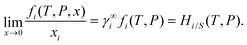 | (17) |
The solubility of gas molecules in ionic liquids can be measured by taking the inverse of Henry's constant at a partial pressure of 1 bar,
i.e.,
xi = 1/
Hi/S. Henry's constant is directly related to the free energy of solvation (Δ
G∞solv) which is defined as the change in Gibbs energy upon transferring a gas molecule from the pure gaseous phase at some standard pressure
p0 to the infinite solution and they are related to each other as follows
| | | ΔG∞solv = RTlnHi/S. | (18) |
The fugacity of the gas molecule was calculated following the relation described in the work of Lin
et al.,
31 which is
| | | lnfi(T,P) = Ai + Bi/T + CilnT + DiTEi. | (19) |
The computational details of the parameters
Ai,
Bi,
Ci,
Di and
Ei are given in the work of Lin
et al.31 This thermodynamic property is a function of solute. The activity coefficients at infinite dilution calculated using the asymmetric model and the fugacity calculated using the above relations have been used to calculate the solubility of CO
2 in ionic liquids. We have calculated the activity coefficients at infinite dilution from the new COSMOSAC-LANL model which has been discussed in detail in the previous section.
3 Computational details
All the COSMO19 files for CO2, CH4 and ionic liquids have been generated using the Amsterdam Density Functional software version 2016.24,32 The initial structures of each gas and ionic liquid have been drawn in ADFview. Then they have been relaxed using a simple UFF method already implemented in ADF2016. Using the final geometry resulting from the UFF calculations, the rest of the calculations have been performed. The geometry optimization was performed using the generalized gradient approximation (GGA) with the BP exchange correlation functional. The zero order regular approximation (ZORA) method was used for calculating the relativistic effect. The TZP basis set for small frozen core and Becke integration with the spline Zlm fit for density fitting have been used in ADF for each molecule followed by the post COSMOSAC calculation already implemented in ADF for the calculation of the σ profile of each molecule. It should be noted that the parameters used in the COSMOSAC-201324 model are not optimized for ionic liquids. So, in our calculations we simply used those parameters which were optimized for the simple organic molecules and their systems in the ADF software for the COSMOSAC-2013 model.24 The details of quantum COSMO settings have been given in the paper on the COSMOSAC-2013 model of Xiong et al.24 Each ionic liquid has been treated as a single intact ionic liquid molecule in the quantum COSMO calculation since it is already known from the work of Kirchner et al.33,34 that the total charge of each species in an ionic liquid is always less than 1 due to the intermolecular charge transfer between the cation and anion. To ensure this fact, we calculated the σ profile for 18 ionic liquids by first treating them as (case I) single intact molecules and then as (case II) separate cation and anion moieties and calculated their σ profiles. The σ profile (pσ) is defined as the probability of finding a segment of the COSMO surface with charge density σ.35 In most cases, significant differences in their σ profile for the different types of treatments (case I) and (case II) of ionic liquids were observed as shown in Fig. 2. The results for case I and case II for 24 ionic liquids are shown in Table 1. The solubility calculations have been done using ADF-COSMOSAC-2013. In case I, each ionic liquid has been treated as a single molecule, therefore their solutions have been treated as a binary mixture. The solution has been treated as a ternary mixture for case II. Therefore, necessary calculations have been done to convert the solubility data by dividing γ∞ by 2. This has been discussed in Section 4 in the ESI.† We notice that the solubility results vary significantly for the different treatments of the ionic liquid using the COSMOSAC-2013 model. The calculated average absolute relative deviations (AARD) for case I and case II are 31% and 63%, respectively.
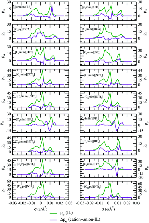 |
| | Fig. 2
σ profiles and their differences for two different treatments of ionic liquids. | |
Table 1 The effect of different treatments of ionic liquids on activity coefficient at infinite dilution (γ∞i/S). The solubility calculations have been performed using the COSMOSAC-2013 model. The solubility data are in mole fraction unit. Case I is singe intact molecule and Case II is separate cation and anion
| Numbers |
Ionic liquids |
T (K) |
Experimental |
Case I |
Case II |
| 1 |
[C2mim][BF4] |
298 |
0.012 |
0.016 |
0.022 |
| 2 |
[C2mim][EtSO4] |
293.15 |
0.015 |
0.033 |
0.036 |
| 3 |
[C4py][DCA] |
298.15 |
0.016 |
0.025 |
0.040 |
| 4 |
[C4dmim][PF6] |
298.1 |
0.016 |
0.026 |
0.032 |
| 5 |
[C4dmim][BF4] |
298.1 |
0.016 |
0.026 |
0.033 |
| 6 |
[C4py][F3Ac] |
298.15 |
0.018 |
0.025 |
0.041 |
| 7 |
[C4mim][BF4] |
298.1 |
0.018 |
0.021 |
0.026 |
| 8 |
[C4mim][DCA] |
298 |
0.018 |
0.028 |
0.028 |
| 9 |
[C4mim][PF6] |
298.1 |
0.019 |
0.026 |
0.027 |
| 10 |
[C2mim][OTf] |
298.2 |
0.019 |
0.019 |
0.023 |
| 11 |
[C3mim][PF6] |
298.1 |
0.019 |
0.018 |
0.023 |
| 12 |
[C4mim][OTf] |
298.15 |
0.022 |
0.025 |
0.030 |
| 13 |
[C2dmim][NTf2] |
298.1 |
0.025 |
0.029 |
0.038 |
| 14 |
[C4mpyr][NTf2] |
298.15 |
0.026 |
0.038 |
0.044 |
| 15 |
[C3mim][NTf2] |
298.1 |
0.027 |
0.032 |
0.039 |
| 16 |
[C2mim][NT2] |
298.1 |
0.028 |
0.029 |
0.035 |
| 17 |
[C4mim][NTf2] |
298.1 |
0.030 |
0.035 |
0.042 |
| 18 |
[C6mpy][NTf2] |
298 |
0.030 |
0.039 |
0.050 |
| 19 |
[C4py][NTf2] |
298.15 |
0.031 |
0.033 |
0.054 |
| 20 |
[C8mim][NTf2] |
298.1 |
0.033 |
0.041 |
0.052 |
| 21 |
[C6mim][NTf2] |
298.06 |
0.034 |
0.041 |
0.046 |
| 22 |
[C8py][NTf2] |
298.15 |
0.036 |
0.043 |
0.050 |
| 23 |
[C10py][NTf2] |
298.15 |
0.036 |
0.049 |
0.054 |
| 24 |
[C8h4f13][NTf2] |
298.04 |
0.040 |
0.040 |
0.056 |
|
|
|
|
AARD |
— |
— |
0.31 |
0.63 |
For solubility calculations in ionic liquids, eqn (17) was solved for a partial pressure of 1 bar. In the present calculation, the solubility of two greenhouse gases mainly CO2 and CH4 has been calculated at different temperatures and at constant low partial pressure (1 bar) of the gases. All Margules parameters (A12) and (A21) were calculated using the ADF-COSMOSAC-2013 model at xi → 0, xj → 1 and xj → 0, xi → 1, for species i and j, respectively. After getting those parameters, we calculated the solubility and other equilibrium thermodynamical properties stated in eqn (15)–(17) (Gex, ΔGmix and solubility isotherm) for all binary mixtures used in this study. The calculated values of asymmetric interactions along with the calculated combinatorial term at infinite dilution have been given in Table 2. A minimum criterion has been established for when to apply eqn (9) in place of eqn (12) using the relationship in eqn (14) and that is lnγasymi/S(compute) = 1 (Appendix C). Only the ionic liquid ([Eohmim][BF4]) showing the lowest solubility of CO2 is found to satisfy the above condition.
Table 2 lnγCOSMOSAC-2013i/S, lnγasymi/S and lnγcombinatoriali/S at infinite dilution for CO2 solubility in 33 room temperature ionic liquids (RTILs)
| Numbers |
Ionic liquids |
lnγCOSMOSAC-2013i/S |
lnγasymi/S = (α + β)/RT |
lnγcombinatoriali/S |
| 1 |
[Eohmim][BF4] |
0.78 |
0.78 |
−0.56 |
| 2 |
[C2mim][BF4] |
−0.01 |
−0.01 |
−0.69 |
| 3 |
[C2mim][DCA] |
0.03 |
0.03 |
−0.66 |
| 4 |
[C2mim][EtSO4] |
−0.64 |
−0.64 |
−0.81 |
| 5 |
[C4py][DCA] |
−0.46 |
−0.46 |
−0.82 |
| 6 |
[C4dmim][PF6] |
−0.51 |
−0.51 |
−0.95 |
| 7 |
[C4dmim][BF4] |
−0.51 |
−0.51 |
−0.83 |
| 8 |
[C4py][F3Ac] |
−0.50 |
−0.50 |
−0.85 |
| 9 |
[C4mim][BF4] |
−0.28 |
−0.28 |
−0.79 |
| 10 |
[C4mim][DCA] |
−0.60 |
−0.60 |
−0.85 |
| 11 |
[C8mim][BF4] |
−0.71 |
−0.71 |
−1.02 |
| 12 |
[C4mim][PF6] |
−0.51 |
−0.51 |
−0.85 |
| 13 |
[C2mim][OTf] |
−0.21 |
−0.21 |
−0.80 |
| 14 |
[C3mim][PF6] |
−0.14 |
−0.14 |
−0.79 |
| 15 |
[C4mim][OTf] |
−0.47 |
−0.47 |
−0.91 |
| 16 |
[C6tma][NTf2] |
−1.14 |
−1.14 |
−1.59 |
| 17 |
[C2dmim][NTf2] |
−0.63 |
−0.63 |
−0.98 |
| 18 |
[C4mpyr][NTf2] |
−0.90 |
−0.90 |
−1.15 |
| 19 |
[C3mim]NTf2] |
−0.72 |
−0.72 |
-1.08 |
| 20 |
[C2mim][NTf2] |
−0.63 |
−0.63 |
−1.05 |
| 21 |
[C4mim][NTf2] |
−0.81 |
−0.81 |
−1.10 |
| 22 |
[C6mpy][NTf2] |
−−0.90 |
−0.90 |
−1.10 |
| 23 |
[C4py][NTf2] |
−0.76 |
−0.76 |
−1.12 |
| 24 |
[C10mim][NTf2] |
−1.07 |
−1.07 |
−1.31 |
| 25 |
[C8mim][NTf2] |
−0.97 |
−0.97 |
−1.25 |
| 26 |
[C6mim][NTf2] |
−0.96 |
−0.96 |
−1.23 |
| 27 |
[C8py][NTf2] |
−1.03 |
−1.03 |
−1.22 |
| 28 |
[C10py][NTf2] |
−1.15 |
−1.15 |
−1.36 |
| 29 |
[C12py][NTf2] |
−1.18 |
−1.18 |
−1.38 |
| 30 |
[C1c4pyrro][eFAP] |
−1.03 |
−1.03 |
−1.24 |
| 31 |
[C8h4f13][NTf2] |
−0.95 |
−0.95 |
−1.30 |
| 32 |
[C6mim][eFAP] |
−1.17 |
−1.17 |
−1.33 |
| 33 |
[P66614][eFAP] |
−1.62 |
−1.62 |
−1.85 |
If a solution obeys Raoult's law, it is known as an ideal solution. Any positive and negative deviation from Raoult's law (p vs. x plot) represents a regular solution. If the deviation from Raoult's law is more, the solution will show asymmetric behavior either in the positive or in the negative direction in the p vs. x plot. Based on the amount of the deviation, it will be known as the symmetric (less deviation from Raoult's law) or asymmetric (more deviation from Raoult's law) regular solution. In the present model, the residual interaction presents implicitly within the asymmetric interaction of the 3-suffix Margules function type. Later, by combining the 3-suffix Margules function with the SG term, we consider all types of short range and long range interactions present in a binary mixture. Such explicit treatment of the asymmetric interaction only between the solute and solvent species allows us to explain any positive or negative deviation (asymmetric interaction) from Raoult's law using the other derivations given in Appendix A to Appendix C in the main article. The 3-suffix Margules function often represents the less regular solution. The less regular behavior of the ADF-COSMOSAC-2013 model has been shown in Table 2. If the ADF-COSMOSAC-2013 model could predict the strong regular solution behavior of the CO2/IL binary mixture, then γ∞(COSMOSAC-2013) ≠ γ∞(3-suffix Margules function). Since γ∞(COSMOSAC-2013) = γ∞(3-suffix Margules function) as shown in Table 2, the COSMOSAC-2013 model presents a less regular solution and thus a less asymmetric solution model for CO2 solubility in ionic liquids.
For thermodynamic consistency it is important to point out that the differentiation must satisfy the Gibbs–Duhem equation
| | x1dlnγ1 + x2d![[thin space (1/6-em)]](https://www.rsc.org/images/entities/i_char_2009.gif) lnγ2 = 0. lnγ2 = 0. | (20) |
The numerical differentiation has been done on a set of activity coefficient data for varying mole fractions for both solute and solvent molecules. An analytical solution of 3-suffix Margules functions and a demonstration of the numerical differentiation for two different systems have been given in Sections 5 and 6, respectively, in the ESI.
† We used
eqn (12) to calculate the solubility of CH
4 to check the selectivity between CO
2 and CH
4 gases because the asymmetric interactions will be more for CH
4 gas in ILs than the asymmetric interactions observed for CO
2 in ILs in the regime
γLANLi/S ≥ 1,
i.e.; ln
γLANLi/S ≥ 0. This is indicated from their very high values of fugacity calculated using
eqn (19) and lower molecular weights with respect to CO
2 (
i.e.;
mCO2 >
mCH4) given in
Table 3. The fugacity is inversely related to the solubility of the gas according to
eqn (17).
Table 3 Calculated fugacities of CO2 and CH4 at different temperatures using eqn (19)31
| Temperature (K) |
f
CO2 (bar) |
f
CH4 (bar) |
| 298 |
64.09 |
731.28 |
| 298.15 |
64.31 |
733.89 |
| 303.15 |
71.98 |
826.58 |
| 313.15 |
89.47 |
1049.69 |
4
σ profile of ionic liquids and their conformational dependence
The impact of different conformations of ionic liquids on the other physical and thermodynamical properties has been looked at and confirmed for 18 different ionic liquids for two different conformers. To check any kind of such dependency, we performed two types of quantum COSMO calculations: (i) the quantum COSMO calculations have been directly performed on the geometry drawn in ADFview, followed by a relaxation using the UFF method followed by the ADF-COSMOSAC-2013 calculation without any a priori separate geometry optimization and analytical frequency calculation and (ii) the quantum COSMO calculations have been directly performed on the geometry drawn in ADFview, followed by a relaxation using the UFF method followed by the ADF-COSMOSAC-2013 calculation with a priori separate geometry optimization and analytical frequency calculation. The conformation generated following the first method (i) is known as Conf1 and the conformation generated following the second method (ii) is known as Conf2. Using these schemes, we first did our quantum calculations for geometry optimization followed by the calculations of the analytical frequency to check any presence of the imaginary frequency in the calculated analytical frequency and thus to ensure that the ground state global geometry has been reached. A similar type of quantum settings has been chosen for the calculations because the geometry optimization in the gas phase is already included in the COSMOSAC-2013 model in ADF. Therefore to maintain the parity between these two calculations, the same quantum setting has been selected for the geometry optimization followed by the analytical frequency calculations. The quantum setting for the geometry optimization and analytical frequency calculation have been given in Table 4. The difference between the σ profile of the conformations Conf1 and Conf2 (Δpσ) along with the σ profile of the conformation Conf2 (pσ) has been shown in Fig. 3. The calculated analytical frequency for 18 different ionic liquids has been shown in Fig. S1 in the ESI.† All 18 ionic liquids studied along with their COSMO surface points have been given in Fig. S2–S4 (ESI†) and the different conformers Conf1 and Conf2 have been shown in Fig. S5 in ESI.† Almost for all cases, we find that the difference between the σ profiles (Δpσ) passes through zero without showing any significant changes except for the ionic liquid containing [BF4]− and [PF6]− anion. The calculated solubility and activity coefficient for 18 different ionic liquids for two different conformers have been given in Table 5.
Table 4 The details of geometry optimization and frequency calculations
| Basis set |
TZP |
| Frozen Core |
Small |
| Task |
GO & Frequency calculation |
| XC |
Becke Perdew |
| Frequency |
Analytical |
| Numerical quality |
Excellent |
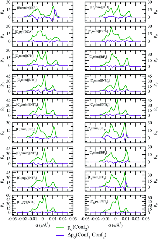 |
| | Fig. 3
σ profiles and their differences for two different conformations of ionic liquids. | |
Table 5 The effect of different conformations of ionic liquids on activity coefficient at infinite dilution (γ∞i/S). The all solubility calculations have been performed using the COSMOSAC-2013 model. The solubility data are in mole fraction unit
| Numbers |
Ionic liquids |
γ
∞
i/S
|
γ
∞
i/S
|
| Conf1 |
Solubility |
Conf2 |
Solubility |
| 1 |
[Eohmim][BF4] |
2.18 |
0.007 |
1.12 |
0.014 |
| 2 |
[C2mim][OTf] |
0.81 |
0.019 |
0.82 |
0.019 |
| 3 |
[C4py][DCA] |
0.63 |
0.025 |
0.61 |
0.025 |
| 4 |
[C4mim][DCA] |
0.55 |
0.028 |
0.57 |
0.027 |
| 5 |
[C4mim][OTf] |
0.63 |
0.025 |
0.60 |
0.026 |
| 6 |
[C8mim][BF4] |
0.49 |
0.032 |
0.49 |
0.032 |
| 7 |
[C3mim][NTf2] |
0.49 |
0.032 |
0.49 |
0.032 |
| 8 |
[C2mim][NTf2] |
0.53 |
0.029 |
0.53 |
0.029 |
| 9 |
[C4dmim][NTf2] |
0.43 |
0.036 |
0.44 |
0.035 |
| 10 |
[C4mim][NTf2] |
0.45 |
0.035 |
0.47 |
0.033 |
| 11 |
[C4mim][BF4] |
0.76 |
0.021 |
0.73 |
0.022 |
| 12 |
[C4dmim][PF6] |
0.61 |
0.027 |
0.61 |
0.027 |
| 13 |
[C2dmim][NTf2] |
0.54 |
0.030 |
0.50 |
0.032 |
| 14 |
[C2mim][BF4] |
0.99 |
0.016 |
0.95 |
0.017 |
| 15 |
[C3mpy][NTf2] |
0.43 |
0.037 |
0.43 |
0.037 |
| 16 |
[C8mim][PF6] |
0.50 |
0.033 |
0.44 |
0.037 |
| 17 |
[C10py][NTf2] |
0.33 |
0.049 |
0.34 |
0.048 |
| 18 |
[C12py][NTf2] |
0.32 |
0.051 |
0.32 |
0.051 |
From our calculations, it is clear that the conformational dependency on the σ profile and hence on the activity coefficient at infinite dilution is very negligible except for the ionic liquid ([Eohmim][BF4]). The reason behind this observation has been explained in Section 5.1. This observation is also reflected on their solubility data given in Table 5 for two different conformers. Since for 18 different ionic liquids, we did not observe any significant changes in the solubility for two different conformers, therefore for the remaining 15 ionic liquids we did our calculations following Conf1 case.
A similar approach to the conformational dependency on the σ profile of ionic liquid has been already proposed to model the solubility of metal complexes in ionic liquids using the COSMOSAC-LANL model.25 In case of the metal complex solubility in ionic liquids, ΔGex due to the combinatorial term is significant and higher with respect to the combinatorial interaction between the CO2 and the ionic liquid. The COSMO volume and surface of a transition metal complex is almost ∼10 times higher than the same for CO2 and CH4 gases. These differences in the COSMO volume and surfaces will effect the combinatorial interaction in those solid–liquid equilibria significantly. We notice that the combinatorial interaction between the CO2 gas and the ionic liquid has a stabilizing effect while the same between the metal complex and the ionic liquid has a destabilizing effect on the solubility. The result is shown in Table 6.
Table 6 The residual and combinatorial interaction in 33 binary mixtures at 1 bar partial pressure
| Numbers |
Ionic liquids |
Temperature (K) |
γ (residual) |
γ (SG comb) |
| 1 |
[Eohmim][BF4] |
303.15 |
2.44 |
0.57 |
| 2 |
[C2mim][BF4] |
298 |
2.76 |
0.5 |
| 3 |
[C2mim][DCA] |
303.1 |
2.92 |
0.52 |
| 4 |
[C2mim][EtSO4] |
293.15 |
1.71 |
0.45 |
| 5 |
[C4py][DCA] |
298.15 |
1.89 |
0.44 |
| 6 |
[C4dmim][PF6] |
298.1 |
1.83 |
0.39 |
| 7 |
[C4dmim][BF4] |
298.1 |
1.83 |
0.43 |
| 8 |
[C4py][F3Ac] |
298.15 |
1.84 |
0.43 |
| 9 |
[C4mim][BF4] |
298.1 |
2.16 |
0.45 |
| 10 |
[C4mim][DCA] |
298 |
1.73 |
0.43 |
| 11 |
[C8mim][BF4] |
303 |
1.64 |
0.36 |
| 12 |
[C4mim][PF6] |
298.1 |
2.12 |
0.43 |
| 13 |
[C2mim][OTf] |
298.2 |
2.27 |
0.45 |
| 14 |
[C3mim][PF6] |
298.1 |
2.42 |
0.45 |
| 15 |
[C4mim][OTf] |
298.15 |
1.89 |
0.4 |
| 16 |
[C6tma][NTf2] |
303.15 |
1.39 |
0.2 |
| 17 |
[C2dmim][NTf2] |
298.1 |
1.7 |
0.37 |
| 18 |
[C4mpyr][NTf2] |
298.15 |
1.5 |
0.32 |
| 19 |
[C3mim]NTf2] |
298.1 |
1.63 |
0.34 |
| 20 |
[C2mim][NTf2] |
298.1 |
1.71 |
0.35 |
| 21 |
[C4mim][NTf2] |
298.1 |
1.56 |
0.33 |
| 22 |
[C6mpy][NTf2] |
298 |
1.55 |
0.33 |
| 23 |
[C4py][NTf2] |
298.15 |
1.6 |
0.33 |
| 24 |
[C10mim][NTf2] |
303.4 |
1.4 |
0.27 |
| 25 |
[C8mim][NTf2] |
298.1 |
1.45 |
0.29 |
| 26 |
[C6mim][NTf2] |
298.06 |
1.46 |
0.29 |
| 27 |
[C8py][NTf2] |
298.15 |
1.42 |
0.3 |
| 28 |
[C10py][NTf2] |
298.15 |
1.37 |
0.26 |
| 29 |
[C12py][NTf2] |
298.15 |
1.35 |
0.25 |
| 30 |
[C1c4pyrro][eFAP] |
303.16 |
1.44 |
0.29 |
| 31 |
[C8h4f13][NTf2] |
298.04 |
1.47 |
0.27 |
| 32 |
[C6mim][eFAP] |
298.6 |
1.36 |
0.27 |
| 33 |
[P66614][eFAP] |
303.19 |
1.21 |
0.16 |
5 Results and discussion
5.1 Solubility isotherm and σ profile
The solubility of two gases in room temperature ionic liquids has been calculated using| | | xi = γ∞ifi(T,P) = Hi/S(T,P). | (21) |
at infinite dilute condition. The all quantities present in the above equation have been explained in eqn (17) in Section 2. The solubility isotherm has been calculated in all cases by using pi = xiγ∞ifi(T,P),31 where γ∞i is the activity coefficient at infinite dilution, fi is the fugacity and pi is the pressure. The results have been discussed in the following paragraphs.
The solubility isotherms for CO2 in [C4mim][NTf2] ionic liquids at four different temperatures are shown in Fig. 4 along with the experimental results.36 From the solubility isotherm it is confirmed that the model works up to ∼6 bar partial pressure very well for CO2 solubility in the ionic liquid. Similar calculations have been done for the solubility of CH4 gas molecules in [C4mim][PF6] at room temperature (298 K) as shown in Fig. 5. The calculated results are in good agreement with the experimental results at a low partial pressure (1 bar) and hence, in the low solubility region for both CO2 and CH4 gas.
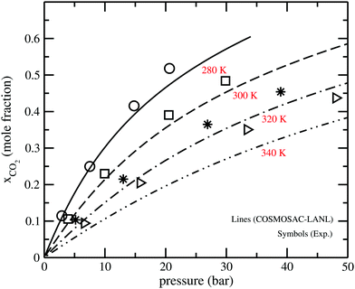 |
| | Fig. 4 The solubility isotherm for CO2 in the [C4mim][NTf2] ionic liquid. The experimental results have been taken from the work of Kazakov et al.36 | |
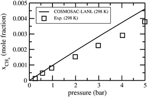 |
| | Fig. 5 Solubility isotherm for CH4 for ionic liquid [C4mim][PF6]. The experimental results have been taken from the work of Lin et al.31 | |
In this study we have taken the σ profile for each molecule calculated using the COSMO setting mentioned in the work of Xiong et al.24Fig. 6 shows the calculated σ profile of three types of ionic liquids categorized as maximum ([P66614][eFAP]),37 medium ([C2dmim][NTf2], [C4mpyr][NTf2]) and least ([Eohmim][BF4]) CO2 absorber. COSMOSAC24,38 classifies the segment of the COSMO surface into three categories: (a) non hydrogen bonding, (b) hydrogen bonding from the OH group and, (c) hydrogen bonding from other than the OH group. A Gaussian like function has been considered to express the probability of hydrogen bonding segments
| | 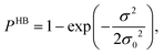 | (22) |
where
σ is the screening charge density and
σ0 is equal to 0.007 e Å
−2 for the Gaussian distribution. The relation between them is
pσ(HB) =
pσ(OH⋯OH) +
pσ(OH⋯OT) and thus
pσ(total) =
pσ(HB) +
pσ(NHB), where
pσ(NHB) is the sigma profile due to the non-hydrogen bonded group.
and
, where
Ai is the COSMO surface. The details are given in the work of Xiong
et al.24 The molecules having the ability to form intermolecular hydrogen bonds between the hydroxyl (OH) group of the cation and the FB group of BF
4− are the least CO
2 absorbers because the physical absorption of CO
2 molecules in those ionic liquids will cost high Gibbs free energy of cavity formation at the expense of breaking of intermolecular (H⋯F) hydrogen bonds. Such kind of (OH⋯OT) bond formation has been shown in
Fig. 6; plot (a) indicated by a blue line, the smaller amount of (OH⋯OH) is indicated by a green line and the total of (OH⋯OT) and (OH⋯OH) is indicated by a red line and the total
σ profile
ptotal(
σ) is indicated by a black line. Also, it is determined from the present study that the amount of (HB–OT) bond formation gradually decreases from [Eohmim][BF
4] to [P
66614][eFAP] with a simultaneous increase of CO
2 solubility in them. The other three ILs showing medium and maximum CO
2 gas solubility have no hydroxyl groups (OH). Therefore all those hydrogen bond interactions in those ILs occur due to the other than hydroxyl group (OT) interactions that are weak and these results are already seen in their corresponding
σ profiles in
Fig. 6; plot (b–d). The qualitative relation between the CO
2 gas solubility and the inverse of the hydrogen bond interaction in an ionic liquid is in good agreement with the other results already present in this field.
39–41
 |
| | Fig. 6
σ profiles for least ([Eohmim][BF4]), medium ([C2dmim][NTf2], [C4mpyr][NTf2]) and maximum ([P66614][eFAP]) CO2 absorbers. pσ(HB) = pσ(HB–OH) + pσ(HB–OT) and pσ(total) = pσ(HB) + pσ(NHB), where pσ(HB–OH), pσ(HB–OT) and pσ(NHB) are the σ profiles due to OH group hydrogen bonding, other than OH group hydrogen bonding and non hydrogen bonding group. The details of each term have been given in the work of Xiong et al.24 | |
5.2 Asymmetric behavior of the solution
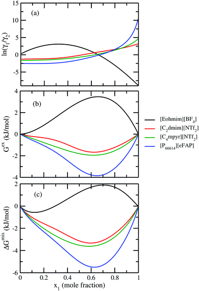
In Fig. 7, we have shown the excess Gibbs energy with varying solute mole fractions for three binary mixtures of CO2 and ionic liquid mixtures showing (1) maximum, (2) medium and (3) least CO2 gas solubility, respectively.
 |
| | Fig. 7 (a) lnγ1/γ2, in figure (b) Gex and, in figure (c) Gmix have been shown as a function of solute mole fraction. | |
In all three cases, we observed that the excess Gibbs energy shows a minimum at mixture compositions other than 50:50 composition of the binary solution and also the free energy curve does not symmetrically decay at the two ends. This asymmetric behavior of the excess free energy vs. x1 plot is in agreement with the asymmetric behavior of the model. To confirm this asymmetric behavior of the solution, we also plot the logarithm of the ratio of the activity coefficients  of solute and solvent species with variation of solute mole fractions xi. The non linear curve shown in Fig. 7 arises due to the asymmetric nature of the solution, otherwise it would be a straight line.1
We also plot the logarithm of activity coefficient with x1 for both the solute and solvent species. The two curves are found to intersect each other at a composition different from the 50:50 mixture composition in Fig. 8. All these results for asymmetric interactions indicate towards the different types of interaction present between the solute and solvent molecules in those vapor–liquid equilibria involving CO2 in ionic liquids.
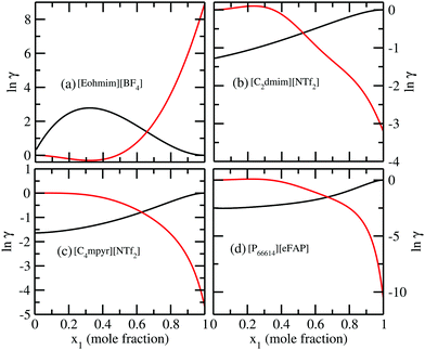 |
| | Fig. 8 (a–d) lnγ vs. solute mole fractions plotted for ILs showing least, medium and high solubility of CO2 gas. The solid black and red curves are for the solute and solvent molecules, respectively. The increasing order of solubility is [Eohmim][BF4] < [C2dmim][NTf2] ∼ [C4mpyr][NTf2] < [P66614][eFAP]. | |
The new model was used to observe the change in Gex and ΔGmix as a function of solute concentration. The ionic liquid showing least CO2 solubility is found to show positive Gex and ΔGmix over some solute concentration with respect to the ionic liquid showing maximum CO2 solubility.
5.3 Solubility of CO2 in RTILs at low partial pressure
In this work, the CO2 solubility in ionic liquid at a low partial pressure (1 bar) of the gas has been calculated. We use our model to calculate the solubility of CO2 in 33 ionic liquids for which experimental data are available for comparison. The experimental results of solubility have been taken from the references stated in the work of Lin et al.31 All the calculations have been done in two phases: (i) the solubility at room temperature (293.15 K to 303.15 K) (Fig. 9) and (ii) the solubility for a wide range of temperatures (283 K to 333.15 K) and at an atmospheric pressure of 1 bar (Fig. 10). Fig. 9 and 10 show a comparison of COSMOSAC-LANL with experimental data and the previous model COSMOSAC-2013. The % errors in the linear regression for COSMOSAC-LANL and COSMOSAC-2013 are 17.2% and 30%, respectively. The percentage error is calculated using the relation  . From Fig. 10, it is also clear that the predictive and accuracy power of the COSMOSAC-LANL model is good to produce the experimental solubility with respect to the COSMOSAC-2013 model.
 |
| | Fig. 9 Solubility of CO2 in different ionic liquids at room temperature (293.15 K to 303.15 K) and at a low partial pressure of 1 bar. | |
 |
| | Fig. 10 Experimental vs. calculated solubility of CO2 in different ionic liquids at varying temperatures (283 K to 333.15 K) and at 1 bar partial pressure. | |
Table 6 shows the results obtained using the COSMOSAC-LANL and COSMOSAC-2013 models for the solubility of CO2 in ionic liquids at room temperature and 1 bar partial pressure. In the case of COSMOSAC-LANL and COSMOSAC-2013 models, calculations on solubility and Henry's constant at room temperature and over a wide range of temperatures have been performed. Accuracy of the model has been tested by calculating the error percentage (average absolute relative deviation (AARD)), 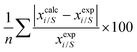
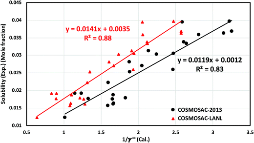
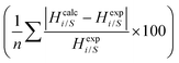 for solubility (Henry's constant). The present model is found to improve the solubility (Henry's constant) with a minimum percentage error of 14% (16.7%) in comparison to the COSMOSAC-2013 model over a wide range of temperatures for 33 ionic liquids (over 79 data points) at 1 bar partial pressure. At room temperature, the percentage of error calculated for solubility (Henry constant) is 13% (14%). The solubility results at room temperature and for a wide range of temperatures have been given in Tables 7 and 8, respectively. From eqn (17), we know that xi = 1/Hi/S(T,P) = 1/(γ∞i/Sfi(T,P)). Therefore, Henry's constant is directly related to the activity coefficient at infinite dilution at a particular temperature. Fig. 11 shows the direct correlation between experimental solubilities and 1/γ∞i/S for both COSMOSAC-LANL and COSMOSAC-2013 models at a particular temperature and at 1 bar partial pressure. A good correlation has been observed using the new COSMOSAC-LANL model (R2 = 0.88). We also calculate the % error in the linear regression for the ideal solvation case when γCO2 = 1 for the two models at an average temperature of 298.15 K and average fugacity of 64.30 bar. The results for COSMOSAC-2013 and COSMOSAC-LANL model are 30% and 10%, respectively. The calculated percentage error in the fugacity is
 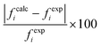 at 298.15 K. The fexpi has been calculated using the relation stated in eqn (19) at a particular temperature. The calculated average absolute relative deviations in the calculated solubilities (Henry's constant) are 12% (13%) for COSMOSAC-LANL and 27% (20%) for the COSMOSAC-2013 model, respectively, at the average room temperature (298.15 K) and at 1 bar partial pressure. The results in the form of the Henry constant have not been shown here, however the results can be obtained from the relation between the solubility and Henry's constant i.e.; xi = 1/Hi at 1 bar partial pressure in the low solubility region used in this study. The result is shown in Table S2 in the ESI.†
Table 7 Solubility of CO2 in 33 ionic liquids at 1 bar partial pressure
| Numbers |
Ionic liquids |
Temperature (K) |
Exp. solubility (mole fraction) |
COSMOSAC-LANL |
COSMOSAC-201324 |
| 1 |
[Eohmim][BF4] |
303.15 |
0.009 |
0.01 |
0.006 |
| 2 |
[C2mim][BF4] |
298 |
0.012 |
0.01 |
0.016 |
| 3 |
[C2mim][DCA] |
303.1 |
0.013 |
0.01 |
0.014 |
| 4 |
[C2mim][EtSO4] |
293.15 |
0.015 |
0.021 |
0.033 |
| 5 |
[C4py][DCA] |
298.15 |
0.016 |
0.017 |
0.025 |
| 6 |
[C4dmim][PF6] |
298.1 |
0.016 |
0.02 |
0.026 |
| 7 |
[C4dmim][BF4] |
298.1 |
0.016 |
0.017 |
0.026 |
| 8 |
[C4py][F3Ac] |
298.15 |
0.018 |
0.02 |
0.018 |
| 9 |
[C4mim][BF4] |
298.1 |
0.018 |
0.014 |
0.021 |
| 10 |
[C4mim][DCA] |
298 |
0.018 |
0.019 |
0.028 |
| 11 |
[C8mim][BF4] |
303 |
0.019 |
0.021 |
0.028 |
| 12 |
[C4mim][PF6] |
298.1 |
0.019 |
0.015 |
0.015 |
| 13 |
[C2mim][OTf] |
298.2 |
0.019 |
0.014 |
0.019 |
| 14 |
[C3mim][PF6] |
298.1 |
0.019 |
0.013 |
0.018 |
| 15 |
[C4mim][OTf] |
298.15 |
0.022 |
0.02 |
0.018 |
| 16 |
[C6tma][NTf2] |
303.15 |
0.023 |
0.022 |
0.044 |
| 17 |
[C2dmim][NTf2] |
298.1 |
0.025 |
0.021 |
0.029 |
| 18 |
[C4mpyr][NTf2] |
298.15 |
0.026 |
0.029 |
0.038 |
| 19 |
[C3mim]NTf2] |
298.1 |
0.027 |
0.026 |
0.032 |
| 20 |
[C2mim][NTf2] |
298.1 |
0.028 |
0.024 |
0.029 |
| 21 |
[C4mim][NTf2] |
298.1 |
0.03 |
0.027 |
0.035 |
| 22 |
[C6mpy][NTf2] |
298 |
0.03 |
0.03 |
0.039 |
| 23 |
[C4py][NTf2] |
298.15 |
0.031 |
0.03 |
0.033 |
| 24 |
[C10mim][NTf2] |
303.4 |
0.033 |
0.032 |
0.04 |
| 25 |
[C8mim][NTf2] |
298.1 |
0.033 |
0.033 |
0.041 |
| 26 |
[C6mim][NTf2] |
298.06 |
0.034 |
0.033 |
0.041 |
| 27 |
[C8py][NTf2] |
298.15 |
0.036 |
0.032 |
0.044 |
| 28 |
[C10py][NTf2] |
298.15 |
0.036 |
0.04 |
0.049 |
| 29 |
[C12py][NTf2] |
298.15 |
0.037 |
0.04 |
0.051 |
| 30 |
[C1c4pyrro][eFAP] |
303.16 |
0.039 |
0.03 |
0.039 |
| 31 |
[C8h4f13][NTf2] |
298.04 |
0.04 |
0.032 |
0.04 |
| 32 |
[C6mim][eFAP] |
298.6 |
0.04 |
0.038 |
0.05 |
| 33 |
[P66614][eFAP] |
303.19 |
0.052 |
0.062 |
0.07 |
|
|
| — |
AARD (%) |
— |
— |
13 |
30 |
Table 8 Solubility of CO2 in 33 ionic liquids at 1 bar partial pressure
| Numbers |
Ionic liquids |
Temperature (K) |
Exp. solubility (mole fraction) |
COSMOSAC-LANL |
COSMOSAC-2013 |
| 1 |
[C2mim][OTf] |
298.2 |
0.019 |
0.014 |
0.019 |
| 2 |
|
303.1 |
0.014 |
0.012 |
0.017 |
| 3 |
[C2mim][DCA] |
303.1 |
0.013 |
0.01 |
0.014 |
| 4 |
[C2mim][BF4] |
298 |
0.012 |
0.01 |
0.016 |
| 5 |
|
313 |
0.01 |
0.007 |
0.011 |
| 6 |
[C2mim][NTf2] |
283.1 |
0.04 |
0.033 |
0.041 |
| 7 |
|
298.1 |
0.028 |
0.024 |
0.029 |
| 8 |
|
303.45 |
0.025 |
0.021 |
0.026 |
| 9 |
|
313 |
0.02 |
0.017 |
0.021 |
| 10 |
[C2mim][EtSO4] |
293.15 |
0.015 |
0.021 |
0.033 |
| 11 |
[C2dmim][NTf2] |
283.1 |
0.035 |
0.03 |
0.042 |
| 12 |
|
298.1 |
0.025 |
0.021 |
0.029 |
| 13 |
[C3mim][PF6] |
298.1 |
0.019 |
0.013 |
0.018 |
| 14 |
[C3mim]NTf2] |
298.1 |
0.027 |
0.026 |
0.032 |
| 15 |
[C4mim][BF4] |
283.1 |
0.025 |
0.021 |
0.03 |
| 16 |
|
298.1 |
0.018 |
0.014 |
0.021 |
| 17 |
|
303.38 |
0.016 |
0.013 |
0.018 |
| 18 |
|
313 |
0.013 |
0.01 |
0.015 |
| 19 |
[C4mim][NTf2] |
283.15 |
0.04 |
0.042 |
0.049 |
| 20 |
|
298.1 |
0.03 |
0.027 |
0.035 |
| 21 |
|
303 |
0.03 |
0.024 |
0.031 |
| 22 |
[C4mim][PF6] |
283.1 |
0.026 |
0.022 |
0.037 |
| 23 |
|
293.17 |
0.021 |
0.017 |
0.029 |
| 24 |
|
298.1 |
0.019 |
0.015 |
0.021 |
| 25 |
|
303 |
0.017 |
0.014 |
0.023 |
| 26 |
[C4mim][DCA] |
294 |
0.019 |
0.021 |
0.031 |
| 27 |
|
298 |
0.018 |
0.019 |
0.028 |
| 28 |
|
303 |
0.016 |
0.017 |
0.025 |
| 29 |
|
313 |
0.013 |
0.013 |
0.02 |
| 30 |
|
323 |
0.011 |
0.011 |
0.016 |
| 31 |
[C4mim][OTf] |
298.15 |
0.022 |
0.018 |
0.025 |
| 32 |
[C4dmim][PF6] |
283.1 |
0.021 |
0.028 |
0.037 |
| 33 |
|
298.1 |
0.016 |
0.02 |
0.026 |
| 34 |
[C4dmim][BF4] |
283.1 |
0.022 |
0.025 |
0.038 |
| 35 |
|
298.1 |
0.016 |
0.017 |
0.026 |
| 36 |
[C6mim][eFAP] |
298.6 |
0.04 |
0.038 |
0.05 |
| 37 |
[C6mim][NTf2] |
288.48 |
0.041 |
0.042 |
0.051 |
| 38 |
|
293.21 |
0.037 |
0.037 |
0.045 |
| 39 |
|
298.06 |
0.034 |
0.033 |
0.041 |
| 40 |
[C6mim][NTf2] |
303.44 |
0.03 |
0.03 |
0.036 |
| 41 |
|
313 |
0.024 |
0.024 |
0.03 |
| 42 |
[C8mim][NTf2] |
298.1 |
0.033 |
0.033 |
0.041 |
| 43 |
|
303.03 |
0.03 |
0.03 |
0.037 |
| 44 |
|
313.02 |
0.026 |
0.024 |
0.03 |
| 45 |
[C8mim][BF4] |
303 |
0.019 |
0.021 |
0.028 |
| 46 |
[C10mim][NTf2] |
303.4 |
0.033 |
0.032 |
0.04 |
| 47 |
|
313.15 |
0.028 |
0.026 |
0.033 |
| 48 |
|
313.2 |
0.027 |
0.026 |
0.033 |
| 49 |
|
323.1 |
0.023 |
0.021 |
0.027 |
| 50 |
[C4mpyr][NTf2] |
283.15 |
0.033 |
0.042 |
0.055 |
| 51 |
|
298.15 |
0.026 |
0.029 |
0.038 |
| 52 |
[C1c4pyrro][eFAP] |
303.16 |
0.039 |
0.03 |
0.039 |
| 53 |
|
303.18 |
0.039 |
0.03 |
0.039 |
| 54 |
|
313.15 |
0.033 |
0.023 |
0.031 |
| 55 |
|
313.19 |
0.033 |
0.023 |
0.031 |
| 56 |
|
313.22 |
0.033 |
0.023 |
0.031 |
| 57 |
|
323.12 |
0.029 |
0.02 |
0.026 |
| 58 |
|
323.22 |
0.028 |
0.02 |
0.025 |
| 59 |
[P66614][eFAP] |
303.19 |
0.052 |
0.062 |
0.07 |
| 60 |
|
313.19 |
0.046 |
0.05 |
0.057 |
| 61 |
|
313.25 |
0.046 |
0.05 |
0.056 |
| 62 |
|
323.23 |
0.041 |
0.041 |
0.046 |
| 63 |
[C6mpy][NTf2] |
283 |
0.039 |
0.039 |
0.055 |
| 64 |
|
298 |
0.03 |
0.03 |
0.039 |
| 65 |
[C6tma][NTf2] |
303.15 |
0.023 |
0.022 |
0.044 |
| 66 |
[C4py][F3Ac] |
298.15 |
0.018 |
0.018 |
0.026 |
| 67 |
[C4py][DCA] |
298.15 |
0.016 |
0.017 |
0.025 |
| 68 |
[C4py][NTf2] |
298.15 |
0.031 |
0.03 |
0.033 |
| 69 |
|
313.15 |
0.025 |
0.02 |
0.024 |
| 70 |
|
333.15 |
0.019 |
0.013 |
0.016 |
| 71 |
[C8py][NTf2] |
298.15 |
0.036 |
0.032 |
0.044 |
| 72 |
|
313.15 |
0.028 |
0.023 |
0.032 |
| 73 |
|
333.15 |
0.024 |
0.016 |
0.021 |
| 74 |
[C10py][NTf2] |
298.15 |
0.036 |
0.04 |
0.049 |
| 75 |
[C12py][NTf2] |
298.15 |
0.037 |
0.04 |
0.051 |
| 76 |
|
313.15 |
0.028 |
0.029 |
0.037 |
| 77 |
|
333.15 |
0.029 |
0.02 |
0.025 |
| 78 |
[Eohmim][BF4] |
303.15 |
0.009 |
1.00 × 10−02 |
0.006 |
| 79 |
[C8h4f13][NTf2] |
298.04 |
0.04 |
0.032 |
0.04 |
|
|
| — |
AARD (%) |
— |
— |
14 |
26 |
 |
| | Fig. 11 Experimental solubility of CO2 in different ionic liquids as a function of (1/γ∞i/S) at 298.15 K at 1 bar partial pressure. | |
Except for [C2mim][OTf], [C3mim][PF6], [C1C4pyrro][eFAP] and [C8h4f13][NTf2] ionic liquids, for the rest of the ionic liquids improved solubility results were obtained using the COSMOSAC-LANL activity coefficient model. The possible reason for the deviation in those cases is the combinatorial interaction present in the model. For those four ionic liquids, the results obtained using the COSMOSAC-2013 model are in good agreement with the experimental results. We found that the model can be modified for those four ionic liquids by considering only 3-suffix Margules expression without any SG term present in the model for the asymmetric interaction according to the data in Table 2. We observed that the calculated solubility at room temperature and at 1 bar partial pressure is found to improve to 11% for 29 from 13% for 33 selected ionic liquids. The AARD for solubility is improved to 13% for 29 from 14% for 33 selected ionic liquids for a wide range of temperatures and at 1 bar partial pressure.
5.4 Ideal-dilute selectivity of CO2 over CH4
The study of absorption selectivity between the CO2 over the CH4 gas is important to large scale industries such as the natural gas sweetening process involving the selectivity between CO2 and CH4.31,42 We used our model for calculating the selectivity of CO2/CH4 for which the experimental data are available for comparison at a low partial pressure of 1 bar. The selectivity has been calculated from the single solubility data of a gas and thus by taking the ratio of that solubility data, i.e.;  . The experimental and calculated results are given in Table 9. All the experimental results on selectivity have been taken from the references stated in the work of Lin et al.31 The present method is found to predict the selectivity between CO2 and CH4 within 12% error at a low partial pressure of 1 bar and in the low solubility region.
Table 9 Selectivity between CO2 and CH4 gases at 1 bar partial pressure
| Numbers |
Ionic liquids |
Temperature (K) |
x
CO2/xCH4 (exp.)31 |
COSMOSAC-LANL |
| 1 |
[C2mim][OTf] |
303.15 |
19 |
18.04 |
| 2 |
|
313 |
17 |
16.05 |
| 3 |
[C2mim][DCA] |
303.15 |
23 |
21.25 |
| 4 |
|
313 |
21 |
21.32 |
| 5 |
[C2mim][NTf2] |
298.15 |
15 |
12.59 |
| 6 |
|
303.15 |
12 |
12.55 |
| 7 |
|
313.15 |
12 |
12.64 |
| 8 |
[C4mim][NTf2] |
298 |
12 |
11.07 |
| 9 |
[C6mim][NTf2] |
298.15 |
10 |
10.59 |
| 10 |
|
303.15 |
9 |
9.16 |
| 11 |
|
313.15 |
8 |
10.8 |
| 12 |
[C8mim][NTf2] |
298 |
9 |
10.37 |
| 13 |
[C4mim][PF6] |
303.15 |
13 |
12.9 |
| 14 |
[C2mim][BF4] |
303.15 |
22 |
25.18 |
| 15 |
|
313.15 |
20 |
22.34 |
| 16 |
[C4mim][BF4] |
303.15 |
13 |
16.93 |
| 17 |
[C1oc2mim][NTf2] |
313.15 |
13 |
12.34 |
| 18 |
[C1mim][MeSO4] |
313.15 |
18 |
10 |
|
|
| — |
AARD (%) |
— |
— |
12 |
5.5 Screening of ionic liquids based on the solvophobic property
We proposed a new method to screen ionic liquids for the best solubility of CO2 gas capture based on the solvophobic effect of the ionic liquids reported in the work of Sedov et al.43 Solvophobic effect is the generalized concept of hydrophobic effect for self associating ionic liquids and the key driving force of self-assembly of amphiphilic compounds into the mesophase structures such as micelles, vesicles, bilayers, microemulsions and emulsions.44 Similar to the recent work of Sedov et al.43 in 2016, we define the solvophobic effect in this work. In ionic liquids, the concentration of ions (the cation plus the anion of the liquids), Ci = 1/Vm, which is the inverse of molar volume of the ionic liquid, is correlated with thermodynamic solvation properties (ΔGsolv). Since the Henry constant and free energy of solvation are related to each other following the thermodynamic relation given in eqn (18), the experimental free energy of solvation of CO2 for all ionic liquids has been calculated and correlated to the inverse of the molar volume of the ionic liquids in Fig. 12. We have also shown the correlation between the experimental solubility and the inverse of the molar volume in Fig. 13. A correlation between the calculated and the experimental free energy of solvation has been shown in Fig. S6 in the ESI.† The calculated free energy of solvation has been obtained using the both COSMOSAC model in this study. The % error in the linear regression is 0.43% in the COSMOSAC-LANL model and 21.45% in COSMOSAC-2013 (the result is shown Fig. S6, ESI†) for free energy solvation. The molar volume has been calculated using the following equation Vm (cm3 mol−1) = VCOSMO (Å3 per molecule) × (10−24 cm3 Å−3) × 6.02 × 1023 molecules per mol. The calculated COSMO volume, temperature, experimental solubility and experimental free energy of solvation have been given in Table 10 separately.
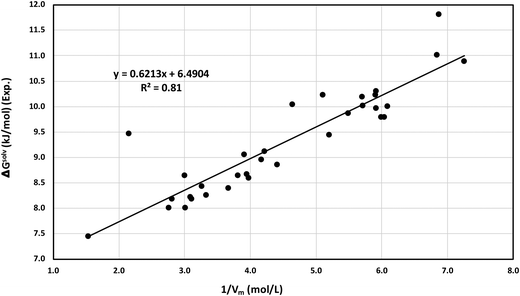 |
| | Fig. 12 Correlation between the experimental solvation free energy and calculated 1/Vm under ambient conditions. | |
 |
| | Fig. 13 Correlation between the experimental solubility and calculated 1/Vm under ambient conditions. | |
Table 10 COSMO volume, solubility and free energy of solvation at 1 bar partial pressure
| Numbers |
Ionic liquids |
Temperature (K) |
COSMO volume |
V
m
|
1/Vm |
Exp. H (bar) |
Solubility |
ΔGsolv (kJ mol−1) |
| 1 |
[Eohmim][BF4] |
303.15 |
241.79 |
145.56 |
6.87 |
108.35 |
0.009 |
11.81 |
| 2 |
[C2mim][BF4] |
298 |
228.86 |
137.77 |
7.26 |
81.06 |
0.012 |
10.89 |
| 3 |
[C2mim][DCA] |
303.1 |
242.95 |
146.26 |
6.84 |
79.03 |
0.013 |
11.01 |
| 4 |
[C2mim][EtSO4] |
293.15 |
281.10 |
169.22 |
5.91 |
66.5 |
0.015 |
10.23 |
| 5 |
[C4py][DCA] |
298.15 |
280.79 |
169.03 |
5.92 |
63.9 |
0.016 |
10.30 |
| 6 |
[C4dmim][PF6] |
298.1 |
325.66 |
196.05 |
5.10 |
61.8 |
0.016 |
10.22 |
| 7 |
[C4dmim][BF4] |
298.1 |
291.55 |
175.51 |
5.70 |
61 |
0.016 |
10.19 |
| 8 |
[C4py][F3Ac] |
298.15 |
290.83 |
175.08 |
5.71 |
56.9 |
0.018 |
10.02 |
| 9 |
[C4mim][BF4] |
298.1 |
272.74 |
164.19 |
6.09 |
56.5 |
0.018 |
10.00 |
| 10 |
[C4mim][DCA] |
298 |
281.05 |
169.19 |
5.91 |
55.9 |
0.018 |
9.97 |
| 11 |
[C8mim][BF4] |
303 |
358.01 |
215.52 |
4.64 |
53.9 |
0.019 |
10.04 |
| 12 |
[C4mim][PF6] |
298.1 |
302.79 |
182.28 |
5.49 |
53.4 |
0.019 |
9.86 |
| 13 |
[C2mim][OTf] |
298.2 |
275.19 |
165.66 |
6.04 |
52 |
0.019 |
9.80 |
| 14 |
[C3mim][PF6] |
298.1 |
277.22 |
166.89 |
5.99 |
52 |
0.019 |
9.79 |
| 15 |
[C4mim][OTf] |
298.15 |
319.42 |
192.29 |
5.20 |
45 |
0.022 |
9.44 |
| 16 |
[C6tma][NTf2] |
303.15 |
772.41 |
464.99 |
2.15 |
42.66 |
0.023 |
9.46 |
| 17 |
[C2dmim][NTf2] |
298.1 |
393.78 |
237.06 |
4.22 |
39.6 |
0.025 |
9.12 |
| 18 |
[C4mpyr][NTf2] |
298.15 |
425.40 |
256.09 |
3.90 |
38.6 |
0.026 |
9.06 |
| 19 |
[C3mim]NTf2] |
298.1 |
398.02 |
239.61 |
4.17 |
37 |
0.027 |
8.95 |
| 20 |
[C2mim][NTf2] |
298.1 |
376.49 |
226.65 |
4.41 |
35.6 |
0.028 |
8.85 |
| 21 |
[C4mim][NTf2] |
298.1 |
421.39 |
253.68 |
3.94 |
33 |
0.030 |
8.67 |
| 22 |
[C6mpy][NTf2] |
298 |
435.46 |
262.14 |
3.81 |
32.8 |
0.030 |
8.65 |
| 23 |
[C4py][NTf2] |
298.15 |
417.75 |
251.49 |
3.98 |
32 |
0.031 |
8.59 |
| 24 |
[C10mim][NTf2] |
303.4 |
554.22 |
333.64 |
3.00 |
30.75 |
0.033 |
8.64 |
| 25 |
[C8mim][NTf2] |
298.1 |
509.04 |
306.44 |
3.26 |
30 |
0.033 |
8.43 |
| 26 |
[C6mim][NTf2] |
298.06 |
452.71 |
272.53 |
3.67 |
29.54 |
0.034 |
8.39 |
| 27 |
[C8py][NTf2] |
298.15 |
499.21 |
300.52 |
3.33 |
27.9 |
0.036 |
8.25 |
| 28 |
[C10py][NTf2] |
298.15 |
538.25 |
324.03 |
3.09 |
27.5 |
0.036 |
8.21 |
| 29 |
[C12py][NTf2] |
298.15 |
590.78 |
355.65 |
2.81 |
27.1 |
0.037 |
8.18 |
| 30 |
[C1c4pyrro][eFAP] |
303.16 |
534.64 |
321.86 |
3.11 |
25.7 |
0.039 |
8.18 |
| 31 |
[C8h4f13][NTf2] |
298.04 |
601.20 |
361.92 |
2.76 |
25.3 |
0.040 |
8.01 |
| 32 |
[C6mim][eFAP] |
298.6 |
551.90 |
332.24 |
3.01 |
25.2 |
0.040 |
8.01 |
| 33 |
[P66614][eFAP] |
303.19 |
1083.02 |
651.98 |
1.53 |
19.2 |
0.052 |
7.45 |
We compared the experimental ΔGsolv (exp.) vs. 1/Vm (exp.) and ΔGsolv (exp.) vs. 1/Vm (cal.) for 16 different room temperature ionic liquids for which the experimental densities were available under ambient conditions. We also plotted 1/Vm (exp.) vs. 1/Vm (cal.) and calculated the AARD. The results are given in Fig. S7(a, b) and Table S3 in the ESI.† We found that the COSMOSAC model underestimates the 1/Vm (cal.) by 14.1%. The plot shown in Fig. S7(b) in the ESI,† indicates small improvement in the results of the inverse of experimental and calculated molar volume. The model shows significant improvement when we compared the experimental and the calculated ΔGsolv obtained from both the COSMOSAC-2013 and COSMOSAC-LANL models. The result is shown in Fig. S6 (ESI†). The COSMOSAC-LANL model predicts the free energy of solvation within 4% error while the COSMOSAC-2013 model predicts it within 7% error. Also the correlation between the experimental and the calculated free energy of solvation improves for the COSMOSAC-LANL model (R2 = 0.87) almost by 10% with respect to the COSMOSAC-2013 model (R2 = 0.78). The molar volume has been calculated using the scheme mentioned in the link of COSMO-RS tutorial available in SCM (https://www.scm.com/doc/Tutorials/COSMO-RS) for ionic liquids,32 however we made a little change in our calculation for single molecule treatment of the ionic liquid. The molecular weight and density of 16 different ionic liquids has been taken from the IL Thermo database.45
We have screened the ionic liquids for CO2 gas for the ionic liquids mainly containing [NTf2]− anion, [C2mim]+ and [C4mim]+ cations for which the experimental solubility data were available. We observed that these are the few common cations and anions usually used for CO2 gas capture using ionic liquids. A relationship has been established between the inverse of the calculated molar volume (1/Vm) (x) obtained from the quantum COSMO calculations and the experimental solubility data (y) for each case. A correlation has been observed between these two properties for all the ions and results are given in ESI,† in Fig. S8–S10. The linear relationships to screen the cations (mainly imidazolium and pyrrolinidium) against a [NTf2]− anion is y = −0.007x + 0.0571 with R2 = 0.77. The same to screen the different anions for [C4mim]+ and [C2mim]+ cations are y = −0.0062x + 0.0541 for R2 = 0.96 and y = −0.0057x + 0.052 for R2 = 0.90, respectively. Therefore, one will be able to compute the solubility of an unknown ionic liquid having these cation or anion common in them using these relations, provided the molar volume is calculated using quantum COSMO calculation within the ADF-COSMOSAC-2013 model implemented in ADF-2016 software. Also one can predict the solubility of CO2 gas in any ionic liquid very well according to the relation (y = −0.0062x + 0.0536 with R2 = 0.82) shown in Fig. 13. We observe that the outlier present in the Fig. 13 is the [C6tma][NTf2] ionic liquid which is a dication dianion ionic liquid. The coefficient of determination is improved by 10% (R2 = 0.92; result is not shown here) when we assume the molar volume/cation–anion pair present in such type of ionic liquid.
6 Conclusion
A new thermodynamic model is presented to express the solution properties for CO2 and CH4 in room temperature ionic liquids (RTILs) under varying thermodynamic conditions. The new thermodynamic model is composed of the Staverman–Guggenheim (SG) term due to the long-range interaction and short range asymmetric interaction (3-suffix Margules function) between the solute and solvent species in a solution. For the short range asymmetric interaction, we chose the 3-suffix Margules function for the asymmetric solution because we assume that the long range combinatorial term will be responsible for the entropy driven solubility phenomenon due to the size and shape differences between the solute and solvent species. We have shown in this study that the new thermodynamic model for activity coefficient improves the solubility prediction of CO2 in ionic liquids when it was used with the ADF-COSMOSAC-2013 model. We calculated the solubility from the Henry constant available from the fugacity and activity coefficient at infinite dilution for the two greenhouse gases mainly CO2 and CH4 in RTILs. We take 33 such example cases to test our model which is comprised of a long range combinatorial term along with the short range asymmetric interaction. Our present model was not only able to improve the quantitative prediction of solubility of CO2 in those 33 ionic liquids, but was also able to explain other thermodynamical and physical properties of those systems. It has been found from our study that the present model improves the solubility of CO2 gas by 17% with respect to the COSMOSAC-2013 model at room temperature over 33 points. For the quantitive prediction of Henry's constant, the calculated percentage of errors is (1) 14% for COSMOSAC-LANL and (2) 22% for COSMOSAC-2013 at room temperature over 33 points, respectively. For a wide range of temperatures, the present model predicts solubility within 14% AARD with respect to the COSMOSAC-2013 model over 79 points used in this study. With this new model the selectivity between CO2/CH4 was predicted within 12% error over 18 points. We have proposed a new scheme to screen ionic liquids for the best CO2 solubility using the concept of solvophobic effect which is a correlation between the solubility and the inverse of the molar volume of the ionic liquid resulting from the first principles calculation in this model in addition to the conventional screening method which is a correlation between the solubility and the 1/γ∞i/S at a particular temperature. Using the new COSMOSAC-LANL thermodynamic model the solvation mechanism of CO2 and CH4 in those ionic liquids has been explained. The calculated theoretical results are found to be in good agreement with the other experimental and theoretical results where they were available. The only drawback of this model is that it cannot be applied to model the systems tending towards the supercritical condition because the present model within the COSMO-RS frame work cannot handle the free volume effect and therefore the vapor–liquid transition.46 However, the model can be applied to a certain range of pressures and temperatures for both CO2 and CH4 gases to predict their solubility in ionic liquids.
The new thermodynamic model can be applied to study the other vapor–liquid, liquid–liquid and solid–liquid equilibria. Very recently, the new COSMOSAC-LANL model has been applied to predict the solubility of metal complexes in ionic liquids to screen the metal complexes25 and ionic liquids for the best solubility of the redox active species in ionic liquids. The solvation mechanism of those systems has been explained using the new COSMOSAC-LANL model.
Conflicts of interest
There are no conflicts to declare.
Appendix A
At infinite dilute, when x1 → 0 and x2 → 1, eqn (6) will be reduced to  for solute species (1). Now after adding and substituting the value of (α1 + β1) in the expression of lnγ∞1, one will get
 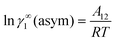 and hence,
| | | A12 = RTlnγ∞1(asym). | (23) |
Similarly, when x2 → 0 and x1 → 1, eqn (7) will be reduced to  for solvent species (2). Now after adding and substituting the value of (α2 + β2) in the expression of lnγ∞2, one will get
  for the solvent species (2) and therefore,
| | | A21 = RTlnγ∞2(asym). | (24) |
Hence, at infinite dilution, one can calculate Margules parameters from the activity coefficients at infinite dilution from the above two equations. Since, in this article the Margules parameters are obtained from the activity coefficient at infinite dilution calculated using the COSMOSAC-2013 model, therefore one can write
| |  | (25) |
and
| |  | (26) |
Substituting the value of A12 and A21 in eqn (23) and (24), one will get
| | | lnγ∞1(asym) = lnγ∞1(COSMOSAC), | (27) |
and
| | | lnγ∞2(asym) = lnγ∞2(COSMOSAC). | (28) |
Table 2 shows the values of activity coefficients at infinite dilution calculated from the asymmetric term and the ADF-COSMOSAC-2013 model.
Since we know that
| | | lnγi/S(COSMOSAC-2013) = lnγi/S(res) + lnγi/S(comb) + lnγi/S(dis), | (29) |
therefore,
| | | lnγi/S(asym) = lnγi/S(res) + lnγi/S(comb) + lnγi/S(dis). | (30) |
Now, our asymmetric model is
| | | lnγi/S(COSMOSAC-LANL) = lnγi/S(comb) + lnγi/S(asym). | (31) |
Substituting lnγi/S(asym) in the above equation, one will get
| | | lnγi/S(COSMOSAC-LANL) = 2lnγi/S(comb) + lnγi/S(dis) + lnγi/S(res). | (32) |
Therefore, subtracting eqn (29) from eqn (32), one will get the relationship between the two models which is valid at infinite dilution and that is
| | | lnγi/S(COSMOSAC-LANL) − lnγi/S(COSMOSAC-2013) = lnγi/S(comb). | (33) |
Appendix B
At infinite dilution (x1 → 0 and x2 → 1), we have defined the lnγcompute1 and lnγmodel1 for the solute particle in the following way| | | lnγcompute1 = lnγcompute1(comb) + lnγcompute1(asym), | (34) |
and| | | lnγmodel1 = lnγmodel1(comb) + lnγmodel1(asym). | (35) |
Since we did not change the term due to combinatorial contribution, lnγcompute1(comb) = lnγ1model(comb).
Subtracting eqn (35) from eqn (34), one will get
| | 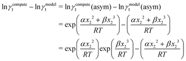 | (36) |
Now, one can write the above expression using the Taylor series expansion when x2 → 0;
| | 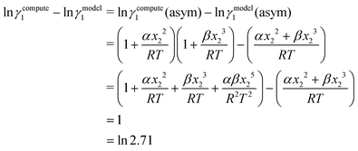 | (37) |
Now, simplifying the above equation, one will get for species 1, when x2 → 0;
| |  | (38) |
Similarly, one can derive the same for species 2, when x1 → 0 i.e.;
| | 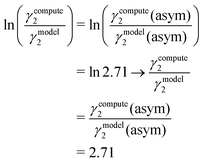 | (39) |
Therefore,
| | | lnγ1/2(real) = lnγ1/2(compute) = 1 + lnγ1/2(model). | (40) |
This relation holds when the system is in the region x2or1 → 0. Since the above equation is valid when the binary system approaches x1/2 → 1, x2/1 → 0 for a species, so one will correct the calculated activity coefficient at infinite dilution (x1/2 → 0, x2/1 → 1) using the following relation
| | | lnγ1/2(real) = lnγ1/2(compute) = 1 + lnγ1/2(model), | (41) |
for which the minimum computed asymmetric interaction is less than 1 according to Appendix C.
Appendix C
The minimum criteria for when to use eqn (9) and when to use eqn (12) for the calculation of the activity coefficient at infinite dilution have been explained. One can write eqn (14) as| | 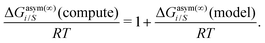 | (42) |
We already know from eqn (4)| |  | (43) |
Now we can also define,| | 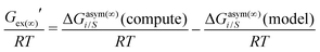 | (44) |
Now, to be, 
| |  | (45) |
because according to the model,| | 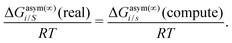 | (46) |
Now substituting eqn (45) in eqn (42), one will get,
| |  | (47) |
and thus
| | | lnγasym(∞)i/S(compute) = 1. | (48) |
Therefore, the minimum computed asymmetric interaction (lnγasym(∞)i/S(compute)) should be of the order of 1 stated according to Appendix C to apply the model stated in eqn (9) over the model stated in eqn (12).
Acknowledgements
This work has been funded by the “Laboratory Directed Research and Development” program grant no. 20170046DR in Los Alamos National Laboratory, USA. Los Alamos National Laboratory is operated by Triad National Security under contract number 89233218CNA000001 for the Department of Energy.
References
-
J. M. Prausnitz, R. N. Lichtenthaler and E. G. de Azevedo, Molecular Thermodynamics of Fluid Phase Equilibria, Prentice Hall, New York, 3rd edn, 1999 Search PubMed.
-
S. I. Sandler, Chemical, Biochemical, and Engineering Thermodynamics, John Wiley & Sons, Inc., New York, 4th edn, 2005 Search PubMed.
- W. Cao, A. Fredenslund and P. Rasmussen, Ind. Eng. Chem. Res., 1992, 31, 2603–2619 CrossRef CAS.
- W. Cao, K. Knudsen, A. Fredenslund and P. Rasmussen, Ind. Eng. Chem. Res., 1993, 32, 2077–2087 CrossRef CAS.
- D. S. Abrams and J. M. Prausnitz, AIChE J., 1975, 21(1), 116–128 CrossRef CAS.
- A. Fredenslund, J. Gmehling and P. Rasmussen, AIChE J., 1975, 21, 1086 CrossRef CAS.
- H. Renon and J. M. Prausnitz, AIChE J., 1968, 14, 135–144 CrossRef CAS.
- J. S. Andreu and L. F. Vega, J. Phys. Chem. C, 2007, 111, 16028–16034 CrossRef CAS.
- J. S. Andreu and L. F. Vega, J. Phys. Chem. B, 2008, 112, 15398–15406 CrossRef CAS PubMed.
- E. K. Karakatsani, I. G. Economou, M. C. Kroon, M. D. Bermejo, C. J. Peters and G.-J. Witkamp, Phys. Chem. Chem. Phys., 2008, 10, 6160–6168 RSC.
- M. C. Kroon, E. K. Karakatsani, I. G. Economou, G.-J. Witkamp and C. J. Peters, J. Phys. Chem. B, 2006, 110, 9262–9269 CrossRef CAS PubMed.
- J. Kumelan, A. P.-S. Kamps, D. Tuma, A. Yokozeki, M. B. Shiflett and G. Maurer, J. Phys. Chem. B, 2008, 112, 3040–3047 CrossRef CAS PubMed.
- R. Kato and J. Gmehling, J. Chem. Thermodyn., 2005, 37, 603–619 CrossRef CAS.
- J. Wang, W. Sun, C. Li and Z. Wang, Fluid Phase Equilib., 2008, 264, 235–241 CrossRef CAS.
- S. Nebig, R. Bölts and J. Gmehling, Fluid Phase Equilib., 2007, 258, 168–178 CrossRef CAS.
- A. Klamt and F. Eckert, Fluid Phase Equilib., 2000, 172, 43–72 CrossRef CAS.
- A. Klamt, Wiley Interdiscip. Rev.: Comput. Mol. Sci., 2011, 1, 699–709 CAS.
- S.-T. Lin and S. I. Sandler, Ind. Eng. Chem. Res., 2002, 41, 899–913 CrossRef CAS.
- A. Klamt and G. Schüürmann, J. Chem. Soc., Perkin Trans. 2, 1993, 799–805 RSC.
- N. A. Gokcen, J. Phase Equilib., 1996, 17, 50–51 CrossRef CAS.
- J. Wisniak, Chem. Eng. Sci., 1983, 38, 969 CrossRef CAS.
- A. J. Staverman, Recl. Trav. Chim. Pay-Bas-J. R. Neth. Chem. Soc., 1950, 69, 163–174 CrossRef CAS.
-
E. A. Guggenheim, Mixtures: The theory of the equilibrium properties of some simple classes of mixtures, solutions and alloys, Clarendon Press, Oxford, UK, 1952 Search PubMed.
- R. Xiong, S. I. Sandler and R. I. Burnett, Ind. Eng. Chem. Res., 2014, 53, 8265–8278 CrossRef CAS.
- A. Karmakar, R. Mukundan, P. Yang and E. R. Batista, RSC Adv., 2019, 9, 18506–18526 RSC.
- A. Klamt, G. J. P. Krooshof and R. Taylor, AIChE J., 2002, 48(10), 2332–2349 CrossRef CAS.
-
A. Klamt, COSMO-RS: From Quantum Chemistry to Fluid Phase Thermodynamics and Drug Design, 1st edn, Elsevier Science, 2005 Search PubMed.
-
P. Atkins and J. de Paula, Physical Chemistry, Oxford University Press, 9th edn, 2010 Search PubMed.
-
R. I. Burnett, Predicting Liquid-Phase Thermodynamic Properties Using COSMO-SAC, University of Delaware, 2012 Search PubMed.
-
J. M. Smith, H. C. V. Ness and M. M. Abott, Introduction to Chemical Engineering Thermodynamics, McGraw-Hill, New York, 2005 Search PubMed.
- B.-S. Lee and S.-T. Lin, Chem. Eng. Sci., 2015, 121, 157–168 CrossRef CAS.
- ADF2016, SCM, Theoretical Chemistry, Vrije Universiteit, Amsterdam, The Netherlands, https://www.scm.com, Software for Chemistry & Materials, 2016.
- O. Hollóczki, F. Malberg, T. Welton and B. Kirchner, Phys. Chem. Chem. Phys., 2014, 16, 16880–16890 RSC.
- B. Kirchner, F. Malberg, D. S. Firaha and O. Hollóczki, J. Phys.: Condens. Matter, 2015, 27, 463002 CrossRef PubMed.
- A. Klamt, V. Jonas, T. Bürgar and J. C. W. Lohrenz, J. Phys. Chem. A, 1998, 102, 5074–5085 CrossRef CAS.
-
A. Kazakov, J. W. Magee, R. D. Chirico, V. Dicky, C. D. Muzny, K. Kroenlein and M. Frenkel, NIST Standard ReferenceDatabase 147: NIST Ionic LiquidsDatabase-(ILThermo). Version 2.0, National Institute of Standards and Technology, Gaithersburg, MD, 2013, p. 20899 Search PubMed.
- S. Stevanovic and M. F. C. Gomes, J. Chem. Thermodyn., 2013, 65–71 CrossRef CAS.
- C.-M. Hsieh, S. I. Sandler and S. T. Lin, Fluid Phase Equilib., 2010, 297, 90–97 CrossRef CAS.
- M. Klähn and A. Seduraman, J. Phys. Chem. B, 2015, 119(31), 10066–10078 CrossRef PubMed.
- C. A. Daly, T. Brinzer, C. Allison, S. Garrett-Roe and S. A. Corcelli, J. Phys. Chem. Lett., 2018, 9(6), 1393–1397 CrossRef CAS PubMed.
- U. Kapoor and J. K. Shah, J. Phys. Chem. B, 2018, 122(42), 9763–9774 CrossRef CAS PubMed.
- M. Ramdin, T. W. de Loos and T. J. Vlugt, Ind. Eng. Chem. Res., 2012, 51, 8149–8177 CrossRef CAS.
- I. A. Sedov and B. N. Solomonov, Fluid Phase Equilib., 2016, 425, 9–14 CrossRef CAS.
- T. L. Greaves and C. J. Drummond, Chem. Soc. Rev., 2008, 37, 1709–1726 RSC.
- Q. Dong, C. D. Muzny, A. Kazakov, V. Diky, J. W. Magee, J. A. Widegren, R. D. Chirico, K. N. Marsh and M. Frenkel, J. Chem. Eng. Data, 2007, 52(4), 1151–1159 CrossRef CAS.
- C. Panayiotou, I. Tsivintzelis, D. Aslanidou and V. Hatzimankatis, J. Chem. Thermodyn., 2015, 90, 294 CrossRef CAS.
Footnote |
| † Electronic supplementary information (ESI) available. See DOI: 10.1039/c9cp02725d |
|
| This journal is © the Owner Societies 2019 |
Click here to see how this site uses Cookies. View our privacy policy here. 
 Open Access Article
 This Open Access Article is licensed under a
  *a and
Rangachary
Mukundan
*b
*a and
Rangachary
Mukundan
*b
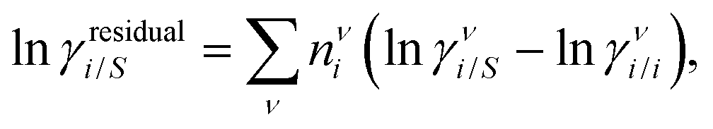
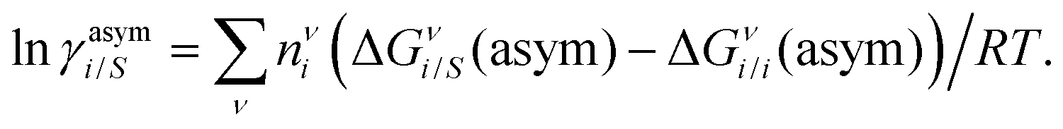
 . Since for similar types of segments the concept of asymmetric interaction between segments does not exist, so ln
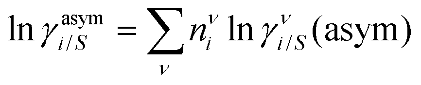 . In this model, we used the 3-suffix Margules function to capture the asymmetric interaction in terms of Margules parameters. Therefore, the expression of the excess Gibbs energy due to the asymmetric interaction can be written as
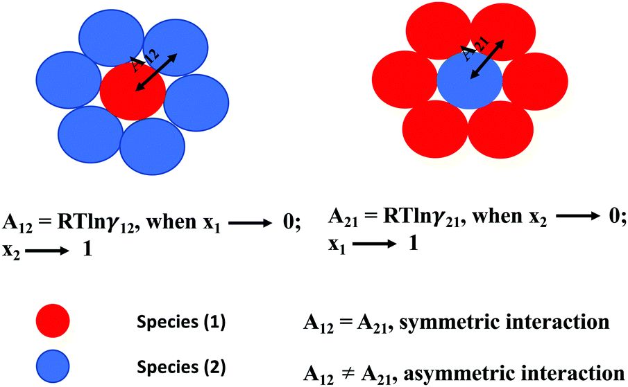
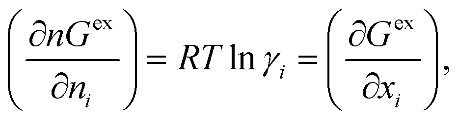
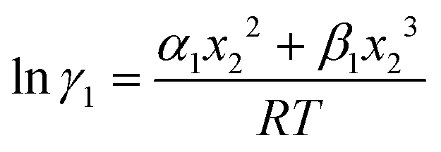
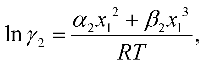
 . Hence, one can implicitly express the residual interaction within the asymmetric 3-suffix Margules function for a binary mixture. We use the activity coefficient at infinite dilution (γ∞) calculated using the COSMOSAC-201324,29 model for all binary mixture solutions used in this work. The reasons for using the COSMOSAC-2013 model are as follows (i) this is the only COSMOSAC model whose parameters are optimized over a large data set for ADF calculation,24 (ii) this is the only COSMOSAC model which includes a sophisticated dispersion interaction along with a modified residual and combinatorial term and also, (iii) this model holds an exact expression for the segment chemical potential that satisfies over all boundary conditions, and the resulting equation for the activity coefficient obeys the Gibbs–Duhem relationship to maintain thermodynamic consistency. Therefore, the basic background of the proposed model is based on the COSMOSAC-2013 model in this study. The concept of the COSMOSPACE has been used to explain the implicit definition of the residual interaction within the asymmetric term present in the “LANL” activity coefficient model within the COSMO-RS framework. The A12 and A21 cases have been shown for a spherical solute and solvent molecules in Fig. 1 which is in a hypothetical COSMOSPACE.
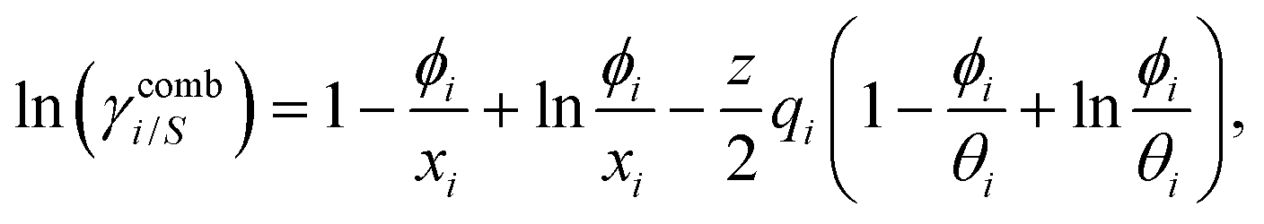
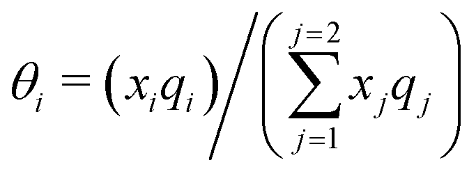 and
and 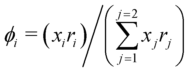 , where xi is the mole fraction of component i; ri and qi are the normalized volume and surface area parameters for species i and z is the coordination number equal to 10. zqi represents the number of nearest-neighbor sites to one of the solute and solvent molecules. In this model for the combinatorial term only the surface area qi has been normalized with q0 = 79.53. A detailed description of this SG form has been given in Section 3 in the ESI.† After adding the terms for combinatorial and asymmetric interactions described above, we obtain the expression for the activity coefficient for solute (i) and solvent (j) species in solution as:
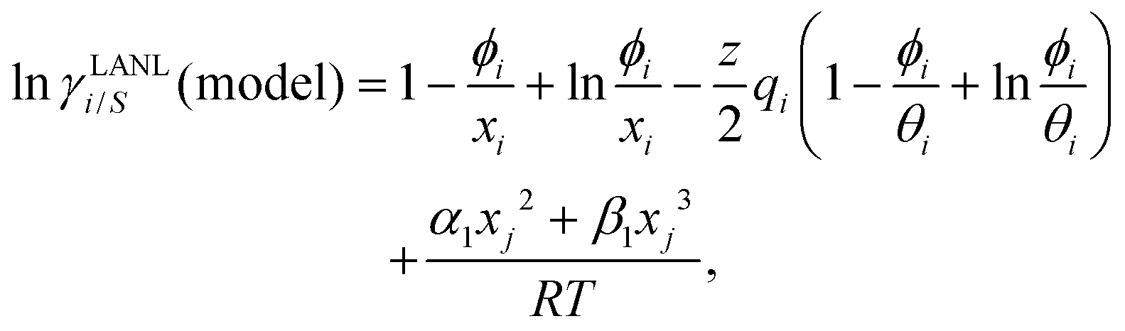
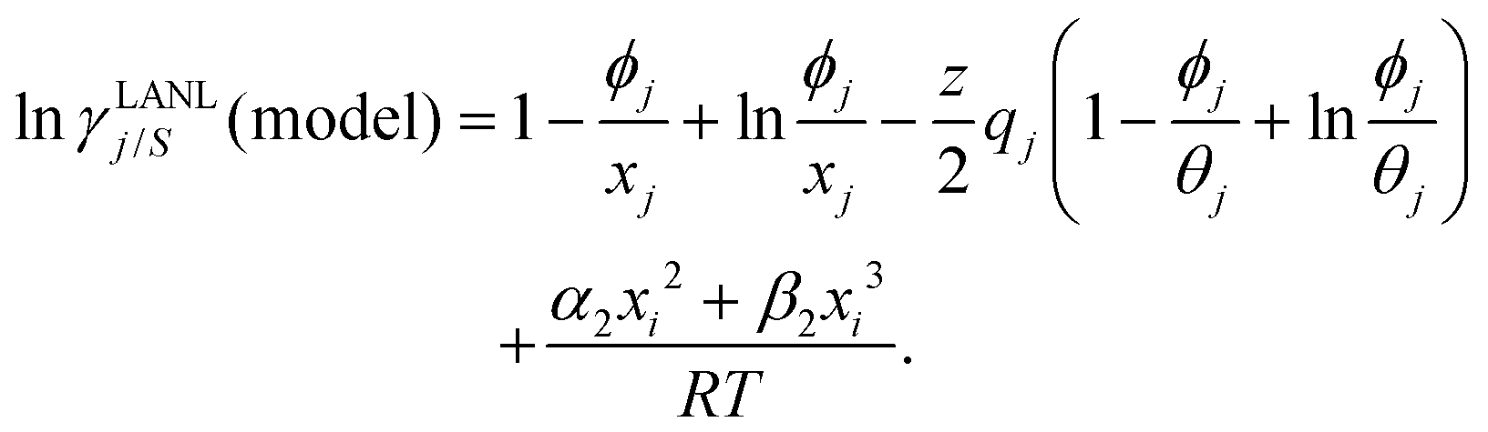
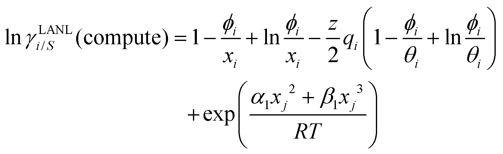

 with varying mole fractions of the solute species.1 We calculated the total excess Gibbs energy (Gex) for the binary system using the equation
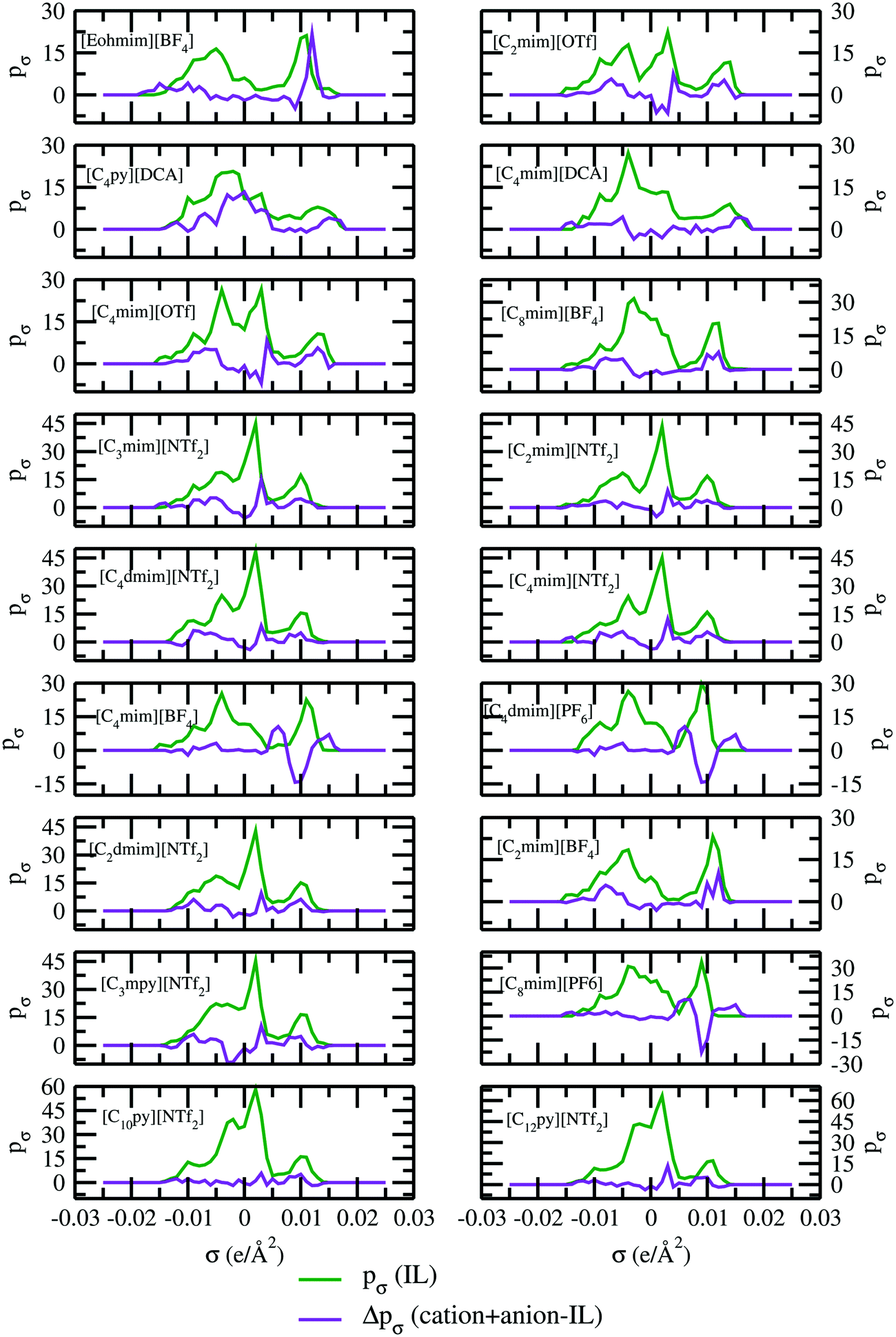
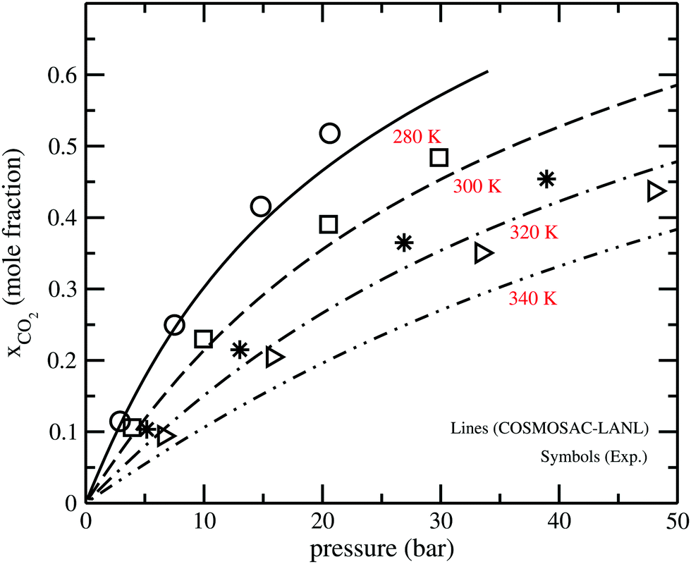
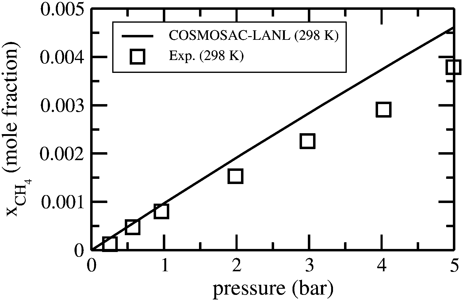
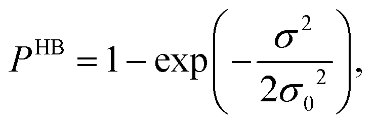
 and
and  , where Ai is the COSMO surface. The details are given in the work of Xiong et al.24 The molecules having the ability to form intermolecular hydrogen bonds between the hydroxyl (OH) group of the cation and the FB group of BF4− are the least CO2 absorbers because the physical absorption of CO2 molecules in those ionic liquids will cost high Gibbs free energy of cavity formation at the expense of breaking of intermolecular (H⋯F) hydrogen bonds. Such kind of (OH⋯OT) bond formation has been shown in Fig. 6; plot (a) indicated by a blue line, the smaller amount of (OH⋯OH) is indicated by a green line and the total of (OH⋯OT) and (OH⋯OH) is indicated by a red line and the total σ profile ptotal(σ) is indicated by a black line. Also, it is determined from the present study that the amount of (HB–OT) bond formation gradually decreases from [Eohmim][BF4] to [P66614][eFAP] with a simultaneous increase of CO2 solubility in them. The other three ILs showing medium and maximum CO2 gas solubility have no hydroxyl groups (OH). Therefore all those hydrogen bond interactions in those ILs occur due to the other than hydroxyl group (OT) interactions that are weak and these results are already seen in their corresponding σ profiles in Fig. 6; plot (b–d). The qualitative relation between the CO2 gas solubility and the inverse of the hydrogen bond interaction in an ionic liquid is in good agreement with the other results already present in this field.39–41
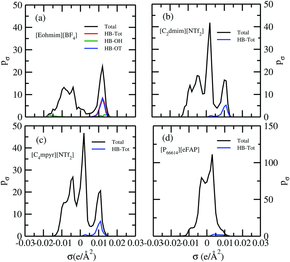
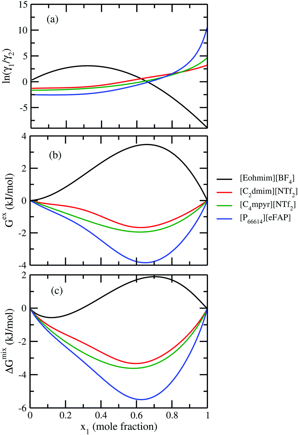
 of solute and solvent species with variation of solute mole fractions xi. The non linear curve shown in Fig. 7 arises due to the asymmetric nature of the solution, otherwise it would be a straight line.1
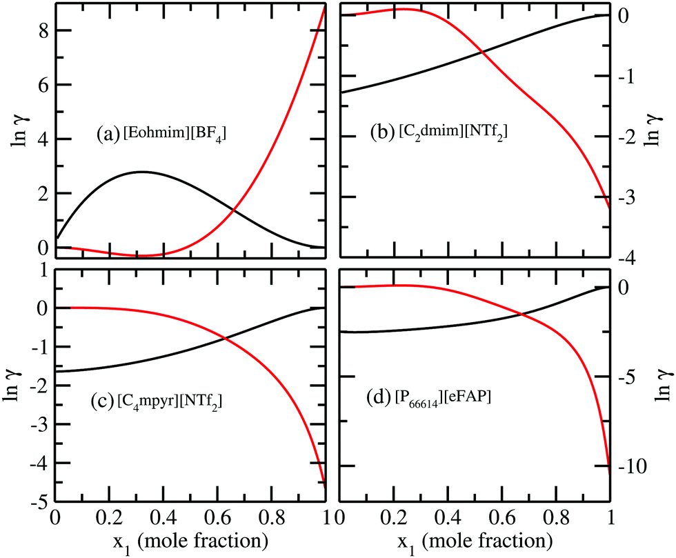
 . From Fig. 10, it is also clear that the predictive and accuracy power of the COSMOSAC-LANL model is good to produce the experimental solubility with respect to the COSMOSAC-2013 model.
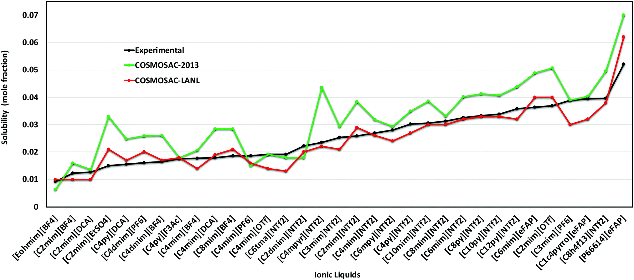
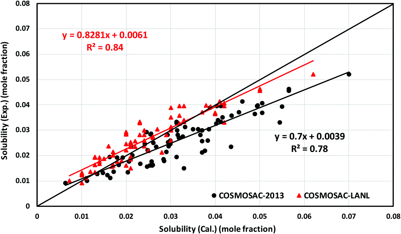

 for solubility (Henry's constant). The present model is found to improve the solubility (Henry's constant) with a minimum percentage error of 14% (16.7%) in comparison to the COSMOSAC-2013 model over a wide range of temperatures for 33 ionic liquids (over 79 data points) at 1 bar partial pressure. At room temperature, the percentage of error calculated for solubility (Henry constant) is 13% (14%). The solubility results at room temperature and for a wide range of temperatures have been given in Tables 7 and 8, respectively. From eqn (17), we know that xi = 1/Hi/S(T,P) = 1/(γ∞i/Sfi(T,P)). Therefore, Henry's constant is directly related to the activity coefficient at infinite dilution at a particular temperature. Fig. 11 shows the direct correlation between experimental solubilities and 1/γ∞i/S for both COSMOSAC-LANL and COSMOSAC-2013 models at a particular temperature and at 1 bar partial pressure. A good correlation has been observed using the new COSMOSAC-LANL model (R2 = 0.88). We also calculate the % error in the linear regression for the ideal solvation case when γCO2 = 1 for the two models at an average temperature of 298.15 K and average fugacity of 64.30 bar. The results for COSMOSAC-2013 and COSMOSAC-LANL model are 30% and 10%, respectively. The calculated percentage error in the fugacity is
  at 298.15 K. The fexpi has been calculated using the relation stated in eqn (19) at a particular temperature. The calculated average absolute relative deviations in the calculated solubilities (Henry's constant) are 12% (13%) for COSMOSAC-LANL and 27% (20%) for the COSMOSAC-2013 model, respectively, at the average room temperature (298.15 K) and at 1 bar partial pressure. The results in the form of the Henry constant have not been shown here, however the results can be obtained from the relation between the solubility and Henry's constant i.e.; xi = 1/Hi at 1 bar partial pressure in the low solubility region used in this study. The result is shown in Table S2 in the ESI.†
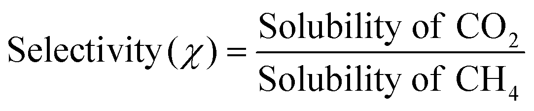 . The experimental and calculated results are given in Table 9. All the experimental results on selectivity have been taken from the references stated in the work of Lin et al.31 The present method is found to predict the selectivity between CO2 and CH4 within 12% error at a low partial pressure of 1 bar and in the low solubility region.
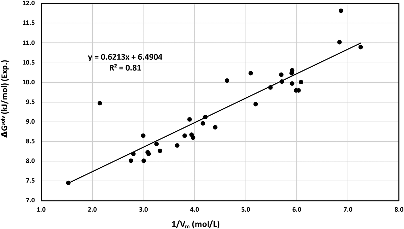
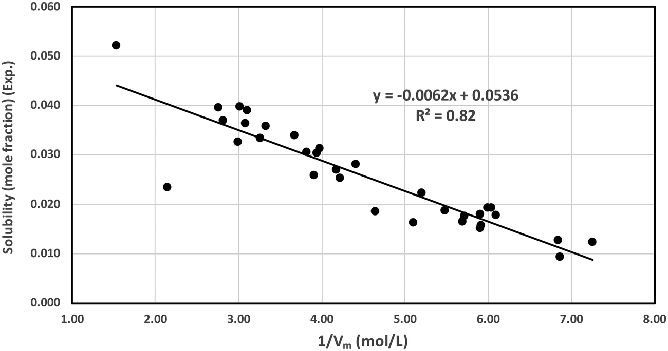
 for solute species (1). Now after adding and substituting the value of (α1 + β1) in the expression of ln
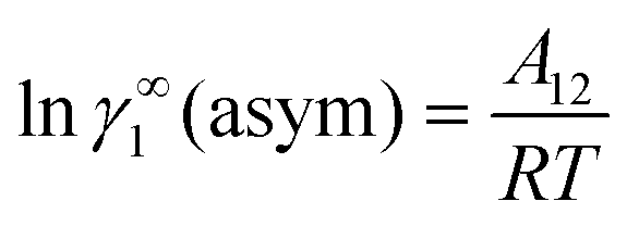 and hence,
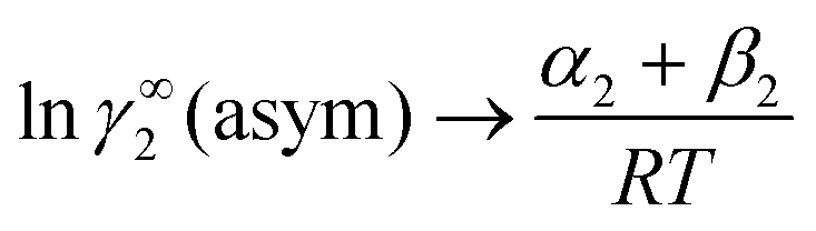 for solvent species (2). Now after adding and substituting the value of (α2 + β2) in the expression of ln
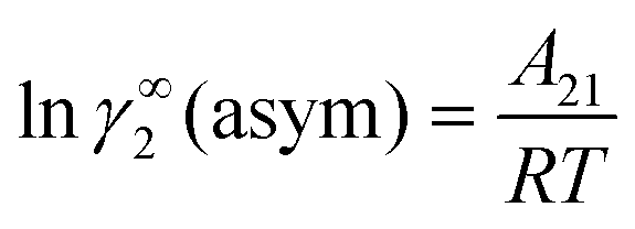 for the solvent species (2) and therefore,