
 Open Access Article
 This Open Access Article is licensed under a
 Creative Commons Attribution 3.0 Unported Licence
Spatial localization in nuclear spin-induced circular dichroism – a quadratic response function analysis†
Petr
Štěpánek
 *a and
Sonia
Coriani
b
*a and
Sonia
Coriani
b
aNMR Research Unit, Faculty of Science, University of Oulu, PO Box 3000, FI-90014 Oulu, Finland. E-mail: petr.stepanek@oulu.fi
bDTU Chemistry – Department of Chemistry, Technical University of Denmark, 2800 Kgs. Lyngby, Denmark. E-mail: soco@kemi.dtu.dk
First published on 20th May 2019
Abstract
Nuclear magneto-optic (NMO) effects are recently described phenomena originating from the interaction of light with local magnetic fields produced by nuclear spins. The phenomena border nuclear magnetic resonance and optical spectroscopy and are expected to provide rather unique spectroscopic features, borrowing from both localized response of the atomic nuclei as well as more global excitation properties of the whole molecule or its chromophore moieties. A number of quantum-chemical computational studies have been carried out, offering a reasonable agreement with nuclear magneto-optics experiments performed so far. However, the detailed structure-spectra relation is still poorly understood. In this report we address the question of locality of one of the NMO effects, namely nuclear spin-induced circular dichroism (NSCD). We implement an alternative computational approach for calculation of the NSCD intensities, based on residues of quadratic response functions, and use it to investigate the NSCD response of different nuclei in a model molecular system with well-defined separate chromophores. The results show that significant NSCD at a given energy only occurs at the nuclei which are located in the chromophore that is excited. We rationalize these findings using analysis via difference densities, and approximate sum-over-states calculations. This behaviour of NSCD opens a way to experimental studies of localization of excited states in molecules, potentially with resolution down to the order of bond-length.
1 Introduction
Nuclear magneto-optic spectroscopy (NMOS) is an umbrella term for a group of spectroscopic effects that have been experimentally and theoretically investigated in recent years. In general, NMOS effects manifest themselves as changes in polarization state of the light upon interaction with a sample possessing a macroscopic nuclear magnetization. The induced optical effect depends on the mutual orientation of the light beam and sample magnetization vector and whether the molecule is in resonance with the light beam or the effect takes place in the dispersive energy region.The first described, and so far the only experimentally observed, NMOS effect is nuclear spin-induced optical rotation (NSOR).1–5 NSOR is the rotation of the plane of polarization of linearly polarized light induced by the nuclear spin magnetization oriented along the light beam. It can be thought of as a nuclear magneto-optic analogue to Faraday rotation, a classical magneto-optic effect caused by the external magnetic field parallel with the direction of the light beam. Following the experimental observation, a number of studies on the topic of NSOR have been published,3,6–10 successfully rationalizing the measured NSOR values.
In addition to NSOR, several other NMOS effects have been theoretically predicted. These include three Cotton–Mouton-like effects: nuclear spin-induced Cotton–Mouton effect (NSCM),11,12 nuclear spin-induced Cotton–Mouton effect in external magnetic field (NSCM-B),13,14 and nuclear quadrupole-induced Cotton–Mouton effect (NQCM).15,16 Most recently, nuclear spin-induced circular dichroism (NSCD) has been theoretically investigated.17–20
NSCD is intimately connected to NSOR, stemming from the same physical origins. However, in contrast to NSOR, which is a dispersive effect, NSCD occurs at energies of electronic excitations, i.e., where the molecule has optical absorption bands. The relation between NSOR and NSCD can thus be compared to, e.g., that of optical rotation dispersion and circular dichroism in chiral compounds. Similarly, much like NSOR can be viewed as a nuclear magneto-optic analogue of Faraday rotation, NSCD can be seen as an NMO variation of magnetic circular dichroism.
It can be reasonably expected that NMOS in general should exhibit nucleus-specific features, owing to the presence of local interactions, such as the paramagnetic spin–orbit operator ĥPSO, which appears in the non-relativistic description of NSOR and NSCD.17 Such local properties have been briefly discussed before in the case of NSOR, which has been shown to provide a strong enhancement of signal near optical resonances, in a nucleus-specific manner.9 However, available theoretical analyses have dealt with this topic only in a passing manner and the experimental measurements so far have not been performed near electronic resonances in order to confirm this prediction. Moreover, it has also been shown that the overall shape of the electron density and NSCD spectra seem to qualitatively correlate,20 leading to the hypothesis that the analysis of the excited state densities may hold a key to new, nucleus-specific information hidden in NSCD.
To date, NSCD spectra have been obtained via the complex polarization propagator (CPP) approach17,18,20 also known as damped response theory.21–23 The CPP method has the advantage of taking into account contributions from all excited states at any calculated energy point, but it comes with the requirement of selecting beforehand a peak broadening parameter γ, and the need to calculate many discrete points on a frequency grid to obtain a sufficiently smooth spectral curve. Moreover, in order to extract the NSCD contribution from a particular excited state, one needs to resort to numerical fitting of the CPP curve.20 The results of such fitting are prone to errors due to the fact that even low energy regions of the CPP curve contain contributions from “tailing” peaks of excited states lying at higher energies.
The purpose of this study is twofold:
First, we present an alternative method to CPP for calculating NSCD, based on residues of quadratic response functions,24–26 to tackle the issue of obtaining analytical NSCD intensities for individual excited states. This approach allows us to calculate the NSCD intensity in a manner similar to calculations of the B term of magnetic circular dichroism.25–27
Second, we use this alternative response function formalism as well as a sum-over-states approach, to investigate the NSCD response with respect to the location of the nuclei within the excited chromophore. We note in passing that even if both approaches to large extent build upon existing response function residue computational machinery, the specific formulas for NSCD were derived and coded for the first time for this work. The results show that the strongest NSCD signals come from nuclei in the regions of significant electron density changes during excitation. The NSCD can thus in practice offer an experimental tool to probe, nucleus by nucleus, the spatial extent of electronic excitations.
2 Methods
2.1 NSCD intensities from residues of quadratic response functions
The NSCD ellipticity (per unit sample length, spin polarization, and nuclear concentration) has earlier been shown17 to be given by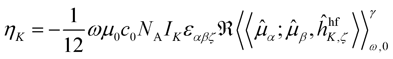 | (1) |
![[small mu, Greek, circumflex]](https://www.rsc.org/images/entities/i_char_e0b3.gif) α;β,ĥhfK,ζ〉〉γω,0 indicates the damped complex quadratic response function of the (Cartesian components α, β and ζ of) electric dipole
α;β,ĥhfK,ζ〉〉γω,0 indicates the damped complex quadratic response function of the (Cartesian components α, β and ζ of) electric dipole 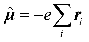 and hyperfine interaction ĥhfK operators. The latter corresponds, in non-relativistic theory and for a closed shell system, to the paramagnetic spin–orbit operator
 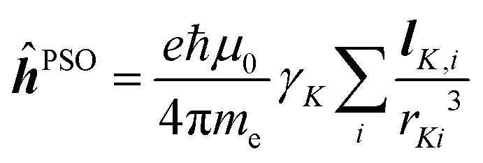 , with lK,i as the angular momentum of electron i about the position RK of nucleus K.
The expression in eqn (1) was derived by analogy with the one for the Magnetic Circular Dichroism (MCD) ellipticity (per unit sample length, concentration and magnetic field strength)26,28
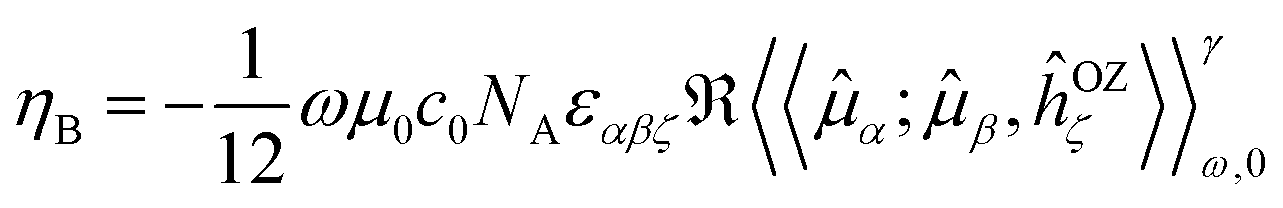 | (2) |
εαβζℜ〈〈α;β,ĥOZζ〉〉γω,0 = 2![[scr B, script letter B]](https://www.rsc.org/images/entities/char_e13f.gif) (0 → f)af(ω,ωf) (0 → f)af(ω,ωf) | (3) |
(0 → f) is known as “the B term of MCD”,27,30,31 for a transition from (ground) state 0 to excited state f, and af(ω,ωf) is a (Lorentzian) line-shape function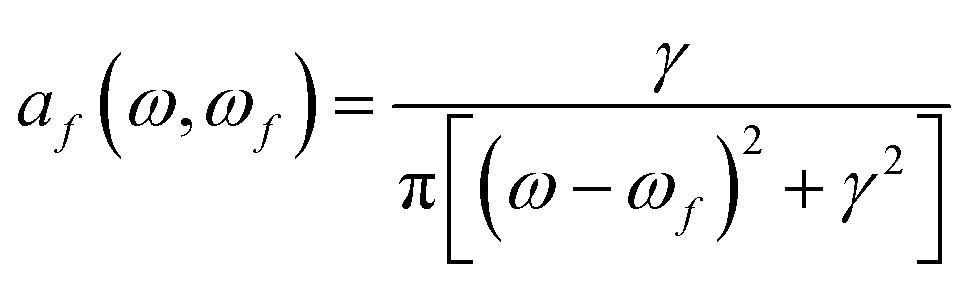 | (4) |
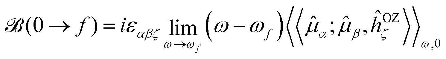
A sum-over-state expression for (0 → f) was derived long ago by Stephens and Buckingham,30–32 and it has previously been shown to be attainable from the single residues of (standard) quadratic response functions24–26,29
 | (5) |
α|f〉〈f|β|0〉,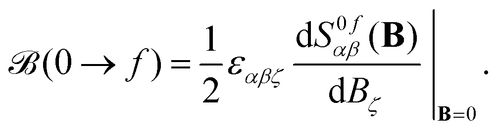 | (6) |
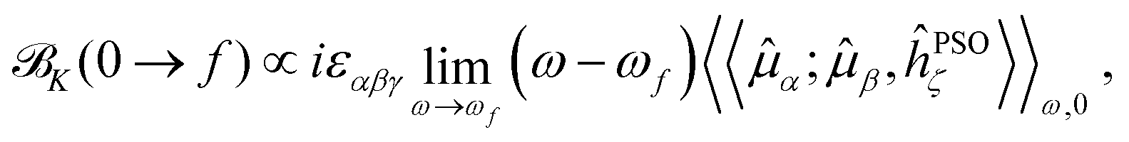
The expression in eqn (5) allows one to straightforwardly decompose and rationalize the MCD spectral bands in terms of (signed) intensity sticks associated with specific electronic transitions 0 → f. To take advantage of a similar possibility for the NSCD signals, we introduce here the NSCD B term, K(0 → f), and compute it via residues of the regular quadratic response functions 〈〈![[small mu, Greek, circumflex]](https://www.rsc.org/images/entities/b_i_char_e0b3.gif) ;,ĥPSOK〉〉ω,0
;,ĥPSOK〉〉ω,0
 | (7) |
The results were checked for consistency by comparing the computed (total) ellipticity spectrum of (active) nucleus K (per unit path length and unit of spin polarization) obtained as
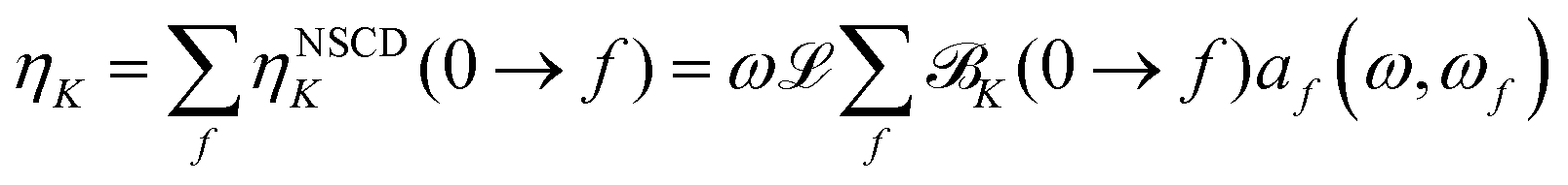 | (8) |
K(0 → f)} using the same value of the (inverse) life-time parameter γ used in the CPP calculations. The prefactor ![[script L]](https://www.rsc.org/images/entities/char_e144.gif) in eqn (8) is a product of physical constants, see ESI.†
in eqn (8) is a product of physical constants, see ESI.†
2.2 Computational details
All molecular structures were optimized using Turbomole 7.0.2 at B3LYP/def-TZVP/vacuum level with m5 grid37,38 using available symmetry point groups (D2h for ethene, C2v for water and pyridine, D6h and benzene, Cs for the model system described below). The local minimum geometry was confirmed by calculations of the harmonic vibrational frequencies. The choice of method for calculation of excitation properties and NSCD depended on the purpose of the calculation, differing between benchmark tests and production calculations for investigations of the NSCD localization.2.3 Theoretical models
| Molecule | Method | Basis set |
|---|---|---|
| Ethene | HF | 6-31G |
| Ethene | DFT/BHandHLYP | 6-31G |
| Ethene | DFT/BHandHLYP | def-SVPDD-0 |
| Water | DFT/B3LYP | aug-cc-pVTZ |
| Pyridine | HF | 6-31G |
| Benzene | HF | 6-31G |
The excitation energies and NSCD intensities for investigations of localization of the NSCD response in our model molecule (vide infra) were calculated using the BHandHLYP functional with the def2-SVPDD-0 basis set,20 with a development version of DALTON.34,35
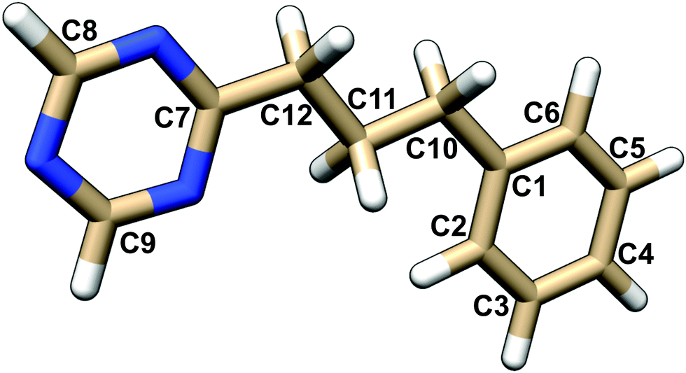 | ||
| Fig. 1 Atom numbering of the PPT molecule. | ||
The strength of the calculated NSCD signal of the individual nuclei has been assessed with respect to the local electronic density changes ρdiff,f upon excitation, defined as
| ρdiff,f = ρf − ρ0 | (9) |
Molecular visualizations were prepared using the UCSF Chimera package.42
3 Results
3.1 Benchmarking the B-term formalism
As anticipated in the Methods section, the new implementation was tested for consistency via comparison of NSCD computed viaeqn (7) and (8) with that obtained using the CPP protocol. The NSCD termsK(0 → f) for excited states f calculated via the B-term-like formalism have been broadened by the Lorentzian band of the same half-width γ = 0.00456EH = 1000 cm−1 as used in the CPP calculations, according to eqn (8).
The results for ethene and pyridine at the HF/6-31G level are shown in Fig. 2. Clearly, the new B-term formalism allows to faithfully reproduce the CPP curve. Moreover, in this case of rather well separated excited states, the calculation is much more efficient than with CPP, resulting in significant reduction of computational time. It should be noted, however, that this advantage may not hold for systems with many closely spaced excited states or when a high-energy region of the spectrum is desired, since in that case many lower lying excited states would need to be evaluated, potentially making the B-term calculation too demanding. Moreover, the CPP approach is robust even in cases of degenerate states, where the residue approach may become numerically unstable. This is for instance the case for benzene in a fully symmetric D6h geometry. For molecules belonging to the D6h point group, degenerate electronic excited states occur, leading to divergent NSCD B-term values, on account of a vanishing energy difference in the denominator (see eqn (11) below). At the same time, degenerate excited states give rise to A-term type of signals, which can indeed be regarded as special occurrences of the B terms, stemming from the excitation to a degenerate excited state.29 The signals due to the A terms can be pragmatically obtained as pseudo-A terms by computing the B-term contributions at a slightly distorted geometry,43 see ESI.† Additional benchmark tests with similar level of agreement are shown in ESI.†
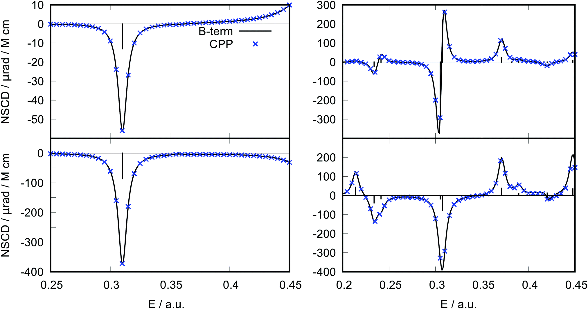 | ||
| Fig. 2 Comparison of the NSCD signal of hydrogen (top) and carbon (bottom) atoms calculated via the CPP approach (blue crosses) with the spectrum produced via the B-term formalism (black solid line) at HF/6-31G level. The left panels show results for ethene and the right ones for atoms in ortho-position in pyridine. Fifteen states have been calculated in the B-term approach for ethene and twenty for pyridine. A Lorentzian band with the same broadening parameter as used in the CPP calculation (γ = 0.00456 a.u. = 1000 cm−1) was used to simulate the spectrum. | ||
As a second example, we have performed ad hoc comparisons of NSCD results for two carbon atoms (C1 and C7) of the PPT molecule (Fig. 3). It is apparent how inclusion of the K terms from more excited states into the spectral ellipticity curve improves the convergence of the results towards the CPP result. It can be seen in the case of C7 that even excited states 13 to 17 contribute to the spectral curve in the lower energy region, showing the effect of “tailing”.
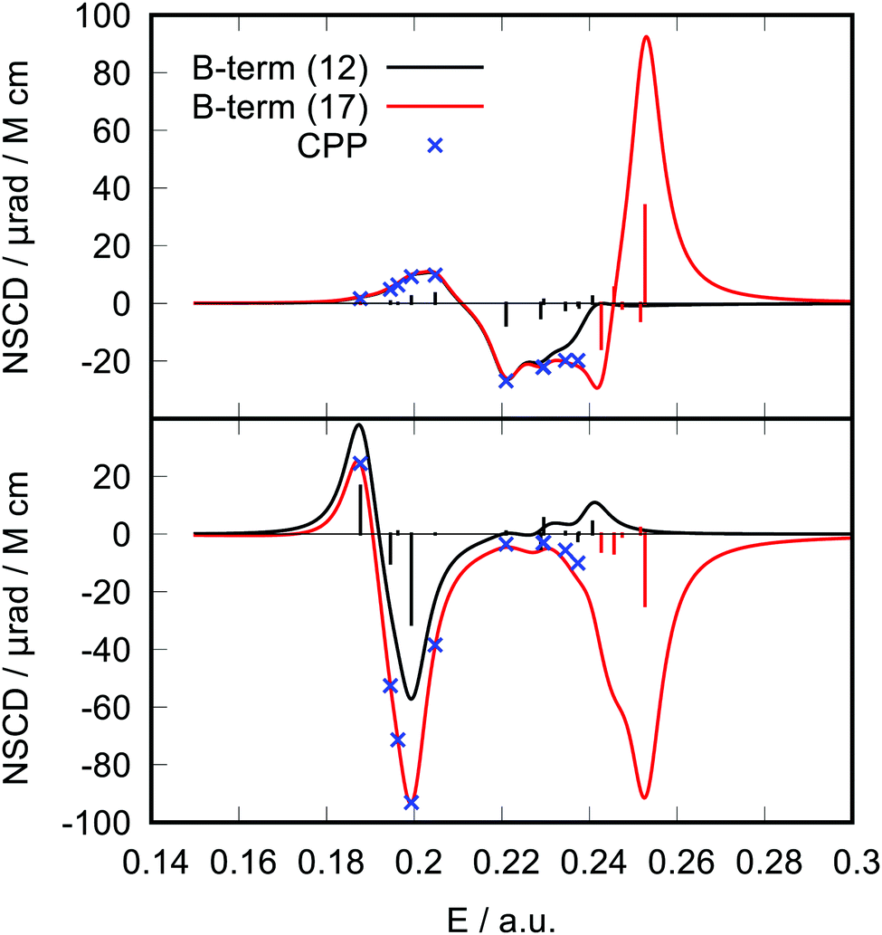 | ||
| Fig. 3 Model molecule PPT. Comparison of the NSCD signal of carbon atom C1 (top panel) and C7 (bottom panel) calculated via the CPP approach (blue crosses) with the spectrum produced via the B-term approach. Two curves represent results for 12 (black line) or 17 (red line) excited states. A Lorentzian broadening with the same broadening parameter as used in the CPP calculation (γ = 0.00456 a.u. = 1000 cm−1) was used to simulate the spectrum. | ||
Based on these results, we conclude that the B-term computational protocol provides correct NSCD intensities and signs and can be reliably used for the analysis presented in the following sections.
3.2 Localization of NSCD in molecules
The model for our investigation of locality of NSCD was the PPT molecule. The properties of its first nine excited states are summarized in Table 2 and their difference densities are shown in Fig. 4. As can be clearly seen, the first four excitations are localized in the triazine moiety, while the following three are in the phenyl ring. Higher excitations are delocalized over the whole molecule. The numbers in Fig. 4 indicate the calculated strengths of the NSCD B terms, multiplied by 1000 for convenience.| Excitation | Symmetry | Energy/eV | f × 103 | Excitation localization |
|---|---|---|---|---|
| 1 | A′′ | 5.11 | 8.39 | Triazine |
| 2 | A′′ | 5.29 | 1.43 | Triazine |
| 3 | A′′ | 5.34 | 0.21 | Triazine |
| 4 | A′′ | 5.43 | 4.77 | Triazine |
| 5 | A′ | 5.57 | 2.97 | Phenyl |
| 6 | A′ | 6.01 | 29.86 | Phenyl |
| 7 | A′′ | 6.24 | 2.20 | Phenyl |
| 8 | A′ | 6.25 | 6.11 | Delocalized |
| 9 | A′ | 6.38 | 5.14 | Delocalized |
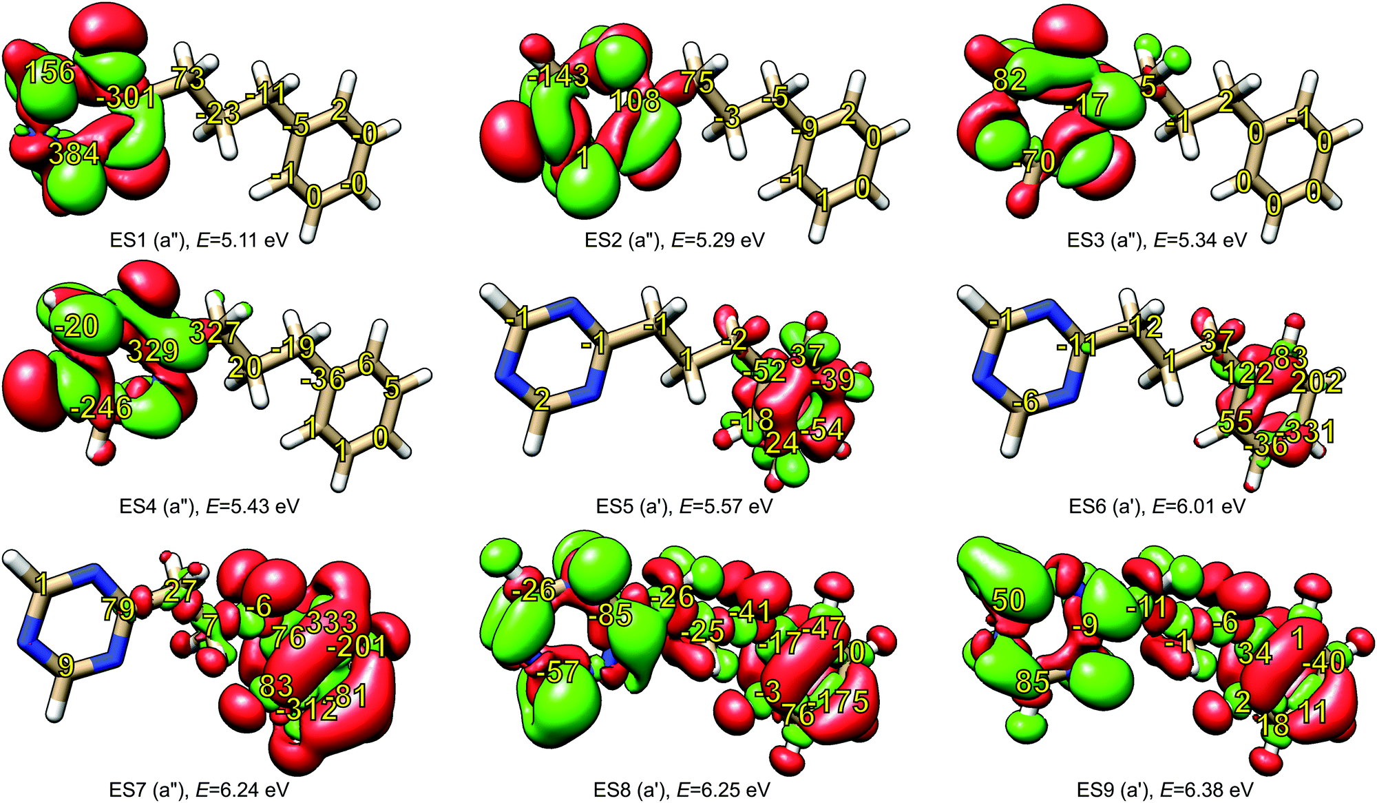 | ||
| Fig. 4 Excited state difference densities of the first nine excited states of PPT model molecule (isovalues ±0.001). The symmetry of the excited state and its excitation energy are shown for each state. Yellow numbers indicate NSCD B terms K for individual carbon atoms (multiplied by a factor of 1000 for easier readability). | ||
A trend can be observed in Fig. 4. In the case of the first excited state, the carbon atoms of triazine show two orders of magnitude larger NSCD B terms than the ones in the phenyl group. In addition, the magnitude of the NSCD for the carbon atoms forming the bridge between the two chromophores decreases going from the triazine side towards the phenyl. A somewhat similar situation is observed in the case of the second excited state, with the remarkable exception of the carbon nucleus C9 in triazine, that shows negligible NSCD. The third excited state also shows stronger signals in the excited chromophore, although the absolute numbers are smaller than in the previous cases, likely because of the small oscillator strength, which modulates the total NSCD intensity of the transition (see eqn (11) below). Likewise, the fourth state behaves in comparable manner, with the NSCD signal also significantly extending towards the adjacent bridge atom. On the other hand, excited states 5, 6 and 7, which are localized on the phenyl ring, manifest strong NSCD signals for the phenyl ring carbon nuclei and much smaller ones for the nuclei located in triazine. Excited states 8 and 9 are spread around the whole molecule and likewise is the overall NSCD intensity.
From these observations, a tentative conclusion can be made: the excited state location, determined through electron density changes, influences the magnitude of the NSCD response for the individual nuclei. In general, large NSCD signals appear in the regions of significant changes in electron density upon excitation. This behaviour is consistent with our previous observation, where atoms located outside of the chromophore showed significantly lower NSCD compared to those located within.20
It should be noted, however, that large change in the local electron density is apparently a necessary, but not sufficient, condition for large NSCD, since in some individual cases, small NSCD could be observed even in such regions.
3.3 Rationalization of the NSCD relation to the electron density
It is worth discussing the underlying origin of the correlation between the local electron density and the NSCD magnitude. The expression for the NSCD signal of a particular nucleus K and electronic transition from ground state 0 to excited state f was implicitly given in eqn (8)17,20| ηK(0 → f) = ωKK(0 → f)af(ω,ωf) | (10) |
The K(0 → f) has the SOS expression
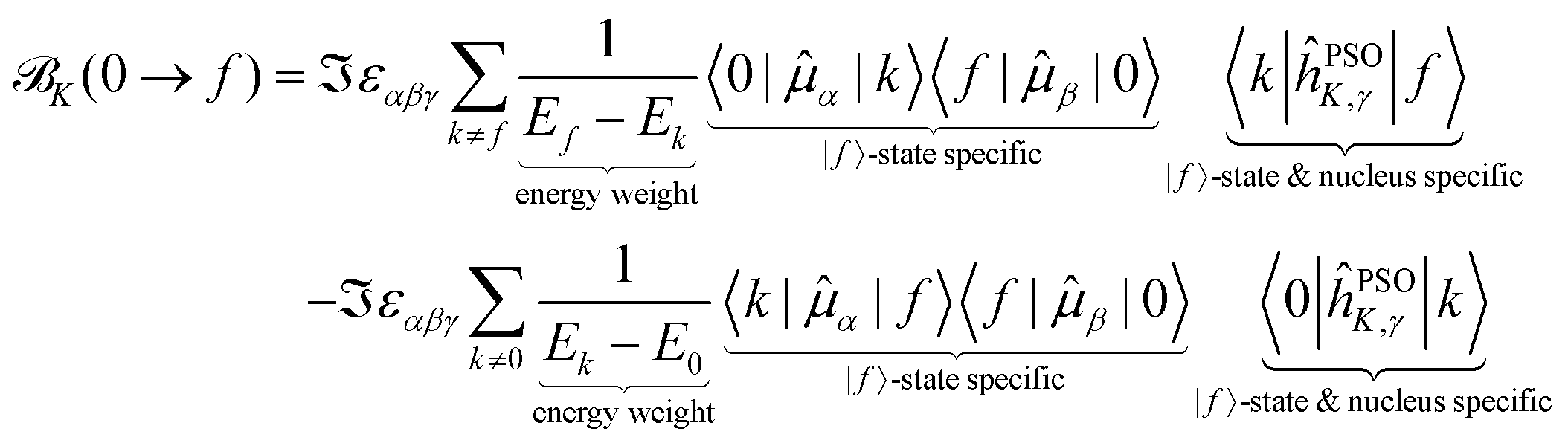
 | (11) |
Starting from eqn (11), we can isolate the term k = 0 in the first summation, and the term k = f in the second one
 | (12) |
The last term connects the NSCD intensity for the excited state f to the difference in expectation value of the electric dipole moment operator (component) between the ground state 0 and the excited state f. Each expectation value can be written as contraction of the dipole moment integrals with the one particle density matrix of the given state, whereas the electron density for each state in eqn (9) is a contraction of the density matrix of that state with two orbitals. Thus the two quantities, density differences in eqn (9) and dipole moment differences in eqn (12), are related via the density matrix differences. Values of the last term in eqn (12) for the first nine excited states and all carbon atoms of PPT are plotted in Fig. 5.
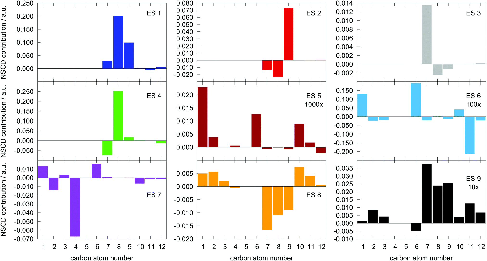 | ||
Fig. 5 Magnitude of 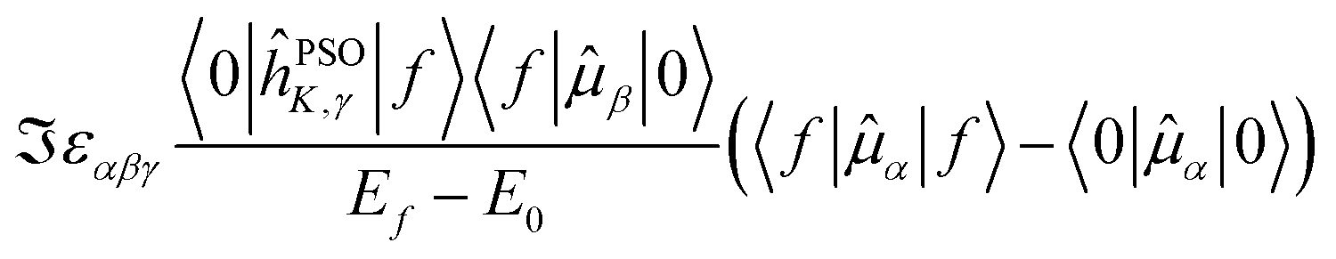 (the term on the last line of eqn (12)) for the first nine excited states for all carbon atoms of the PPT molecule. Numbers in panes of excited states 5, 6, and 9 indicate multiplication factor for those values. (the term on the last line of eqn (12)) for the first nine excited states for all carbon atoms of the PPT molecule. Numbers in panes of excited states 5, 6, and 9 indicate multiplication factor for those values. | ||
As can be seen, there is a correspondence between the appearance of appreciable NSCD signals and the size of this “density difference term”. However, it should be noted that the differences in dipole moments do not refer to any specific nucleus by themselves and thus can not be responsible for the differences between different atoms. That is modulated by the element 〈0|ĥPSOK|f〉, as we will demonstrate below.
| |f〉 = |fT,fP〉 | (13) |
Due to the local nature of the operator ĥPSOK acting on nucleus K, we can then approximate the corresponding matrix elements taking into account only the electronic state of the chromophore to which the specific nucleus belongs. Thus, for example, integral 〈0|ĥPSOC1|1〉 for nucleus C1, which is in the phenyl chromophore, reduces to
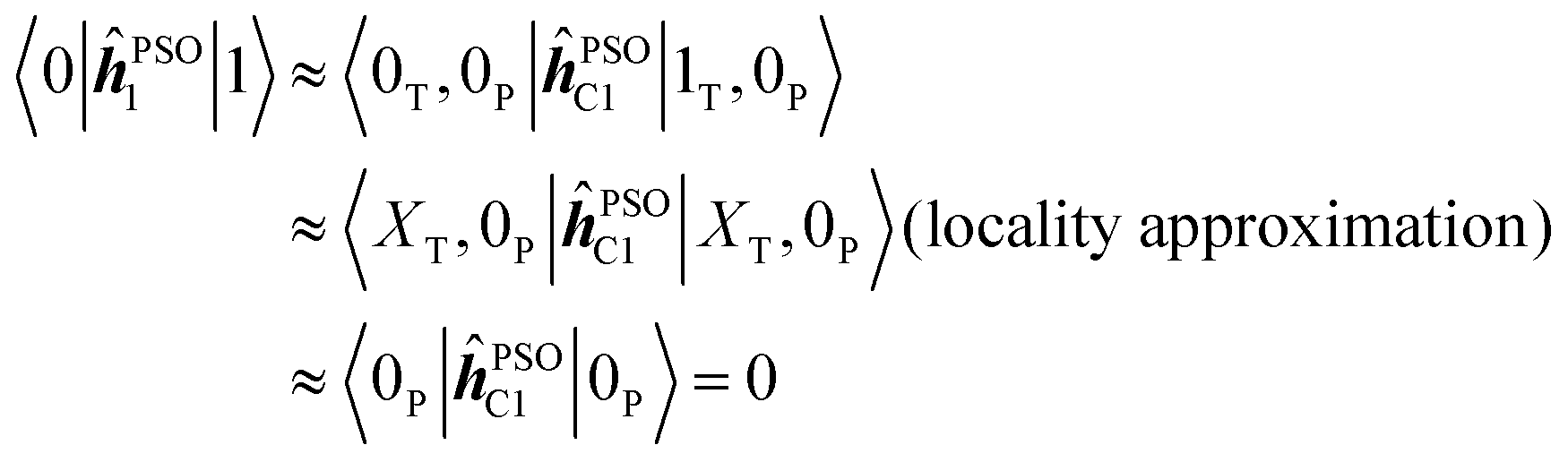
Based on this argument, integrals of the form 〈i|ĥPSOK|j〉 can only be significant if the states i and j differ locally in the vicinity of nucleus K. From Fig. 4, we can see that, for example, states 0, 1, 2, 3 and 4 can not mutually produce significant integrals for nuclei in the phenyl group since they all share locally the same ground state density. The same argument applies to states 5, 6 and 7 for the case of triazine ring.
In short, this effectively means that if the nucleus K resides on a non-excited chromophore, the element 〈0|ĥPSOK|f〉 is small and the state is “locked out” of interaction with several energetically close excited states, that all share locally unexcited ground-state wavefunction. On the other hand, the excited chromophore does not face such restrictions as excited state densities are, in general, different from both ground state, as well as from one another.
3.4 Relative significance of individual operators and their integrals
Expanding on the previous section, we can present yet another qualitative picture of the dependence of NSCD on the local properties in terms of the relative magnitudes of different molecular integrals appearing in the expression for the NSCD.For this purpose, we interpret eqn (11) in literal sum-over-states terms. First, we need to assess the level of agreement between the B-term (QR-residue) and sum-over-states calculations. Fig. 6 shows the correlation of NSCD calculated using the two approaches for the first ten excited states and all twelve carbon atoms (120 points in total, 100 excited states used in the summation). As can be seen, the results are not completely converged even for 100 states, but they are steadily improving with the number of states (see ESI†). Nevertheless, there is a significant semi-quantitative agreement justifying our following discussion.
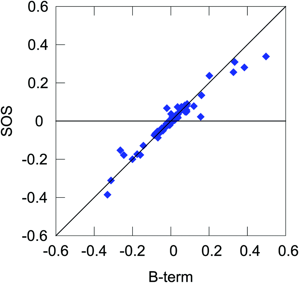 | ||
| Fig. 6 Correlation between NSCD calculated using the B-term approach and the sum-over-states expression with 100 excited states. The plot shows all NSCD values for the first ten final excited states for all twelve carbon atoms. | ||
We can expand and partition the NSCD expression in eqn (11) in the following way
 | (15) |
The first point to note is that the reciprocal energy prefactor on each line governs the overall weight of the individual contribution to NSCD. The energy differences between two excited states appearing on the first line can be arbitrarily small, and closely spaced excited states will thus in general contribute more than ones lying farther apart. On the other hand, the expression on the second line is weighted by the reciprocal value of the excited states energies. The latter are commonly sizable values, and their reciprocal value will then be (relatively) small. For example, in the current case of PPT, the lowest excitation energy is 5.11 eV, while the energy separation of the individual excited states is on the order of 0.1 eV. Thus, the terms on the first line have much larger overall weight.
Since a detailed analysis of the interplay of the molecular integrals based on full expansion of such expression becomes quickly rather cumbersome for more than a few states, it might be prudent to construct some auxiliary measure that would capture qualitative differences of various contributions. For this purpose, sums of magnitudes of four matrix elements appearing in eqn (12), i.e. linear and quadratic response function residues for both operators, have been calculated. The sums are summarized in Table 3 along with some of their basic properties that will be discussed. The table indicates the spatial nature of the matrix element, where elements with the ĥPSOK operator are deemed “local” due to their r−3 dependence on the distance from their respective nuclei, and elements with electric dipole moment operator are described as “global” to reflect their independence on the specific nucleus.
| Sum of matrix elements | Spatial extent | # of identical elements when f → g |
|---|---|---|
|
Global | n − 2 |
|
Global | 1 |

|
Local | n − 2 |
|
Local | 0 |
The choice of the sums being composed of these four types of molecular integrals is motivated by the following: (a) they are four naturally occurring components in the expression for NSCD (eqn (11)); (b) they have different spatial extent (“local” vs. “global”); (c) they differ in the extend to which their values change when the final excited state f changes f → g, since they stem from either linear or quadratic response functions. Summing together their absolute magnitudes thus gives some qualitative insight into the relative significance of that particular type of integral in determining of the NSCD values for different excited states and nuclei.
We stress again that these sums are only a qualitative tool that does not correlate directly with the NSCD intensity, as the latter contains the mixed products of such matrix elements. Nevertheless, the sums can be used as auxiliary measures of the variability of the average total magnitude of individual elements appearing in the expression for NSCD intensity, with respect to different excited states f and nuclei K. The properties of some of these sums can be inferred at a glance, whereas for others they are more involved and we thus present them graphically in Fig. 7. Let us inspect them.
 | ||
Fig. 7 Averages of absolute values of different integrals for k ∈ {first 100 excited states}: (a)  (top, left); (b) (top, left); (b) 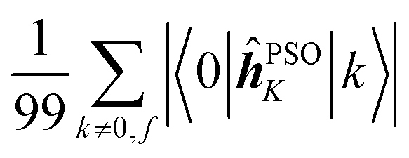 (top, right); (c) (top, right); (c) 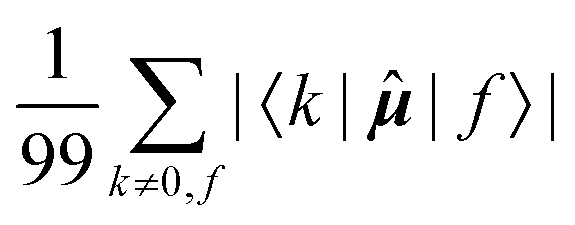 (bottom, left); (d) (bottom, left); (d) 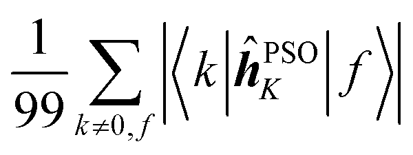 (bottom, right). Each vertical line for a specific carbon nucleus (as indicated by the number in abscissa) corresponds to one of the first nine excited states f. (bottom, right). Each vertical line for a specific carbon nucleus (as indicated by the number in abscissa) corresponds to one of the first nine excited states f. | ||
The elements 〈0||k〉 form a sum that is obviously independent of the nucleus and is only slightly dependent on the final excited state f. The dependence arises because sums are composed of (n − 1) identical terms, except for a single element 〈0||f〉, which is excluded in each case. In comparison, elements of the form 〈k||f〉 sum to a quantity that is, predictably, also nucleus-independent, but depends strongly on the final state f. This is due to the fact that all (n − 1) elements 〈k||f〉 in the summation are different for different states f, with the exception of the pair 〈k||f〉 = 〈f||k〉 which naturally appears also when roles of states k and f in the summation are exchanged.
Concerning the ĥPSOK operator, it can be seen that the quantity  is dependent on the final excited state f only through a single element (as discussed above for the dipole moment operator), but predictably depends considerably on the nucleus. This is expected as the operator is nucleus-specific. Finally, the sums of elements of the form 〈k|ĥPSOK|f〉 exhibit the largest variation in magnitude both between excited states as well as between individual nuclei. This is a consequence of ĥPSOK being a nucleus-specific operator and every single element in the sum changing for different final state f.
Remarkably, it can also be seen that the variation in intensity of this sum somewhat correlates with the intensity of NSCD for a particular combination of nucleus and excited state. It should be pointed out again, that since the elements 〈k|ĥPSOK|f〉 are combined with other contributions, the sum does not correlate with the actual NSCD intensity, but merely gives the qualitative information about the relative importance of the excited states at the site of the probed nucleus. Of particular interest here is excited state number 2 for nucleus C9. As it was pointed out in the discussion of Fig. 4, this nucleus resides inside the volume of large density change, but it exhibits very weak NSCD. As it can be seen here, the magnitudes of the 〈2|ĥPSOC2|k〉 elements are significant. However, due to their combination with other smaller integrals in the sum and variation in signs, the net result is accidentally almost vanishing in this particular case.
The results suggest that the integrals 〈k|ĥPSOK|f〉 play a significant role in determining the total NSCD intensity due to their sensitivity to both to excited states as well as different nuclei. This effect appears to be a necessary, if not sufficient, condition for appreciable NSCD and its impact is potentially further enhanced by the large reciprocal energy weighting prefactor.
4 Conclusions
We have presented a new computational protocol for calculating excited-state specific, B-term-like, contributions to the NSCD ellipticity. The approach is based on single residues of quadratic response functions involving two electric dipole and one PSO operators and it allows to analytically evaluate the NSCD for a given electronic transition. Benchmark tests have shown that the values thus obtained yield NSCD spectra identical to the ones calculated via a previously established complex polarization propagator approach.Using the new method, we have investigated the question of local nature of the excitation in NSCD and its relation to the signal from the nuclei residing in the chromophore being excited. The results show that the strong NSCD signals form only for nuclei residing in the excited chromophores, defined as a place of significant change in electronic density. The findings were rationalized based on an analysis of the individual terms contributing to the NSCD intensities, and found to originate from the ĥPSOK operator due to its localized nature. In particular, second order perturbations involving two excited states appear to be important for correct description of this phenomenon.
The presented results show that NSCD has the ability to distinguish between nuclei based on their location in different chromophores. This opens up interesting possibilities for a two-dimensional nuclear-resonance/optical-resonance spectroscopy for probing localization of excitation states in molecules. The results also establish a basis for a rational search for suitable molecular systems to target in first observations of this exciting phenomenon.
Conflicts of interest
There are no conflicts to declare.Acknowledgements
This project has received funding from the European Union's Horizon 2020 research and innovation programme under the Marie Skłodowska-Curie grant agreement NMOSPEC, No. 654967 (P. Š.) and ETN COSINE, No. 765739 (S. C.). We also thank the Magnus Ehrnrooth Foundation for financial support (P. Š.). The authors acknowledge financial support from the Kvantum institute (University of Oulu) and from Academy of Finland (Grant 316180) (P. Š.). We acknowledge grants of computer capacity from the Finnish Grid and Cloud Infrastructure (persistent identifier urn:nbn:fi:research-infras-2016072533). S. C. acknowledges support from DTU Chemistry and from the Independent Research Fund Denmark – DFF-Forskningsprojekt2 grant no. 7014-00258B.References
- I. M. Savukov, S. Lee and M. V. Romalis, Nature, 2006, 442, 1021–1024 CrossRef CAS PubMed.
- I. M. Savukov, H. Chen, T. Karaulanov and C. Hilty, J. Magn. Reson., 2013, 232, 31–38 CrossRef CAS PubMed.
- J. Shi, S. Ikäläinen, J. Vaara and M. V. Romalis, J. Phys. Chem. Lett., 2013, 4, 437–441 CrossRef CAS PubMed.
- D. Pagliero and C. A. Meriles, Proc. Natl. Acad. Sci. U. S. A., 2011, 108, 19510–19515 CrossRef CAS PubMed.
- D. Pagliero, W. Dong, D. Sakellariou and C. A. Meriles, J. Chem. Phys., 2010, 133, 154505 CrossRef PubMed.
- S. Ikäläinen, M. V. Romalis, P. Lantto and J. Vaara, Phys. Rev. Lett., 2010, 105, 153001 CrossRef PubMed.
- G. Yao, M. He, D. Chen, T. He and F. Liu, Chem. Phys., 2011, 387, 39–47 CrossRef CAS.
- T. S. Pennanen, S. Ikäläinen, P. Lantto and J. Vaara, J. Chem. Phys., 2012, 136, 184502 CrossRef PubMed.
- S. Ikäläinen, P. Lantto and J. Vaara, J. Chem. Theory Comput., 2012, 8, 91–98 CrossRef PubMed.
- J. Vähäkangas, P. Lantto and J. Vaara, J. Phys. Chem. C, 2014, 118, 23996–24005 CrossRef.
- T. Lu, M. He, D. Chen, T. He and F. Liu, Chem. Phys. Lett., 2009, 479, 14–19 CrossRef CAS.
- L. Fu and J. Vaara, J. Chem. Phys., 2013, 138, 204110 CrossRef PubMed.
- G. Yao, M. He, D. Chen, T. He and F. Liu, ChemPhysChem, 2012, 13, 1325–1331 CrossRef CAS PubMed.
- L. Fu and J. Vaara, ChemPhysChem, 2014, 15, 2337–2350 CrossRef CAS PubMed.
- L. Fu, A. Rizzo and J. Vaara, J. Chem. Phys., 2013, 139, 181102 CrossRef PubMed.
- L. Fu and J. Vaara, J. Chem. Phys., 2014, 140, 024103 CrossRef PubMed.
- J. Vaara, A. Rizzo, J. Kauczor, P. Norman and S. Coriani, J. Chem. Phys., 2014, 140, 134103 CrossRef PubMed.
- M. Straka, P. Štěpánek, S. Coriani and J. Vaara, Chem. Commun., 2014, 50, 15228–15231 RSC.
- F. Chen, G. H. Yao, Z. L. Zhang, F. C. Liu and D. M. Chen, ChemPhysChem, 2015, 16, 1954–1959 CrossRef CAS PubMed.
- P. Štěpánek, S. Coriani, D. Sundholm, V. A. Ovchinnikov and J. Vaara, Sci. Rep., 2017, 7, 46617 CrossRef PubMed.
- P. Norman, D. M. Bishop, H. J. A. Jensen and J. Oddershede, J. Chem. Phys., 2001, 115, 10323–10334 CrossRef CAS.
- P. Norman, D. M. Bishop, H. J. A. Jensen and J. Oddershede, J. Chem. Phys., 2005, 123, 194103 CrossRef PubMed.
- J. Kauczor and P. Norman, J. Chem. Theory Comput., 2014, 10, 2449–2455 CrossRef CAS PubMed.
- J. Olsen and P. Jørgensen, J. Chem. Phys., 1985, 82, 3235–3264 CrossRef CAS.
- S. Coriani, P. Jørgensen, A. Rizzo, K. Ruud and J. Olsen, Chem. Phys. Lett., 1999, 300, 61–68 CrossRef CAS.
- T. Kjærgaard, S. Coriani and K. Ruud, Wiley Interdiscip. Rev.: Comput. Mol. Sci., 2012, 2, 443–455 Search PubMed.
- W. R. Mason, A practical guide to magnetic circular dichroism, Wiley, 1st edn, 2007 Search PubMed.
- H. Solheim, K. Ruud, S. Coriani and P. Norman, J. Phys. Chem. A, 2008, 112, 9615–9618 CrossRef CAS PubMed.
- T. Kjærgaard, K. Kristensen, J. Kauczor, P. Jørgensen, S. Coriani and A. J. Thorvaldsen, J. Chem. Phys., 2011, 135, 024112 CrossRef PubMed.
- P. J. Stephens, J. Chem. Phys., 1970, 52, 3489–3516 CrossRef CAS.
- P. J. Stephens, Annu. Rev. Phys. Chem., 1974, 25, 201–232 CrossRef CAS.
- A. D. Buckingham and P. J. Stephens, Annu. Rev. Phys. Chem., 1966, 17, 399–432 CrossRef CAS.
- S. Coriani, C. Hättig, P. Jørgensen and T. Helgaker, J. Chem. Phys., 2000, 113, 3561–3572 CrossRef CAS.
- DALTON, a molecular electronic structure program, Release DALTON2017 (2017), see http://daltonprogram.org.
- K. Aidas, C. Angeli, K. L. Bak, V. Bakken, R. Bast, L. Boman, O. Christiansen, R. Cimiraglia, S. Coriani, P. Dahle, E. K. Dalskov, U. Ekstrom, T. Enevoldsen, J. J. Eriksen, P. Ettenhuber, B. Fernandez, L. Ferrighi, H. Fliegl, L. Frediani, K. Hald, A. Halkier, C. Hattig, H. Heiberg, T. Helgaker, A. C. Hennum, H. Hettema, E. Hjertenæs, S. Høst, I.-M. Høyvik, M. F. Iozzi, B. Jansík, H. J. A. Jensen, D. Jonsson, P. Jørgensen, J. Kauczor, S. Kirpekar, T. Kjærgaard, W. Klopper, S. Knecht, R. K. H. Koch, J. Kongsted, A. Krapp, K. Kristensen, A. Ligabue, O. B. Lutnæs, J. I. Melo, K. V. Mikkelsen, R. H. Myhre, C. Neiss, C. B. Nielsen, P. Norman, J. Olsen, J. M. H. Olsen, A. Osted, M. J. Packer, F. Pawlowski, T. B. Pedersen, P. F. Provasi, S. Reine, Z. Rinkevicius, T. A. Ruden, K. Ruud, V. V. Rybkin, P. Sałek, C. C. M. Samson, A. S. de Merás, T. Saue, S. P. A. Sauer, B. Schimmelpfennig, K. Sneskov, A. H. Steindal, K. O. Sylvester-Hvid, P. R. Taylor, A. M. Teale, E. I. Tellgren, D. P. Tew, A. J. Thorvaldsen, L. Thøgersen, O. Vahtras, M. A. Watson, D. J. D. Wilson, M. Ziolkowski and H. Agren, Wiley Interdiscip. Rev.: Comput. Mol. Sci., 2014, 4, 269–284 CAS.
- T. Kjærgaard, P. Jørgensen, A. J. Thorvaldsen, P. Sałek and S. Coriani, J. Chem. Theory Comput., 2009, 5, 1997–2020 CrossRef PubMed.
- TURBOMOLE V7.0 2, a development of University of Karlsruhe and Forschungszentrum Karlsruhe GmbH, 1989–2007, TURBOMOLE GmbH, since 2007; available from http://www.turbomole.com.
- R. Ahlrichs, M. Bär, M. Häser, H. Horn and C. Kölmel, Chem. Phys. Lett., 1989, 162, 165–169 CrossRef CAS.
- A. D. Becke, Phys. Rev. A: At., Mol., Opt. Phys., 1988, 38, 3098–3100 CrossRef CAS.
- A. D. Becke, J. Chem. Phys., 1993, 98, 5648–5652 CrossRef CAS.
- C. Lee, W. Yang and R. G. Parr, Phys. Rev. B: Condens. Matter Mater. Phys., 1988, 37, 785–789 CrossRef CAS.
- E. F. Pettersen, T. Goddard, C. C. Huang, G. S. Couch, D. M. Greenblatt, E. C. Meng and R. E. Ferrin, J. Comput. Chem., 2004, 13, 1605–1612 CrossRef PubMed.
- H. Solheim, K. Ruud, S. Coriani and P. Norman, J. Chem. Phys., 2008, 128, 094103 CrossRef PubMed.
Footnote |
| † Electronic supplementary information (ESI) available: Additional benchmark results and comparisons vs. sum-over-states approach. See DOI: 10.1039/c9cp01716j |
| This journal is © the Owner Societies 2019 |