How water flips at charged titanium dioxide: an SFG-study on the water–TiO₂ interface

Abstract

Photocatalytic splitting of water into hydrogen and oxygen by utilizing sunlight and a photocatalyst is a promising way of generating clean energy. Here, we report a molecular-level study on heavy water (D₂O) interacting with TiO₂ as a model photocatalyst. We employed the surface specific technique Sum-Frequency-Generation (SFG) spectroscopy to determine the nature of the hydrogen bonding environment and the orientation of interfacial water molecules using their OD-stretch vibrations as reporters. By examining solutions with various pD-values, we observe an intensity-minimum at around pD 5, corresponding to the balance of protonation and deprotonation of TiO₂ (point of zero charge). The majority of water molecules’ deuterium atoms point away from the interface when the pD is below 5, and point towards the surface when the pD is higher than 5, with strong hydrogen bonds towards the surface.

---

1 Introduction

Since the amount of fossil fuels is finite, cheap and environmentally friendly alternatives are needed. One possible candidate is hydrogen, which can be obtained by photocatalytic splitting of water as was discovered by Honda and Fujishima in 1972.¹ They were the first ones to observe the evolution of oxygen and hydrogen from water brought in contact with the semiconductor titanium dioxide under irradiation with UV-light. Since then, TiO₂ has attracted increasing attention as a good candidate for the removal of air and water pollutants, or as a material for anti wetting coatings,² as it is cheap, readily available and chemically and thermally inert.³ There are four crystalline modifications of TiO₂: rutile, anatase, brookite and riesite, wherein anatase shows the highest photocatalytic activity.⁴ Moreover, the photocatalytic activity depends on the surface facet. For example Lazzeri et al. could demonstrate that the (001) facet of anatase single crystals possesses the highest surface energy, which is related to a higher photocatalytic activity.^5,6

Unfortunately, the efficiency of TiO₂ itself in performing the photocatalytic splitting of water is relatively low. For example, the bandgap of the material lies between 3.02 eV for rutile and 3.23 eV for anatase, which corresponds to the range of UV light, whereas the sun's maximum output is in the visible range. Also recombination processes and the high overpotential needed for the hydrogen evolution reaction (HER) turn out to be major obstacles for the applicability of titanium dioxide. Therefore, research on the modification of the semiconductor has been performed with great success, for example lowering the bandgap via doping⁷ or building more complex devices to improve the overall performance.^3,8 However, without understanding the fundamentals of the photocatalytic splitting mechanism, improving the photocatalyst is a time- and resource-intensive process, since it is usually achieved via a trial-and-error approach.³ As a first step towards understanding the photocatalytic splitting of water, research has been devoted to unravel the water structure at the water–TiO₂ interface.^9,10 Most of these studies however make use of extreme conditions, such as low temperatures or ultra high vacuum (UHV),¹¹ which is very different from the normal working conditions for commercially applicable devices.

Theoretical studies have shown that the behavior of water varies with different facets of TiO₂. For the rutile (110) surface for example, water is believed to adsorb only in an undissociated manner by interacting with the terminal, five-fold coordinated titanium atoms.^12,13 This is also the case for the anatase (101) facet, whereas for the anatase (001) facet, water adsorbs dissociatively.¹⁴ Though these simulations can give deep insights into the water–TiO₂ interface, they rely on the assumption of a perfect single crystalline structure, which is not realistic for commercially applicable devices. Additionally, it is challenging to simulate different conditions such as varying pH-values or the presence of high amounts of salts. Studying a macroscopic amount of water in contact with TiO₂ experimentally is equally challenging, as an experimental technique is needed, that only probes the interfacial water layer, but ignores the bulk water present in the system.

A method that fulfills this requirement is Sum-Frequency-Generation (SFG) spectroscopy. In this technique, a narrow band visible beam at 800 nm wavelength (VIS) and a broad band infrared-beam (IR) are overlapped at the TiO₂–water interface in space and time. The IR is in resonance with the OD-stretch vibration of the heavy water molecules in the sample used for this study. The narrow band VIS upconverts the excited molecules into a virtual state, from which a photon with the sum of the frequencies of the incoming IR and VIS beams is emitted upon relaxation. Because of its selection rules, the SFG-process is forbidden in centrosymmetric media such as bulk water, making this non-linear mechanism intrinsically surface-specific in the case of liquids.¹⁵

Indeed, it has been shown that the water–TiO₂ interface can be studied this way under ambient conditions. In 2004, Cremer et al. presented data on the TiO₂–H₂O interface in dependence of the solution pH, for titanium dioxide films deposited on SiO₂ substrates.¹⁶ Very thin layers (0.9 to 3.9 nm thickness) were prepared by chemical vapor deposition, followed by calcination. They have shown that for various pH-values, the SFG-spectra of the TiO₂–H₂O interface do not differ significantly from those of the SiO₂–H₂O interface.

A combined experimental and theoretical SFG study on a thick film of spin-coated anatase TiO₂ on CaF₂ resulted in the observation of the presence of both chemisorbed and physisorbed water at the titanium dioxide interface.¹⁷ Here we use SFG to study water in contact with amorphous TiO₂ films in the 100 nm range. As the interfacial charge might be important for water splitting, we study the TiO₂–water interface at different pH-values, introducing positive charges for low and negative charges for high pH, due to interfacial protonation and deprotonation, respectively.

2 Experimental section

2.1 Sample

2.1.1 TiO₂ thin film preparation. Thin films of TiO₂ were fabricated in a custom-built plasma-enhanced atomic layer deposition (PE-ALD) system (modularflow, Nümbrecht, Germany), and the setup is reported elsewhere.¹⁸ As a Ti-precursor, tetrakis(dimethylamido) titanium(IV) (TDMAT) was used which was synthesized according to the literature.¹⁹ Optimized feeding sequences were adopted from earlier reported studies with the plasma burning for 200 ms.¹⁹ Calcium fluoride windows of 25 mm diameter and 2 mm thickness (Crystal GmbH, Berlin, Germany) served as substrates. CaF₂ was chosen due to its high transparency for light between 0.13 and 10.5 μm wavelength. The window was cleaned for 3 min in an ultrasonic bath in ethanol. After drying with pressurized air, it was placed in an oven at 500 °C for 2 h in air. After cooling down, the sample was clamped in a home-made aluminum holder and put into the vacuum chamber of the PE-ALD reactor. The details of the process have been described elsewhere.¹⁹ As the coatings degrade upon extensive use, different samples were used in this study. Although the detailed spectral shape varies from sample to sample, the general trend is the same for all samples.

In the current study, we have not heated the deposited layers. The layers have thus an amorphous structure of stoichiometric TiO₂, which was confirmed by X-ray diffraction (XRD) and photoelectron spectroscopy (XPS).¹⁹Fig. 1 displays an AFM picture of a bare CaF₂ window (top). Additionally, TiO₂ layers of 85 (center) and 150 nm thickness (bottom) on a CaF₂ window of the same kind are shown. Given the 85 and 150 nm thicknesses of the films, the CaF₂ is totally covered with the TiO₂ layer.

Fig. 1 500 × 500 nm² AFM-pictures of a bare CaF₂ window (a), a 85 nm (b), and a 150 nm TiO₂ (c) deposited on a CaF₂ window of the same kind. The surface roughness is 2.6, 4.6 and 2.5 nm for the CaF₂ and the two TiO₂ surfaces, respectively. It can be seen that the TiO₂ deposition slightly levels off the scratches in the window.

2.1.2 Solutions. To avoid measuring water trapped in the TiO₂ layer and/or at the CaF₂–TiO₂ interface, all SFG-experiments were performed in D₂O. This trapped water was observed in an SFG-experiment with D₂O in the cell, while measuring an SFG-signal in the OH-stretch region. Thus all measurements were performed in the OD-stretch vibrational region (ca. 2000–2700 cm⁻¹) using D₂O.

D₂O (99.90%) was purchased from EURISO-TOP GmbH, Saarbrücken, Germany and was used as received for the pD 7 measurements. For pD 11 and 9, NaOH was dissolved (Sigma Aldrich, ≥98.5%). For pD 3 and 5, HCl was used (Sigma Aldrich, ≥37% HCl). The pD was determined using a pH-meter (Mettler-Toledo).

2.2 SFG experiments

Our SFG setup has been described in detail elsewhere.¹⁷ Briefly, the VIS- and IR-beams are generated using a fs Ti-sapphire laser (Libra, Coherent) with an output power of 5 W, a wavelength of 800 nm and a repetition rate of 1 kHz. The pulse duration is about 50 fs. Part of the output beam is narrowed down to a spectral width of about 20 cm⁻¹ using an etalon, which gives about 30 μJ output energy to be used as the visible beam in the SFG process. The infrared is generated using an automated optical parametric amplifier (TOPAS PRIME, Light Conversion), followed by an NDFG-stage, giving an IR energy of about 8 μJ at around 2400 cm⁻¹, with a full-width-half-maximum (FWHM) of about 300 cm⁻¹.

The VIS and IR beams are focussed and spatially and temporally overlapped on the sample. The angles of incidence are, if not otherwise stated, 69° and 40°, respectively.

Before each measurement, the TiO₂ sample and all parts of an in-house built sample cell were rinsed with MilliQ water (Millipore Integral 3, 18.2 MΩ) and dried with nitrogen. Afterward, all pieces were treated in an UV-ozone cleaner (FHR UVOH 150 LAB) for 20 min with an oxygen flow of approximately 1 L min⁻¹. After the process, the sample was put into the cell, which was then filled with the solution in question. Once sealed, the cell was water- and air-tight.

As schematically depicted in Fig. 2, the measurements were performed by guiding the beams through the CaF₂ window and the TiO₂ layer (shown in orange), onto the D₂O–TiO₂ interface. The SFG beam, obtained in reflection mode, was dispersed using a spectrometer (Andor Shamrock 303i) and detected using a CCD chip (Newton EMCCD-Detector) working at −75 °C.

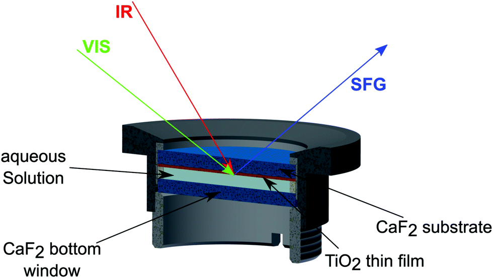Fig. 2 Sketch of the sample cell including the three beams. The IR and the VIS beams travel through the TiO₂ (orange) coated CaF₂ window and hit the interface of the photocatalyst and the D₂O. The SFG signal is detected in reflection mode and also passes the TiO₂ and the CaF₂ before being sent to the detector.

Each spectrum was recorded for 10 min. The raw spectrum was background corrected and normalized to the non-resonant SFG spectrum of a 100 nm gold film also deposited on a CaF₂ window, to correct for the frequency dependence of the IR beam.

For phase-resolved measurements another setup has been used, as described elsewhere.¹⁷

3 Results and discussion

Fig. 3 shows the SFG spectra for D₂O at various pD-values in contact with an 85 nm (a) and a 150 nm (b) thick layer of TiO₂ measured in the OD-stretch vibration region. All spectra show three peaks between 2000 and 2600 cm⁻¹, originating from hydrogen-bonded OD-stretch vibrations. For both layer thicknesses, the spectral intensity varies with the pD in such a way that a minimum at pD 5 (black) can be observed, whereas the intensities rise steadily from 5 to 3 (red) for more acidic and from 5 to 7 (blue), 9 (green) and 11 (pink) for more basic solutions.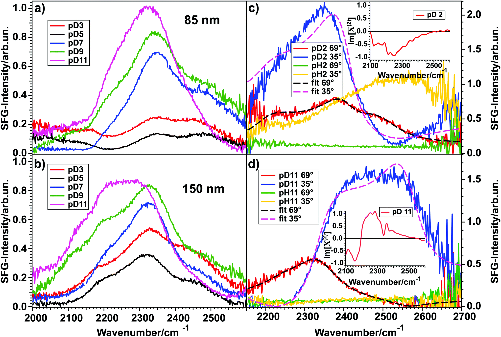

Fig. 3 (a and b) Spectra for pD 3, 5, 7, 9, and 11 in contact with an 85 nm and a 150 nm thick TiO₂ layer, respectively. (c and d) SFG spectra and fits for pH/pD 2 and pH/pD 11, respectively, in contact with another 150 nm thick TiO₂ sample for two different angles of incidence of the VIS beam, illustrating the influence of the NR signal on the spectral shape. The fits assume a Lorentzian lineshape model.²⁰ Insets show phase-resolved spectra.

As a first approximation, the intensity of an SFG-spectrum depends on the molecular order in the studied system. The non-linear process is only allowed in non-centrosymmetric media, which means that the SFG-signal scales with the degree of interfacial molecular order. For the data shown in Fig. 3(a) and (b), this means that for pD 5 the water molecules are aligned the least and that the order increases when the pD is varied in either direction. The quantification of this finding will be discussed below.

These results stand in contrast to previous data presented by Cremer et al.,¹⁶ obtained on very thin (0.9–3.9 nm) TiO₂ on SiO₂ substrates. They have shown that for pH 12, 10, 8, 6, and 4, the SFG-spectrum of the TiO₂–H₂O interface does not differ much from the SiO₂–H₂O interface. For pH 2 they have seen a larger signal than for the SiO₂ surface. From their data, they could also show an intensity minimum between pH 4 and 6 for the TiO₂–H₂O interface. Indeed, the measurement at pH 2 indicates that TiO₂ is present at the interface. The similarities between the TiO₂–water and SiO₂–water spectra observed for all other pH-values might indicate that a major contribution to the signal could come from the SiO₂–H₂O interface. This interface shows also a strong pH-dependence of the intensity of the SFG-signal.²¹

By comparing panels (a) and (b) it is clear that for high pD the spectral shape is largely independent of the TiO₂ sample. However, for pD 3 and 5 the spectra differ significantly for the two samples. By comparing several different 85 nm and 150 nm samples, we conclude that these differences do not originate from the layer thickness itself, since other samples with a 150 nm layer thickness have shown the same spectral shape for pD 3 and pD 5 as the 85 nm sample. Therefore, we attribute the differences to a different non-resonant signal. In general, a non-resonant signal is a contribution to the total SFG-spectrum that is independent of the frequency of the incoming beams. The exact origin of this contribution is rarely known, though it is often considered to be of electronic origin. Since TiO₂ is a semiconductor it is likely that the non-resonant contribution to the signal is influenced by doping or structural defects and varies from sample to sample.

That indeed the non-resonant contribution from TiO₂ has great influence on the SFG-signal is clear from SFG experiments performed with a different angle of incidence for the visible beam. The results are shown in Fig. 3(c) and (d) for pD 2 and 11, respectively. The experiments were performed on a different TiO₂-sample of 150 nm thickness. The red spectrum shows the signal for pD 2 and 11 for the same vis-angle (69° from the surface normal) as for the spectra shown in panels (a) and (b), but from a different sample. The green trace is the non-resonant signal, obtained upon exchanging D₂O with H₂O at the same angle and pD/pH. Upon changing the visible angle of incidence to 35°, the spectral shape of pD 2 and 11 changes dramatically (blue). For pH 2 (c, yellow) also the non-resonant signal changes, whereas it is less influenced for pH 11 (d, yellow). The non-uniform shape of the non-resonant signal of pH 2 at 35° might arise from the proton band of the H₃O⁺ ions present in the acidic solution.²²

In order to understand the influence of the non-resonant signal on the spectral shape, it is necessary to fit the data from Fig. 3(c) and (d). In general, the SFG-intensity can be expressed as:

with I_VIS and I_IR being the intensities of the visible and the infrared beams, χ⁽²⁾_j as the second-order non-linear susceptibility of the resonance j and χ⁽²⁾_NR being the non-resonant response of the system to the incoming fields.

The details of the water–TiO₂-interaction lie in χ⁽²⁾. This factor can be disentangled as:

where A₀ and φ are the amplitude and the phase of the non-resonant signal, respectively. The resonance is described by the amplitude A_j, the frequency ω_j and the width Γ_j for the jth resonance. As eqn (2) has a Lorentzian shape, an SFG-spectrum can be described as the sum of one or more Lorentz-functions.

Using this model, the spectra of pD 2 and 11 for a visible angle of 69° shown in Fig. 3(c) and (d) were fitted with three Lorentzians for the resonant part, which is shown in black dashed lines. Upon only changing the non-resonant amplitude and phase, as well as the resonances’ amplitudes the spectra for 35° (blue) could be described very well (pink, dashed). These data clearly show that the NR-signal has a large effect on the overall lineshape.

By fitting both datasets we obtained the best description for pD 2 with three peaks at 2150, 2378, and 2462 cm⁻¹, having a positive, negative and negative sign in the Im[χ⁽²⁾], respectively. For pD 11 the fit result is a positive, positive and negative sign in the Im[χ⁽²⁾] for the peaks positioned at 2255, 2333, and 2564 cm⁻¹, respectively. The peak assignment is given below.

A positive sign means that the vibrating molecules’ D-atom (more precisely: its transition dipole moment) points towards the semiconductor. This means that for pD 2 most of the water molecules point downwards (with respect to lab frame), away from the TiO₂ layer, whereas for pD 11 most of them point upwards, towards the semiconductor. The insets in Fig. 3(c) and (d) show the phase-resolved SFG-spectra of the TiO₂–water interface, recorded on yet another TiO₂ sample of 150 nm thickness, which confirms the general trend found by the fitting (for more details see below).

To unravel if the three peaks found in the fit originate from three different water ensembles or (partly) from intra- and/or intermolecular coupling, isotopic dilution experiments were performed. For the water–air interface it is well known that intra- and intermolecular coupling results in the splitting of a single peak into two peaks. Diluting the solution isotopically suppresses both coupling mechanisms, so that the pure resonances are obtained.^23,24Fig. 4 shows the spectra for 100% D₂O (red) and isotopically diluted solutions (blue) of pD 2 (top) and pD 11 (bottom) in contact with the same 150 nm thick TiO₂ sample as used for the angle-dependent measurements shown in Fig. 3(c) and (d).

Fig. 4 SFG-spectra of 100% (red) and 50% D₂O (blue) for pD 2 (top) and pD 11 (bottom). Also shown are the respective fits in dashed green and black lines. All measurements were performed on a 150 nm thick TiO₂ layer. In yellow, turquois, purple and pink the pure contribution of each peak is shown.

For 100% D₂O, the spectra were fitted with three peaks, using eqn (2) and the sign combinations obtained before. Subsequently, all parameters were kept constant and only the amplitudes were let run free in order to fit the 50% spectra. To account for possible coupling effects, a fourth peak in the center of two peaks with equal signs was added. Table 1 shows the fitting parameters obtained for all four spectra. The assignment of each individual peak to vibrating water species will be given below.

Table 1 Fitting parameters for 50% and 100% D₂O solutions of pD 2 and 11, using eqn (2). A_j is the amplitude of the Im[χ⁽²⁾]

	pD2 100%	pD2 50%	pD11 100%	pD11 50%
A NR	0.06	0.06	0.04	0.04
ϕ NR	0.45	0.45	2.04	2.04
A 1	5.1	0.8	11.2	7.2
ω 1	2270	2270	2260	2260
Γ 1	150	150	121	121
A 2	−46.4	−8.8	36.9	15.1
ω 2	2393	2393	2340	2340
Γ 2	181	181	149	149
A 3	−30.0	−14.4	−14.8	−11.9
ω 3	2519	2519	2546	2546
Γ 3	187	187	200	200
A 4	—	−14.3	—	—
ω 4	—	2456	—	—
Γ 4	—	200	—	—

---

For the pD 11 case Table 1 shows that the amplitudes A_j (see eqn (2)) for the 50% D₂O spectra are approximately half the amplitudes of the 100% D₂O spectra. For a 50 : 50 mixture of D₂O and H₂O this is an expected outcome if no inter- or intramolecular coupling is involved.

However, in the pD 2 case only the third peak (A₃) has half the amplitude for the 50 : 50 mixture, whereas the first (A₁) and the central peak (A₂) show approximately a quarter of the initial amplitude. Additionally, in order to adequately describe the data for pD 2, a fourth peak had to be introduced, with a frequency between ω₂ and ω₃.

In general, if a signal is involved in inter- or intramolecular coupling, it is possible that it splits into two separate peaks. Upon isotopic dilution the two signals merge into one peak with a frequency between the two, which is attributed to HDO molecules.²⁵ Moreover, the signal amplitude decreases more than linear. For example, for the coupling of two OH-groups, upon isotopic dilution by 50%, the peaks will decrease to a quarter of the amplitude obtained from 100% solutions, due to the suppression of the coupling. This is only possible if the two initial signals have the same amplitude sign. In Table 1 this effect can be seen for the central and the high-frequency peak. For the 50 : 50 mixture of D₂O and H₂O, the amplitude of the peak at 2393 cm⁻¹ (A₂) has dropped to approximately a quarter of the initial value. Additionally, the appearance of the fourth peak at 2456 cm⁻¹, between the central and the third peak, indicates the presence of HDO-molecules.

However, upon isotopic dilution the amplitude of the peak at 2519 cm⁻¹ has dropped only to half of the value for the pure D₂O solution. Therefore it can be concluded that still a contribution of a molecular species resonating at this frequency, overlapping with the Fermi resonance of the actual 2456 cm⁻¹ peak is present. In the case of pD 11 no fourth peak appears, meaning that the coupling is weak.

Using the knowledge of the correct amplitude signs and the coupling relations as determined above, eqn (2) can be used to fit the data shown in Fig. 3(a) and (b), in order to obtain deeper insights into the nature of water at the water–TiO₂ interface in dependence of the solution pD. Fig. 5 shows the results of the amplitude (a, b) and the frequency (c, d) obtained from the fits for the 85 nm and the 150 nm TiO₂ sample, respectively. As explained above, the signs of the amplitudes for the OD-stretch vibrations of water molecules are related to the direction of their dipole moment. A negative amplitude translates for OD to a molecular dipole moment pointing downwards (with respect to lab frame) and therefore away from the TiO₂ interface. For a positive amplitude the dipole moment points upwards in the direction of the semiconductor.

Fig. 5 Top: Amplitude (A_j) of each peak obtained from fitting the SFG-spectra, plotted against the pD for the 85 nm (a) and the 150 nm (b) TiO₂-sample. The sign is chosen to represent the Im[χ⁽²⁾] signal. The central peak changes sign upon crossing the point of zero charge at approximately pD 5. Lines serve as guides to the eye. Bottom: Central frequency of each of the three peaks for (c) 85 and (d) 150 nm TiO₂. The blue bar marks the transition from a positively to a negatively charged surface, in order to stress the possible change of molecular species responsible for each peak.

From Fig. 5 it is immediately apparent that the peak at 2350 cm⁻¹ changes sign when the pzc is crossed, meaning that the water molecules change their orientation from hydrogen atoms pointing downwards to pointing upwards. For the high- and the low-frequency peaks no sign change occurs, and therefore no reorientation can be observed. The origin of the peaks will be discussed below.

By taking a closer look at the two top panels in Fig. 5, showing the peak amplitudes as a function of the solution pD, an overall intensity minimum for pD 5 can be inferred. In order to visualize this intensity trend better for water at the TiO₂–water interface for different pD-values, the fits obtained from the spectra in Fig. 3(a) and (b) can be used. By setting the non-resonant contribution of the fit result to zero, a purely resonant spectrum can be obtained. Fig. 6 shows the square root of the intensity spectrum, integrated between 2000 and 2700 cm⁻¹.

Fig. 6 Intensities of the square root of the resonant part of the SFG-spectra plotted against the pD. Red triangles show the intensities for the 85 nm TiO₂ layer and blue circles for the 150 nm layer. The intensity shows a minimum at pD5 for both samples. Lines serve as guides to the eye.

The results clearly show a minimum intensity for pD 5 for both samples, whereas it rises when the solution becomes more acidic or basic. Therefore it can be concluded that at pD 5 the water molecules are ordered relatively randomly. For the investigated pD-values, the highest intensity, and therefore the most ordered network, appears at around pD 11.

However, in the case of strongly charged interfaces, the higher intensity could also be a result of third-order processes. The charges at the interface result in a DC field reaching into the water and being responsible for the orientation of the water molecules. If this field becomes strong enough it cannot be neglected, and it can interact with the infrared and visible fields to give rise to a third-order response of the water molecules. Therefore, eqn (1) will change to

with E_DC being the strength of the DC field and χ⁽³⁾ being the third-order susceptibility of the water molecules. This process is allowed in centrosymmetric environments and therefore can influence water molecules up to 1 μm away from the interface. This bulk effect can contribute greatly to, or even overwhelm the χ⁽²⁾ signal from the direct interfacial water.²⁶

To check whether the χ⁽³⁾ contribution caused by the strong interfacial charge is significant, its DC field can be screened by adding excess ions into the solution. For positively charged surfaces, negatively charged ions will be attracted towards the interface, shielding the DC field for lower water layers. The result is the suppression of the χ⁽³⁾ contribution to the SFG-signal and therefore a pure χ⁽²⁾ signal originating from the water molecules aligned by the surface charge will be obtained. For negatively charged surfaces the same effect can be observed due to the migration of positively charged ions towards the semiconductor. Fig. 7 shows the spectra recorded for yet another 150 nm thick TiO₂ sample in contact with pD 3 and 11 solutions with NaCl concentrations of 0, 10 and 100 mM. The Debye-lengths for these salt concentrations are 9.5, 3.0 and 1.0 nm, respectively.²⁷ Note that for 0 mM NaCl an ion concentration of 1 mM has to be considered, due to the presence of HCl/NaOH in the acidic and basic solutions. Fig. 7 shows that in the case of pD 3 (top), no major change can be observed upon adding salt, demonstrating that the χ⁽³⁾ contribution is negligible, despite the relatively long Debye length of 9.5 nm. For pD 11 (bottom), upon adding 10 mM NaCl, the signal drops by approximately 30% and remains at that level for the 100 mM solution. When remeasuring the pD 11 solution without additional NaCl, the signal does not recover fully. We attribute this difference to experimental variations in the signal intensity.

Fig. 7 SFG-spectra for another 150 nm TiO₂ sample in contact with pD 3 (top) and 11 (bottom) solutions with various NaCl concentrations. The order of the measurements is shown in the legends, namely 0 (red), 10 (black), 100 (blue) and again 0 mM (green) NaCl.

Analysis of the data using the model of Gonella, et al.²⁷ has shown that for pD 11 the χ⁽³⁾ contribution at 10 mM NaCl is less than 30% of the total SFG-signal. Thus, although the surface is charged at high and low pD, the signal originates mainly from the few interfacial layers directly in contact with TiO₂.²⁶

The two bottom panels of Fig. 5 show the pD-dependence of the frequency for each peak resulting from the fit. They show that the high- (ω₃, green) and the low- (ω₁, red) frequency peaks tend to shift to higher frequencies, whereas the central peak (ω₂, black) slightly shifts to lower frequencies. Taking into account that especially for the 150 nm film ω₂ has the highest amplitude, its slight shift should result in a relatively large shift of the whole spectrum. This shift clearly can be seen in Fig. 3(a) and (b) for both samples.

Both the intensity trends and the spectral shift can be explained by the amphoteric nature of TiO₂. The interfacial protonation state of the semiconductor depends on the solution pD. The material's point of zero charge (pzc) lies at around pD 5. At this pD-value, the protonation and deprotonation reactions occur at the same rate, resulting in a zero net charge of the semiconductor. Therefore, the water molecules will not experience an electric field and are ordered, on average, randomly. With decreasing or increasing solution pD, the TiO₂ surface is increasingly protonated or deprotonated, respectively. In the acidic, protonated case, the resulting positive charge causes the majority of the water molecules, represented by the peak at ∼2350 cm⁻¹, to orient with their deuterium atoms towards the bulk water. For basic solutions the semiconductor is deprotonated and the resulting negative charge orients the majority of the water molecules with the deuterium atoms pointing towards the interface. This means upon crossing the pzc the water molecules flip, as clearly demonstrated by the phase-resolved data – see insets in Fig. 3(c) and (d). The higher the interfacial charge, the larger the degree of average water orientation by the resulting electric field, and the higher the intensity of the SFG-signal.

The peak position in general is determined by the hydrogen bonding strength of the vibrating OD-groups. The stronger the hydrogen bond of an OD-group, the lower the oscillation frequency due to the weakening of the covalent OD-bond. The observation of decreasing frequency with increasing pD for water at the TiO₂–D₂O interface therefore implies stronger hydrogen bonding for high pD values. However, also the appearance of different water species with different hydrogen bonding environments can cause variations in the spectral shape of an SFG-spectrum, due to their oscillation at different frequencies.

To summarize the findings of the peak position and molecular orientation we suggest the following peak assignment: the high-frequency peak, caused by oscillators with a transition dipole moment pointing downwards, accounts for the presence of interfacial TiOD groups, which are relatively isolated, forming weak hydrogen bonds for all measured pD values.^17,28 These water molecules are marked in green as shown in Fig. 8, which illustrates the peak assignment for pD values below, at, and above the pzc of TiO₂.

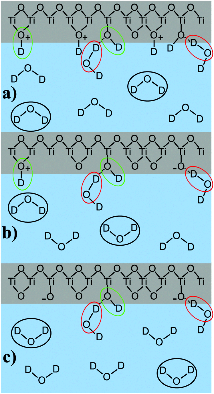Fig. 8 Water orientation in dependence of pD, for the acidic (a), the neutral (pzc at pD 5) (b) and the basic (c) case. Circles indicate the peak (green: high-frequency; black: central frequency; red: low-frequency). For simplicity the counter ions are omitted.

The shift from lower to higher frequencies upon increasing the solution pD could illustrate their even stronger isolation when the pzc is crossed. The isotopic dilution experiments for low pD indicated that parts of this high-frequency peak originate from coupling between the OD stretch mode and the bending overtone, complicating the interpretation of this vibrational mode.

Apart from the mentioned TiOD groups, it is possible that TiOD₂⁺ and bridging Ti–OD⁺–Ti groups also exist in the system.

The low-frequency peak originates from molecules pointing upwards, towards the TiO₂. The low-frequency indicates that these resonators are involved in strong hydrogen bonds. We attribute this peak to water molecules forming hydrogen bonds with the oxygen atom in interfacial TiOD groups, as has been shown before.¹⁷ At high pD, it is also possible that deprotonated TiO⁻ groups are involved in strong hydrogen bonding. This water species is marked red in Fig. 8.

The central peak changes sign upon crossing the point of zero charge. Accordingly, it is assigned to water molecules in underlying layers of D₂O very close to the surface, i.e. most likely in the first two water layers, as the χ⁽³⁾ contribution is very small. These molecules are strongly influenced by the surface charge and marked in black in Fig. 8.

For a protonated, positively charged interface at low pD, the molecules point away from the TiO₂. In the deprotonated case at high pD their deuterium atoms face towards the negatively charged semiconductor. The weak frequency shift allows the assumption that their bonding environment does not change dramatically, meaning that they most probably form hydrogen bonds with other water molecules. As for low pD, this peak is also involved in the coupling with an overtone of the D–O–D bending mode, and its frequency should be considered to be slightly higher than obtained from the fit. In our previous work on anatase TiO₂ this central peak was absent, as that work was performed with water at neutral pH and no additional electrolytes. Thus, the system was close to the point of zero charge.¹⁷

4 Conclusion

The TiO₂–D₂O interface for two different thicknesses of TiO₂ thin films has been probed by SFG spectroscopy for pD values ranging from 3 to 11, showing three peaks for all spectra. The spectral differences seen between different samples are independent of the layer thickness, but rather come from sample to sample variations in the non-resonant background. The spectra show an intensity minimum at pD 5, which is close to the point of zero charge of the semiconductor surface. Upon crossing this value from pD 3 to pD 11, the amplitudes of the peaks lowest and highest in frequency retain their phase, meaning the responsible OD-groups do not change their orientation. Therefore we conclude that for all pD values, and therefore various interfacial charge states, the species responsible for these peaks are the same and that their hydrogen bonding environment does not change significantly. The amplitude of the central peak however changes sign upon crossing the point of zero charge, indicating a flip of this ensemble of water molecules due to the changes in the interfacial charges from positive to negative when the pD of the solution and therefore the protonation state of the semiconductor's surface is changed.

Conflicts of interest

There are no conflicts to declare.

Acknowledgements

The authors would like to thank Hansjörg Menges, Marc-Jan van Zadel, Florian Gericke and Gabriele Hermann for technical support. Special thanks are addressed to Helma Burg for conducting the AFM Measurements in the MPIP. This work was funded by an ERC Starting Grant (no. 336679) and by the Marie Curie Foundation with grant CIG334368. Open Access funding provided by the Max Planck Society.

Notes and references

1. A. Fujishima and K. Honda, Nature, 1972, 238, 37–38.
2. X. Li, J. Yu and M. Jaroniec, Chem. Soc. Rev., 2016, 45, 2603–2636.
3. M. Pelaez, N. Nolan, S. Pillai, M. Seery, P. Falaras, A. Kontos, P. Dunlop, J. Hamilton, J. Byrne, K. O'Shea, M. Entezari and D. Dionysiou, Appl. Catal., B, 2012, 125, 331–349.
4. K. Zhang, Q. Liu, H. Wang, R. Zhang, C. Wu and J. Gong, Small, 2013, 9, 2452–2459.
5. M. Lazzeri, A. Vittadini and A. Selloni, Phys. Rev. B: Condens. Matter Mater. Phys., 2001, 63, 155409.
6. X. Han, Q. Kuang, M. Jin, Z. Xie and L. Zheng, J. Am. Chem. Soc., 2009, 131, 3152–3153.
7. I. Martyanov, S. Uma, S. Rodrigues and K. Klabunde, Chem. Commun., 2004, 2476–2477.
8. A. Arunachalam, S. Dhanapandian, C. Manoharan and G. Sivakumar, Spectrochim. Acta, Part A, 2015, 138, 105–112.
9. P. Fenter and N. Sturchio, Prog. Surf. Sci., 2004, 77, 171–258.
10. M. Ridley, M. Machesky, D. Palmer and D. Wesolowski, Colloids Surf., A, 2002, 204, 295–308.
11. U. Diebold, Surf. Sci. Rep., 2003, 48, 53–229.
12. J. Cheng and M. Sprik, J. Chem. Theory Comput., 2010, 6, 880–889.
13. L.-M. Liu, C. Zhang, G. Thornton and A. Michaelides, Phys. Rev. B: Condens. Matter Mater. Phys., 2010, 82, 161415(R).
14. M. Sumita, C. Hu and Y. Tateyama, J. Phys. Chem. C, 2010, 114, 18529–18537.
15. Y. Shen, Nature, 1989, 337, 519–525.
16. S. Kataoka, M. Gurau, F. Albertorio, M. Holden, S.-M. Lim, R. Yang and P. Cremer, Langmuir, 2004, 20, 1662–1666.
17. S. Hosseinpour, F. Tang, F. Wang, R. Livingstone, S. Schlegel, T. Ohto, M. Bonn, Y. Nagata and E. Backus, J. Phys. Chem. Lett., 2017, 8, 2195–2199.
18. M. Gebhard, L. Mai, L. Banko, F. Mitschker, C. Hoppe, M. Jaritz, D. Kirchheim, C. Zekorn, T. de los Arcos, D. Grochla, R. Dahlmann, G. Grundmeier, P. Awakowicz, A. Ludwig and A. Devi, ACS Appl. Mater. Interfaces, 2018, 10, 7422–7434.
19. M. Gebhard, F. Mitschker, M. Wiesing, I. Giner, B. Torun, T. de los Arcos, P. Awakowicz, G. Grundmeier and A. Devi, J. Mater. Chem. C, 2016, 4, 1057–1065.
20. M. Bonn, Y. Nagata and E. Backus, Angew. Chem., Int. Ed., 2015, 54, 5560–5576.
21. D. Lis, E. Backus, J. Hunger, S. Parekh and M. Bonn, Science, 2014, 344, 1138–1142.
22. L. Levering, M. Sierra-Hernandez and H. Allen, J. Phys. Chem. C, 2007, 111, 8814–8826.
23. J. Schäfer, E. Backus, Y. Nagata and M. Bonn, J. Phys. Chem. Lett., 2016, 4591–4595.
24. M. Sovago, R. Kramer Campen, G. Wurpel, M. Muller, H. Bakker and M. Bonn, Phys. Rev. Lett., 2008, 100, 173901.
25. R. Livingstone, Y. Nagata, M. Bonn and E. Backus, J. Am. Chem. Soc., 2015, 137, 14912–14919.
26. J. Schäfer, G. Gonella, M. Bonn and E. Backus, Phys. Chem. Chem. Phys., 2017, 19, 16875–16880.
27. G. Gonella, C. Lütgebaucks, A. De Beer and S. Roke, J. Phys. Chem. C, 2016, 120, 9165–9173.
28. R. Khatib, E. Backus, M. Bonn, M.-J. Perez-Haro, M.-P. Gaigeot and M. Sulpizi, Sci. Rep., 2016, 6, 24287.

---

Footnotes

† Present address: Institute of Particle Technology (LFG), Friedrich-Alexander-Universität Erlangen-Nürnberg (FAU), Cauerstrasse 4, 91058 Erlangen, Germany.

‡ Present address: Argonne National Laboratory, 9700 South Cass Avenue, IL 60439, USA.

---