A unified theory of weak-field coherent control of the behavior of a resonance state

Abstract

A unified weak-field control scheme to modify the two properties that determine the whole behavior of a resonance state, namely the lifetime and the asymptotic fragment distribution produced upon resonance decay, is proposed. Control is exerted through quantum interference induced between overlapping resonances of the system, by exciting two different energies at which the resonances overlap. The scheme applies a laser field consisting of a first pulse that excites the energy of the resonance to be controlled, and two additional pulses that excite another different energy to induce interference, with a delay time with respect to the first pulse. Each of the two additional pulses is used to control one of the two resonance properties, by adjusting its corresponding delay time: with a relatively short delay time the second pulse controls the resonance lifetime, while with a very long delay time the third pulse modifies the asymptotic fragment distribution produced. The efficiency of the control of each resonance property is found to be strongly dependent on the choice of the second interfering energy, which allows for a more flexible control optimization by choosing a different energy for each property. The theory underlying the interference mechanism of the control scheme is developed and presented, and is applied to analyze and explain the results obtained. The present scheme thus appears to be a useful tool for controlling resonance-mediated molecular processes.

---

1. Introduction

Resonance states govern a large variety of molecular processes that occur upon resonance decay.^1,2 Among them are photodissociation processes like electronic,³ vibrational,^4,5 and rotational⁶ predissociation of a molecular system, as well as low-temperature reactive^7–13 and nonreactive^14–21 molecular collisions. Control of such molecular processes has been actively pursued in the last few decades.^22–34 In the case of resonance-mediated processes, their control is closely related to the control of the underlying resonance decay process. And the behavior of this decay process is determined essentially by two resonance properties which are the lifetime (which determines the duration of the process) and the product fragment state distribution produced upon the decay (which determines the outcome of the process). Thus, modifying these resonance properties provides an effective means of control over the resonance-mediated process of interest.

Strategies to control the resonance lifetime based on quantum interference have been suggested in environments of both overlapping and isolated resonance states in the weak-field regime.^35–39 Quantum interference was also the basis of different weak-field control schemes proposed to modify the fragment distribution produced upon resonance decay.^40–44 Some of the above control schemes share the common feature that they apply a pump laser field consisting of two pulses with a time delay between them.^{36,37,39,42–44} Each of these two pulses is used to excite a different resonance energy in an environment of overlapping resonances, which then interfere. By varying the time delay between the pulses, the resonance interference can be controlled. Depending on how long is the time delay between the pulses, control of a different resonance property (either the lifetime or the fragment distribution) is achieved. More specifically, if the time delay between the pulses is relatively short, such that the two resonances are simultaneously populated in time, the lifetime of both resonances can be controlled.^36,37,39 However, when the time delay is long enough such that the population of the resonance excited with the first pulse has decayed completely when the other resonance is excited with the second pulse, then the product fragment distribution associated with the first resonance can be modified in the asymptotic time regime.⁴⁴ Thus, the time delay applied between pulses is related to the nature and time scale of the resonance property under control.

So far the above type of control scheme has been applied to modify separately either the resonance lifetime or the fragment distribution. However, it is possible – and desirable – to design a unified control scheme that allows for the control of the two resonance properties determining the behavior of a resonance-mediated molecular process. Indeed this can be done by applying a laser field consisting of several pulses, where the first pulse would excite the resonance to be controlled, while the subsequent pulses would be delayed with respect to the first one accordingly to the dynamical time scale of the resonance property which is to be modified. The practical advantage of such a unified scheme is that the behavior along the whole course of the process of interest can be controlled within a single experiment, just by choosing appropriately the time delay of the pulses that control each resonance property. The main goal of the present work is to demonstrate the possibility of this unified control scheme both numerically and formally, by developing the underlying equations of the theory. As in earlier works the scheme is applied to the vibrational predissociation of the Ne–Br₂(B,ν′) complex, because this system features overlapping resonances in different regimes. Resonances are common to several types of weakly bound complexes.⁴⁵

This paper is organized as follows. Section 2 presents the main features of the methodology applied, and the formal theory underlying the control scheme. In Section 3 the results are presented and discussed. Conclusions are given in Section 4.

2. Theory

Upon laser excitation, Ne–Br₂(X, ν′′ = 0) + hν → Ne–Br₂(B,ν′,n′), an intermolecular van der Waals resonance n′ of Ne–Br₂(B,ν′) is populated. The labels ν′′ and ν′ denote the vibrational states of Br₂ in the X and B electronic states, respectively, while the n′ index labels the energy position of the resonance, with n′ = 0 corresponding to the ground one. Then the resonance excited decays to the fragmentation continuum through vibrational predissociation, Ne–Br₂(B,ν′,n′) → Ne + Br₂(B, ν_f < ν′). This process has been studied in detail both experimentally^46,47 and theoretically.^4,5

The Ne–Br₂(B,ν′,n′) excitation with a laser field and the subsequent predissociation were simulated with a full three-dimensional wave packet method (assuming J = 0) described in detail elsewhere.^4,35 In order to assess the quality of the model applied, it is noted that the lifetime calculated with the present theoretical model for the decay of the Ne–Br₂(B, ν′ = 16) ground intermolecular resonance was found to be 69 ps,³⁸ while the corresponding lifetime estimated experimentally is 68 ± 3 ps.⁴⁷ This good agreement implies that both the three-dimensional wave packet method and the potential surfaces used in the present simulations are realistic enough in order to describe this resonance decay process.

In what follows the formal theory underlying the unified control scheme proposed in this work is developed. Let Ĥ be the total Hamiltonian of a molecular system that supports resonances. Following the discussion on the decay of a resonance state of Cohen-Tannoudji et al.,⁴⁸ we can write Ĥ as Ĥ = Ĥ₀ + W, where Ĥ₀ is a zeroth-order Hamiltonian and W is a coupling. The spectrum of Ĥ₀ consists of a set of discrete bound states χ_i (located in the interaction region) with associated energies E_i, and a set of continuum states φ_E,m (associated with the product fragments in the asymptotic region) with associated energies E and with m a global label for the fragment internal states. When W = 0 the χ_i states are true bound states, but when W ≠ 0, χ_i become resonances ψ_i that decay to the continuum of φ_E,m states. These states fulfill the orthogonality relations

〈χ_i|χ_j〉 = δ_ij, 〈φ_E′,m′|φ_E,m〉 = δ_m′mδ(E′ − E), 〈χ_i|φ_E,m〉 = 0 (1)

and form a complete basis set, in terms of which the state of the system excited at the energy E can be expressed. Let ψ_E be the stationary eigenstates of Hamiltonian Ĥ associated with energy E in the excited electronic state. Such eigenstates (which also form a complete basis set) can be expanded in the set of the χ_i and φ_E,m states aswhere the above summation over k considers the possibility that in general more than one state χ_k may contribute to ψ_E(t) in an environment of overlapping resonances. The time dependence of ψ_E(t) is the trivial one (i.e., |ψ_E(t)|² is time independent, as can be easily checked by applying the relations of eqn (1)).

Let us now assume that within a vibrational manifold ν′ of Ne–Br₂(B,ν′) featuring a group of intermolecular overlapping resonances, a given resonance energy E_a is excited with an electric field consisting of a Gaussian-shaped pulse, 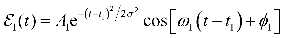, where A₁ is the pulse amplitude, t₁ is the time center of the pulse, σ is related to the pulse temporal width, ω₁ is the photon frequency required to excite the resonance energy E_a from the ground vibronic state Ne–Br₂ (X, ν′′ = 0, n′′ = 0), and ϕ₁ is the pulse phase. It is noted that in a framework of overlapping resonances, several resonances may contribute at a given energy E_a, one of them providing the dominant contribution.⁴⁹ Excitation of the system by creates a wave packet ξ_Ea(t) that can be expressed as

where and . The basis of the control scheme suggested is to induce quantum interference between the overlapping resonances, and to achieve this goal (at least) two resonance energies are to be excited by applying a laser field with two Gaussian pulses,where ω₁ and ω₂ are the pulse frequencies corresponding to the excitation of the two resonance energies, and Δt = t₂ − t₁ is the delay time between the two pulses. When the laser field is applied to excite the resonance energies E_a (excited by the pulse centered at t₁) and E_b (excited by the pulse centered at t₂), a wave packet is created,

Φ(t) = ξ_Ea(t) + ξ_Eb(t), (5)

with ξ_Ea(t) and ξ_Eb(t) being the amplitudes excited around E_a and E_b by the two pulses of . We shall assume that the two pulses of are spectrally narrow enough such that they, and therefore ξ_Ea(t) and ξ_Eb(t), do not overlap in energy. Now, using eqn (3) we can write,

2.1 Control of the resonance lifetime

As discussed in earlier works,^35–39 control of the resonance lifetime is achieved by modifying the shape of the resonance survival probability by means of quantum interference. A resonance wave function ψ_i can be expressed asIf the target resonance for which we want to control the lifetime is that associated with energy E_a, by using eqn (6) and (7) we can express its survival probability I_a(t) aswhere and .

Eqn (8) shows that I_a(t) consists of four terms. The first term, , is the survival probability that would be obtained if a single resonance energy E_a was excited with the field. The lifetime associated with this survival probability would be the “isolated resonance lifetime”, τ^iso_a. The three additional terms of eqn (8) arise from the excitation of amplitude at the second energy E_b and its interference with the resonance amplitude excited at E_a. Those three terms are nonzero as long as the and amplitude coefficients are simultaneously nonzero. Such a condition is fulfilled if the two energies are excited simultaneously, which is achieved if the two pulses of overlap in a temporal range. The effect of these interference terms is “dressing” the isolated resonance survival probability , and therefore changing its shape. As a result of this change in shape, the lifetime associated with I_a(t) also changes from τ^iso_a to a different value. By varying the delay time Δt between the pulses, one can modify the range of temporal overlap between them, and therefore the relative magnitude of the and amplitudes excited simultaneously. This causes variation of the interference terms in a controlled manner, which leads to a change in the shape of I_a(t) and to the control of the associated lifetime.

As shown by eqn (8), the basis of the resonance lifetime control is the quantum interference between resonance amplitudes generated simultaneously in the interaction region of Ĥ by different pulses of the laser field applied, with a delay time between them. Clearly, this interference is not possible if the amplitudes are not generated at the same time, and the interference effect vanishes when the resonance population decays completely. Thus the requirement of simultaneous population of the interfering amplitudes implies a temporal overlap of the pulses to a certain extent, which means that the delay time between them must be smaller than the sum of their half temporal widths. It is noted from the above equations that the quantum interference on which the control effect is based does not require particularly high amplitudes of the pulses (A₁ and A₂), which allows application of the control scheme under weak-field consditions.

2.2 Control of the asymptotic fragment state distribution

The fragment state distribution produced upon resonance decay is the other property that determines the outcome of a resonance-mediated molecular process. The final fragment distribution of a molecular system at a given energy E is determined by the asymptotic behavior – in the region of separated fragments – of the corresponding stationary eigenfunction ψ_E, which is an intrinsic property of Ĥ. However, despite this intrinsic character, it is also possible to modify and control the energy-resolved asymptotic fragment distribution produced upon resonance decay by means of quantum interference in the weak-field regime, as shown in the following.⁴⁴

The asymptotic probability of the fragment state φ_E,m at energy E can be expressed as

where is a constant and Φ(t) is the wave packet created by the electric field applied. Let us suppose now that we want to control the energy-resolved asymptotic fragment distribution produced upon decay of the resonance associated with energy E_a. To achieve this goal by quantum interference we again apply the two-pulse laser field of eqn (4), that excites the same two resonance energies E_a and E_b, and thus creates a wave packet Φ(t) like that of eqn (5). The only difference with the previous situation of the control of the resonance lifetime is that now the delay time Δt = t₂ − t₁ between the two pulses is very long. The reason for the long delay time of the second pulse exciting the E_b energy with respect to the first one is to allow enough time for the first resonance excited at E_a to decay completely and to reach the asymptotic time regime of the fragment distribution produced. Then, by using the expression of Φ(t) of eqn (6), where the asymptotic fragment states φ_Ea,m have been populated after the decay of the population excited to E_a, we can project out Φ(t) onto the fragment states φ_Ea,m to calculate the distribution at energy E_a,where eqn (1) were used. The product state distribution at a time t long enough finally becomes

Eqn (11) is very similar to eqn (8) in that it also consists of a sum of four terms, three of which arise from the excitation of both the E_a and E_b energies and the interference between them. If a single-pulse field is applied to excite E_a, then ξ_Ea(t) ≠ 0, ξ_Eb(t) = 0, and the distribution becomes , where interference is absent. Excitation of the second energy E_b by applying induces interference between the overlapping resonances which manifests itself in the three additional terms of eqn (11). It is stressed that the interference terms of eqn (11) will appear as long as the amplitude ξ_Eb(t) is created by the second pulse of , and this can be done at any asymptotic time as long as desired, and as many times as desired (using further successive pulses after the second one in the laser field).⁴⁴

The mechanism of interference between amplitudes produced in continuum fragment states by exciting two overlapping resonances with a long delay time between the two excitations may appear somewhat ellusive. It can be described as follows. Initially the first pulse of excites the resonance energy E_a creating the ξ_Ea(t) wave packet amplitude. After a long time, once this amplitude has decayed completely to the continuum states and has reached the asymptotic behavior, the second pulse of excites the resonance energy E_b creating the ξ_Eb(t) amplitude. Since both resonances overlap they share common continuum states φ_E′,m′ in a range of energies E′. The second pulse initially populates the χ_k states in the interaction region with an amplitude . After some time this amplitude decays to the continuum states φ_E′,m′, spreading and redistributing temporarily among those φ_E′,m′ states which are shared by both ξ_Ea and ξ_Eb, producing the amplitude . The appearance of this amplitude is what causes interference with the “asymptotic” amplitude generated much earlier by the decay of the resonance amplitude excited by the first pulse. The amplitude , however, is generated in the φ_Ea,m states only temporarily, during the time that the second delayed pulse excites amplitude to E_b that will further decay initially to φ_Ea,m states shared with ξ_Ea. After the second pulse is over all the amplitude temporarily generated in φ_Ea,m states vanishes, redistributing among φ_Eb,m states that contribute to the asymptotic distribution P_m(E_b,t_∞), because the amplitude excited at E_b cannot contribute to the asymptotic E_a distribution P_m(E_a,t_∞). As a result, the interference effect ceases, and P_m(E_a,t_∞) converges to . This is the expected result, in agreement with the previous prediction⁵⁰ that no permanent weak-field coherent control of fragment distributions is possible after the excitation pulse has vanished.

The weak-field strategy applied to control the fragment distribution and reflected in the interference of eqn (11) has similarities with that used in strong-field control techniques. Indeed, the second pulse of plays a similar role as the control field in strong-field techniques, in the sense that it produces the desired control effect while it is on. The difference is that the control effect on the fragment distribution ceases when the control pulse is over in the present weak-field scheme, while it remains in the strong-field case. This, however, does not prevent an effective control of the fragment distribution in the case of the weak-field scheme, if the fragments are detected or moved to other vibronic states of interest (applying a further laser pulse) while the interference effect takes place.

The origin and the basis of the interference in eqn (8) and (11), which govern the control of the resonance lifetime and the fragment diistribution, respectively, are essentially the same, and they only differ in the magnitude of the delay time between the pulses exciting E_a and E_b (relatively short in the case of the lifetime, and very long, in the asymptotic time regime for the fragment distribution). This common origin of the interference effect allows one to design a unified, single control scheme for the two resonance properties. Indeed, a simple way to control both the lifetime and the fragment distribution using a single scheme is to apply two “control pulses”, with a different delay time, with each of these pulses controlling one of the two resonance properties. More specifically, the electric field applied would consist of a combination of three Gaussian pulses,

where the first pulse centered at t₁ would excite the energy E_a of the resonance for which we want to control the lifetime and the fragment distribution, creating the amplitude ξ_Ea; the second pulse centered at t₂ would excite the energy E_b generating the amplitude ξ_Eb with a delay Δt₁₂ = t₂ − t₁ relatively short so as to overlap in time with the first pulse, thus allowing for the control of the resonance lifetime; and the third pulse centered at t₃ would also excite the energy E_b creating , but now with a very long delay Δt₁₃ = t₃ − t₁ which allows for the control of the fragment distribution following eqn (11). In the simulations t₁ is fixed at t₁ = 0, which implies that Δt₁₂ = t₂ and Δt₁₃ = t₃. Thus, application of a single electric field makes possible the control of the two resonance properties that govern a molecular process by just using the appropriate delay time between the different pulses involved in the field.

A few remarks on the above control scheme are now due. In the previous discussion of the equations we have restricted to the excitation of the resonance energies (i.e., the energy of the resonance lineshape peak) for E_a and E_b. However, this is not a requirement of the scheme, and any other energies E_a and E_b different from the resonance ones can be excited, as long as the resonances involved overlap at those energies. The only avantage of exciting the resonance energies is that the control scheme becomes more efficient in principle, because the amplitude generated at the lineshape peaks associated with E_a and E_b is maximized (then maximizing the intensity of interference) with respect to other pairs of energies. For simplicity of the above description excitation of only two energies has been considered. But in the scheme the number of energies excited is not restricted, and excitation of more than two energies also increases the efficiency of the interference effect for the control of both the lifetime³⁷ and the fragment distribution.⁴⁴ All the above indicates that the applicability of the control scheme is quite flexible and general.

3. Results and discussion

In order to illustrate how the unified control scheme works, the simulations will focus on the excitation of the Ne–Br₂(B, ν′, n′ = 0) ground intermolecular resonance in two different situations, namely ν′ = 27 and ν′ = 35. The essential difference between them is that the resonances overlap more strongly in the case of ν′ = 35. Regarding the specific parameters of the field applied in the simulations, for simplicity it is assumed that ϕ₁ = ϕ₂ = ϕ₃ = 0. The amplitudes are A₁ = A₂ = 1.0 × 10⁻⁶ a.u., and A₃ = 3.0 × 10⁻⁶ a.u. in the case of ν′ = 27, while for ν′ = 35 the values are A₁ = A₂ = 1.0 × 10⁻⁶ a.u., and A₃ = 2.0 × 10⁻⁶ a.u. All these amplitudes correspond to a maximum pulse intensity of the order of 10⁴ W cm⁻², within the weak-field regime. The same full width at half maximum, FWHM = 200 ps (related to σ), is used for all the pulses in the different simulations. With this temporal width the corresponding spectral profiles of the pulses of are narrow and do not overlap.

Two electric fields are applied in the simulations, namely and , in order to compare the results obtained for both the resonance lifetime and the fragment distribution in the situations of the absence of interference when exciting a single energy, and when two interfering energies are excited. In both cases the survival probability associated with the ground intermolecular resonance of either the ν′ = 27 or ν′ = 35 vibrational manifolds is calculated according to eqn (8) as I_k=0(t) = |〈ψ_k=0|Φ(t)〉|², where ψ_k=0 is the wave function associated with the ground resonance, and Φ(t) is the wave packet prepared by the electric field applied. Now the corresponding lifetime, τ, is obtained by fitting I_k=0(t) to the function

CC(t) being the cross-correlation function of the laser field or and A an amplitude scaling parameter.

The energy-resolved product fragment state distribution is calculated as follows. In the simulations the wave packet is represented in Jacobian coordinates (R,r,θ), where R is the distance between the Ne atom and the Br₂ center of mass, r is the Br–Br internuclear distance, and θ is the angle between the vectors associated with R and r. In this representation the rovibrational eigenstates associated with the Br₂(B,v,j) fragment are ζ^(j)_v(r)P_j(cos θ), where ζ^(j)_v(r) are the vibrational eigenfunctions of Br₂(B) with associated energies E_v,j and P_j(cos θ) are Legendre polynomials, v and j being the Br₂ vibrational and rotational quantum numbers, respectively. The population of the Br₂(B,v,j) fragment states is computed along time by projecting out the wave packet onto the corresponding states

where C is a constant factor, R_c is a suitably large distance of the dissociation coordinate R, E is the total energy of the system, and k_v,j is given by

k_v,j = [2μ_Br2(E − E_v,j)]^1/2, (15)

with μ_Br2 being the Br₂ reduced mass. The population in each vibrational state of Br₂(B,v) is now calculated as

In the first set of simulations the Ne–Br₂(B, ν′ = 27, n′ = 0) ground intermolecular resonance is excited. As shown in the associated excitation spectrum (Fig. 1), this resonance overlaps with some orbiting resonances of Ne–Br₂(B, ν = ν′ − 1 = 26).^5,35 The main peak of the spectrum located at E_a = −61.8 cm⁻¹ corresponds to the Ne–Br₂(B, ν′ = 27, n′ = 0) ground resonance, while the peak at E_b = −60.63 cm⁻¹ and a weak peak at E = −59.5 cm⁻¹ correspond to two v = 26 orbiting resonances overlapping with each other and with the ν′ = 27 ground resonance. The spectral profiles of the three pulses of (A₁ = A₂, A₃ = 3A₁; the first pulse of coincides with that of ) are plotted in Fig. 1. As shown in the figure, there is no spectral overlap between the first pulse of and the other two.

Fig. 1 Excitation spectrum of the Ne–Br₂(B, ν′ = 27) ground intermolecular resonance. The energies E_a = −61.8 cm⁻¹ and E_b = −60.63 cm⁻¹ (relative to the Ne + Br₂(B, ν′ = 27, j′ = 0) dissociation threshold) of the two overlapping resonances excited by the laser fields are indicated in the figure. Two additional energies E_b = −60.85 cm⁻¹ and E_b = −61.12 cm⁻¹ used in the simulations are indicated by arrows. The spectral profiles of the pulses used in the and fields to excite the E_a and E_b energies are also shown.

As discussed above, when the single-pulse field is applied to excite only the energy E_a, there is no possibility of interference and the asymptotic fragment distribution becomes . In the case of Ne–Br₂(B, ν′ = 27), when the energy E_a = −61.8 cm⁻¹ is excited by , the energy-resolved Br₂(B,v_f) vibrational distribution associated with E_a, calculated with eqn (14)–(16), is shown in Fig. 2. The population distributes among four vibrational final states, ν_f = ν′ − 1, ν′ − 2, ν′ − 3, and ν′ − 4, and these populations reach their asymptotic, constant values for t > 1000 ps.

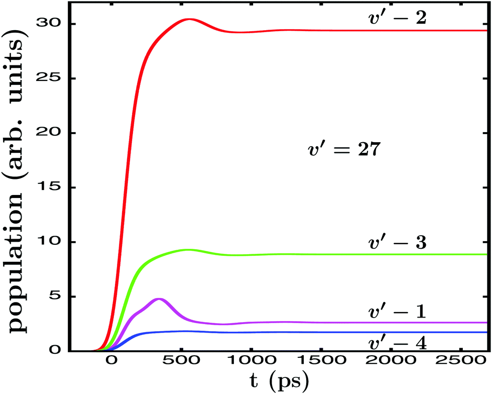Fig. 2 Energy-resolved Br₂(B,v_f) fragment populations in the ν_f = ν′ − 1,…, ν′ − 4 final vibrational state, upon predissociation of Ne–Br₂(B, ν′ = 27) when the E_a −61.8 cm⁻¹ energy is excited by the single-pulse field.

Now, in order to exert control on both the Ne–Br₂(B, ν′ = 27) ground resonance lifetime and the associated fragment distribution, the field of eqn (12) is applied. The first and second pulses (centered at t₁ and t₂, respectively) excite the E_a and E_b energies, respectively, with a delay time Δt₁₂ = 160 ps. The reason for choosing this specific delay time Δt₁₂ is because it was previously shown that it maximizes the lifetime of the Ne–Br₂(B, ν′ = 27) ground resonance.³⁶ With such a delay time the first and second pulses of overlap in time to some extent, as shown by the temporal profile of Fig. 3(a). The next step is the modification of the Br₂(B,v_f) fragment vibrational distribution, by applying the third pulse (centered at t₃) of to excite again the E_b energy, but with a long delay time Δt₁₃ within the asymptotic time region t > 1000 ps of the distribution. Specifically, two values Δt₁₃ = 1500 and 2200 ps have been chosen. The reason for using two different Δt₁₃ values instead of only one is to illustrate the fact that the interference effect can be induced in the asymptotic fragment distribution as many times as desired, as discussed above. The whole temporal profiles of the fields applied with the two Δt₁₃ delays are shown in Fig. 3(a).

Fig. 3 (a) Temporal profile of the laser field applied in the case of Ne–Br₂(B, ν′ = 27). While Δt₁₂ = 160 ps, two situations are shown where the delay time Δt₁₃ = t₃ − t₁ of the third pulse of takes two different values, namely Δt₁₃ = 1500 and 2200 ps. (b) Survival probability of the Ne–Br₂(B, ν′ = 27) ground intermolecular resonance calculated when the single-pulse and the electric fields are applied. (c) Energy-resolved Br₂(B,v_f) fragment vibrational populations in the ν_f = ν′ − 1,…, ν′ − 4 final vibrational state associated with the E_a = −61.8 cm⁻¹ energy, produced upon predissociation of Ne–Br₂(B, ν′ = 27) when the field is applied, with two delay times, Δt₁₃ = 1500 and 2200 ps, between the first and third pulses of . The energy E_b = −60.85 cm⁻¹ is excited by .

The survival probability of the Ne–Br₂(B, ν′ = 27) ground resonance, I_k=0(t), calculated when the single-pulse field and the fields of Fig. 3(a) are applied are displayed in Fig. 3(b). When is used, displays the shape of the convolution of the Gaussian pulse cross-correlation curve with the exponential decay associated with a single resonance, reflected by eqn (13). By fitting I_k=0(t) with eqn (13) the associated lifetime τ^iso_k=0 = 23.5 ps is obtained.³⁶ By applying the E_a and E_b energies are excited by the first two pulses, and they interfere. This interference manifests itself in pronounced undulations in I_k=0(t) in the time range where the two interfering resonances remain populated. This is the interference effect reflected by eqn (8). As previously shown,³⁶ those undulations are separated by a constant time interval which is the inverse of the energy difference E_b − E_a. By fitting now this I_k=0(t) function with eqn (13) a lifetime τ_k=0 = 75 ps is obtained.³⁶ Thus an enhancement of the resonance lifetime by a factor of three can be achieved by means of quantum interference. The survival probability of Fig. 3(b) shows that when the third pulse of is applied to excite E_b with the two Δt₁₃ delays, the ground resonance is populated again, which is the behavior expected for resonances that overlap at different energies, among them E_b.

The Br₂(B, ν_f < ν′) fragment distributions obtained when the fields of Fig. 3(a) are applied are shown in Fig. 3(c). A clear modification of the asymptotic vibrational populations is induced when the third pulse of excites the E_b energy at the two Δt₁₃ delays, as previously found.⁴⁴ During the application of the third pulse the populations display some undulations that reflect the interference effect predicted by eqn (11). As discussed above, once the third pulse is over and the resonance excited at E_b has decayed completely, the asymptotic populations converge back to the values of the populations of Fig. 2. The interference effect is increasingly more intense as the vibrational population is larger in magnitude, because the larger is the amplitude the larger will be the interference terms of eqn (11). In this sense it is noted that the second pulse of also causes an interference effect on the vibrational populations of Fig. 3(c) around Δt₁₂ = 160 ps, although much weaker since A₂ = A₃/3.

The results of Fig. 3 provide a practical illustration of the predictions of eqn (8) and (11). They demostrate that it is indeed possible to design a unified control scheme to modify the two resonance properties, namely the lifetime and the fragment distribution produced upon resonance decay, which govern a resonance-mediated molecular process. The above fact remains valid when we move to a stronger overlapping regime, as shown in the following.

The excitation spectrum associated with the Ne–Br₂(B, ν′ = 35, n′ = 0) ground intermolecular resonance is shown in Fig. 4. It displays a stronger, more congested overlapping regime between different intermolecular resonances. The main peak of the spectrum, located at energy E_a = −56.34 cm⁻¹, corresponds to the ν′ = 35 ground resonance. This resonance lies below the Ne + Br₂(B, ν′ − 1 = 34, j′ = 0) dissociation threshold, and therefore it is embedded in the spectrum of intermolecular resonances of the ν′ − 1 = 34 vibrational manifold, which allows the remaining features of the spectrum of Fig. 4 to originate.⁵¹ Those resonances are broad enough so as to produce a stronger overlapping regime than in the case of Ne–Br₂(B, ν′ = 27).

Fig. 4 Excitation spectrum of the Ne–Br₂(B, ν′ = 35) ground intermolecular resonance. The energies E_a = −56.34 cm⁻¹ and E_b = −57.75 cm⁻¹ (relative to the Ne + Br₂(B, ν′ = 35, j′ = 0) dissociation threshold) excited by the laser fields are indicated in the figure. Two additional energies E_b = −57.10 cm⁻¹ and E_b = −60.76 cm⁻¹ used in the simulations are indicated by arrows. The spectral profiles of the pulses used in the and fields to excite the E_a and E_b energies are also shown.

In a first simulation the energy E_b of the spectrum of Fig. 4 chosen to induce interference is E_b = −57.75 cm⁻¹. While in a strong overlapping regime like that of Fig. 4 several resonances of the ν′ − 1 = 34 manifold (along with the ground resonance of ν′ = 35) overlap at this energy, it was previously determined that among them the dominant resonance is n = 9. The same as in Fig. 1, the spectral profiles of the three pulses of (A₁ = A₂, A₃ = 2A₁) are plotted in Fig. 4.

In the case of the control of the behavior of the Ne–Br₂(B, ν′ = 35) ground resonance, an laser field with a Δt₁₂ = 120 ps delay time has been applied (see Fig. 5(a)). As found previously,³⁹ this is the delay time that maximizes the enhancement of the ν′ = 35 ground resonance lifetime. As in the previous case of Ne–Br₂(B, ν′ = 27), the same Δt₁₃ delays, namely Δt₁₃ = 1500 and 2200 ps, are used.

Fig. 5 The same as Fig. 3 but for Ne–Br₂(B, ν′ = 35), with E_a = −56.34 cm⁻¹ and E_b = −57.75 cm⁻¹.

The survival probabilities associated with the Ne–Br₂ (B, ν′ = 35, n′ = 0) resonance when the and fields are applied are shown in Fig. 5(b). A qualitatively similar interference pattern to that of Fig. 3(b) is found in I_k=0(t) when the field is applied, as compared to the plain survival probability curve obtained with . However, the intensity of interference and the change of the shape of I_k=0(t) appear to be more pronounced in the present case than for ν′ = 27. Actually, the τ^iso_k=0 lifetime associated with the survival probability obtained with is τ^iso_k=0 = 3.8 ps, while the lifetime found when applying is τ_k=0 = 61.0 ps.^37,39 Thus the ν′ = 35 ground resonance lifetime is enhanced by a factor of 15, compared to the factor of 3 obtained for ν′ = 27. This larger effect of interference in the lifetime enhancement is likely due to the stronger overlapping between the n′ = 0 and the n = 9 resonances compared to the ν′ = 27 situation of Fig. 1. As discussed below, this result is related to the magnitude of the coefficients and of eqn (8), which depend on the intensity of the excitation spectrum at E_a and E_b, which is expected to be higher for stronger resonance overlap. As the overlap between the resonances increases, the magnitude of the amplitudes and in eqn (8) increases as well, producing a more intense interference effect. This is supported by the result that when the pair of resonances excited is n′ = 0 and n = 7 (located at −60.76 cm⁻¹ in the spectrum of Fig. 4), with a weaker overlap than n′ = 0 and n = 9, τ_k=0 was enhanced only up to τ_k=0 = 37.0 ps under the same laser field conditions, i.e., somewhat more than half the enhancement achieved with the n′ = 0 and n = 9 resonances.³⁹ Thus the main effect of increasing the intensity of resonance overlap would be to enhance the degree of control of the resonance lifetime.

The energy-resolved Br₂(B, ν_f < ν′ = 35) fragment distributions obtained by applying the fields of Fig. 5(a) are displayed in Fig. 5(c). Since the Ne–Br₂(B, ν′ = 35, n′ = 0) resonance lies below the Ne + Br₂(B, ν′ − 1 = 34, j′ = 0) dissociation threshold, the ν′ − 1 dissociation channel is closed, and the only open channels are ν_f ≤ ν′ − 2. For ν′ = 35 there are twice the number of open channels than for ν′ = 27. The vibrational populations reach their asymptotic, constant values for t > 500 ps. The interesting result is that a similar interference effect to that of the distributions of Fig. 3(c) is found in the present distributions when the third pulse of is applied. So again the same qualitative interference behavior is found regardless of the intensity of resonance overlap. In Fig. 5(c) the intensity of the interference effect is somewhat weaker than in Fig. 3(c), which is not surprising since now A₂ = 2A₁, while for ν′ = 27 A₂ = 3A₁. However, the same as with the resonance lifetime, the stronger resonance overlap is also expected to favor the intensity of interference in the asymptotic fragment distribution. Indeed, again related to the and coefficients of eqn (6), the interfering amplitudes and of eqn (11) will be correspondingly larger for a stronger resonance overlap.

3.1 Dependence of the control of the E_b energy

In the results of Fig. 3 and 5 discussed so far both the E_a and E_b energies chosen to interfere coincide with resonance energies. As commented above, this is not a requirement of the control scheme, and control is also achieved if different energies are excited by the pump laser field. In fact, exciting E_b energies different from the resonance ones E_b = −60.63 cm⁻¹ (for ν′ = 27) and E_b = −57.75 cm⁻¹ (for ν′ = 35) illustrates very nicely how the control scheme operates. In this sense, simulations exciting two additional E_b energies different from E_b = −60.63 cm⁻¹ or E_b = −57.75 cm⁻¹ in the cases of ν′ = 27 and ν′ = 35, respectively, have been carried out. More specifically, the simulations apply the same laser fields of Fig. 3(a) and 5(a), exciting the same E_a resonance energies as before (i.e., E_a = 61.8 cm⁻¹ for ν′ = 27 and E_a = 56.34 cm⁻¹ for ν′ = 35), but now changing E_b to values of 61.12 and 60.85 cm⁻¹ for ν′ = 27, and 57.10 and 60.76 cm⁻¹ for ν′ = 35. The additional E_b energies excited are indicated by arrows in Fig. 1 and 4 for ν′ = 27 and 35, respectively. Survival probabilities and energy-resolved Br₂(B,v_f) fragment distributions are calculated with the new E_b energies, and they are compared in Fig. 6 and 7 with those shown in Fig. 3 and 5.

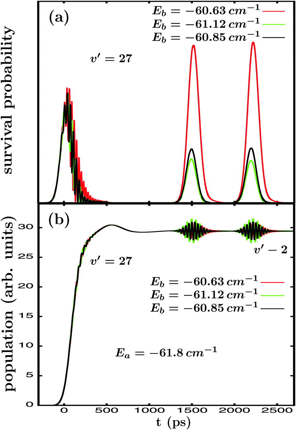Fig. 6 Comparison of the (a) survival probabilities of the Ne–Br₂(B, ν′ = 27) ground intermolecular resonance and (b) energy-resolved Br₂(B,v_f) fragment vibrational populations in the ν_f = ν′ − 2 final vibrational state associated with the E_a = −61.8 cm⁻¹ energy, when three different E_b energies, E_b = −60.63, −61.12 and −60.85 cm⁻¹, are excited by applying the electric fields of Fig. 3(a).

Fig. 7 Comparison of the (a) survival probabilities of the Ne–Br₂(B, ν′ = 35) ground intermolecular resonance and (b) energy-resolved Br₂(B,v_f) fragment vibrational population in the ν_f = ν′ − 2 final vibrational state associated with the E_a = −56.34 cm⁻¹ energy, when three different E_b energies, E_b = −57.75, −57.10 and −60.76 cm⁻¹, are excited by applying the electric fields of Fig. 5(a).

The I_k=0(t) survival probabilities found for the three different E_b energies for ν′ = 27 (Fig. 6(a)) and ν′ = 35 (Fig. 7(a)) indeed show an interference pattern in the temporal region where the first and second pulses of overlap, indicating that resonance lifetime control is achieved in all cases. However, a clear trend – which is the same for ν′ = 27 and 35 – is found for the intensity of interference when the E_b energy changes: the interference intensity decreases remarkably as the corresponding excitation spectrum intensity (see Fig. 1 and 4) associated with the specific E_b energy decreases. The same effect is also displayed in the survival probability peaks appearing at Δt₁₃ = 1500 and 2200 ps. The maximum interference intensity occurs for the resonance energies E_b = −60.63 cm⁻¹ and E_b = −57.75 cm⁻¹, which have associated the maximum intensity in the spectra of Fig. 1 and 4, respectively. The interference effect decreases for the other two values of E_b proportionally to the associated decrease in the spectrum intensity.

The explanation of the trend found in Fig. 6(a) and 7(a) for the interference intensity is provided by eqn (6) and (8), and more specifically by the amplitude coefficients of eqn (8). Such coefficients denote the amplitude excited by the second (and third) pulse of at energy E_b. This amplitude will depend on both the pulse amplitude A₂ (or A₃) and the spectrum intensity at E_b, which in turn is the sum of all the contributions of the different overlapping resonances at that energy. If A₂ (or A₃) does not change – since the field is the same in the three simulations of Fig. 6 and 7 – only changes due to the change of spectrum intensity when E_b is varied, and this variation affects the intensity of the interference terms of eqn (8). The implication is that the change in shape of I_k=0(t) is smaller for the two additional E_b energies for ν′ = 27 and 35, which is reflected in a lower enhancement of the ground resonance lifetime. A clear illustration of this effect is the case mentioned above for ν′ = 35, that τ_k=0 is enhanced from 3.8 ps to 61.0 ps when the resonance energy E_b = −57.75 cm⁻¹ is excited, while it is only enhanced up to 37.0 ps when the energy E_b = −60.76 cm⁻¹ (with a lower spectrum intensity associated) is exccited. The magnitude of the coefficients also explains why the lifetime enhancement is maximized when E_b coincides with a resonance energy, and why a stronger overlap between resonances, which is expected to increase the spectrum intensity, favors the intensity and efficiency of lifetime control.

The energy-resolved Br₂(B, ν_f = ν′ − 2) fragment populations associated with the ground resonance energies E_a = 61.8 cm⁻¹ for ν′ = 27 and E_a = 56.34 cm⁻¹ for ν′ = 35, obtained when the three different E_b energies are excited, are displayed in Fig. 6(b) and 7(b), respectively. For the sake of the clarity of the figures only the ν_f = ν′ − 2 population is shown, but the remaining Br₂(B,v_f) populations display the same behavior with E_b as that of ν′ − 2. Similarly to the resonance survival probability, the behavior of the fragment distribution also depends on the choice of E_b, and again both ν′ = 27 and 35 show the same trend. In this case the intensity of the interference effect in the fragment populations does not appear to depend only on the corresponding excitation spectrum intensity, but also on the proximity of E_b to the energy E_a for which the fragment distribution is calculated. Indeed, for ν′ = 27 the intensity of the interference effect is similar for E_b = −60.63 and −60.85 cm⁻¹, while it increases appreciably for E_b = −61.12 cm⁻¹, which is closer to the energy E_a = −61.8 cm⁻¹. The trend is more clear for ν′ = 35 where, with respect to the result obtained for E_b = −57.75 cm⁻¹, the interference intensity decreases remarkably (by about a factor of two) when E_b gets far away from E_a to E_b = −60.76 cm⁻¹, while in contrast the intensity increases by a factor of three for the closer energy E_b = −57.10 cm⁻¹. The spectral intensity associated with the two additional E_b energies is lower, both for ν′ = 27 and 35, than that associated with the resonance energies E_b = −60.63 and −57.75 cm⁻¹.

The explanation of the behavior of the intensity of the interference effect in the fragment distribution lies in eqn (2), (6), and (11). As reflected by eqn (2), a stationary eigenfunction ψ_E(t) can be expressed as a superposition of continuum fragment states φ_E′,m′ with amplitudes . It is expected that the maximum amplitude coefficients will be those associated with the energy E′ = E, , and that the magnitude of will gradually decrease as E′ gets far away from E. Thus, when a given energy E_b is excited (with a narrow bandwidth around it), in the corresponding eigenfunction ψ_Eb(t) the maximum amplitudes are .

As discussed above, the long-delayed third pulse of that excites the E_b energy produces temporarily the amplitude (see eqn (6), (10), and (11)) that interferes with the asymptotic amplitude previously generated by the first pulse of . The dependence again on the coefficients indicates that the interference effect in the fragment distribution depends also on the spectral intensity at energy E_b, as in the case of the survival probability. But depends on the magnitude of the coefficients as well. And the coefficients in the superposition of the ψ_Eb(t) eigenfunction (and of those in the narrow bandwidth around) populated by the third pulse of will be higher – thus making also the amplitudes in eqn (11) higher – as long as E_b becomes closer to E_a. This explains the trend found in the results of Fig. 6(b) and 7(b) for the intensity of the interference effect. The dependence of on the spectral intensity at E_b also explains the similarity of the interference intensity found at the two energies E_b = −60.63 and −60.85 cm⁻¹ for ν′ = 27, because the smaller separation between E_a and E_b = −60.85 cm⁻¹ is probably compensated by the lower spectral intensity at that energy compared to E_b = −60.63 cm⁻¹.

The results of Fig. 6 and 7 have an interesting implication. From the theory developed above it is clear that control can be selectively exerted on each of the two resonance properties by properly choosing the magnitude of the delay time between the pulses that excite the two interfering energies E_a and E_b. This temporal selectivity is related to the nature and time scale of the properties: the resonance survival probability and the associated lifetime are relatively short-time scale properties, while the fragment distribution is an asymptotic, long-time scale property. But in addition to this generic dependence of the control of the delay time between pulses, there is a strong dependence of the degree and efficiency of the control of the location of the second energy excited to induce the interference. And this dependence is different for the two resonance properties. The clear implication is that it is possible to optimize the control of the two properties by choosing properly a different E_b energy for each of them: optimization of lifetime control requires to maximize the spectral intensity at E_b, regardless of the separation between E_a and E_b, while optimal fragment distribution control requires minimization of the separation between E_a and E_b, but also keeping high enough spectral intensity at E_b.

4. Conclusions

A unified, single weak-field control scheme is suggested to modify the whole behavior of a resonance state, which is determined by the resonance lifetime and the fragment distribution produced upon resonance decay. The control scheme is based on quantum interference between overlapping resonances induced by the excitation of two (or more) different energies at which several resonances overlap. More specifically, in its simplest version the scheme applies a laser field consisting of three pulses, where the first pulse excites the energy of the resonance to be controlled; the second pulse excites another energy where the resonance under control overlaps with other resonance (or resonances) at a relatively short delay time with respect to the first pulse, inducing interference between the overlapping resonances which leads to resonance lifetime control; and the third pulse excites the same (or a different) energy as the second pulse, but now at a very long delay time with respect to the first pulse, inducing interference between the asymptotic fragment continuum states populated at both energies which leads to the fragment distribution control. Thus, with a single laser field the two resonance properties can be controlled just by varying the delay time of the pulses applied to modify each property.

The scheme is applied to two different situations where the intensity of resonance overlap is relatively weak and stronger. In both cases the control scheme works in a qualitatively similar way, although the interference effect becomes more intense as the overlap intensity increases, making the scheme more efficient. The degree and efficiency of the control achieved are shown to depend strongly on the choice of the second energy excited to induce interference with the energy of the resonance to be controlled. This dependence is found to be different for the two resonance properties, which implies that the control over each property can be optimized by choosing properly a different interfering energy in each case.

The formal theory underlying the unified interference control scheme is developed and presented. Such a theory explains all the results found when the control scheme is applied in different situations, and allows the design of the suitable conditions for the optimal control of the resonance properties. Due to the simplicity of the scheme, a wide application to control resonance-mediated molecular processes is envisioned.

Conflicts of interest

There are no conflicts of interest to declare.

Acknowledgements

This work was funded by the Ministerio de Economía y Competitividad (MINECO, Spain), Grant No. CTQ2015-65033-P, and the COST Action program, Grant No. CM1401 and CM1405. The Centro de Supercomputación de Galicia (CESGA, Spain) is acknowledged for the use of its resources.

References

1. D. W. Chandler, J. Chem. Phys., 2010, 132, 110901.
2. N. Balakrishnan, J. Chem. Phys., 2016, 145, 150901.
3. G. Balerdi, J. Woodhouse, A. Zanchet, R. de Nalda, M. L. Senent, A. García-Vela and L. Bañares, Phys. Chem. Chem. Phys., 2016, 18, 110.
4. A. García-Vela and K. C. Janda, J. Chem. Phys., 2006, 124, 034305.
5. A. García-Vela, J. Chem. Phys., 2008, 129, 094307.
6. C. M. Lovejoy and D. J. Nesbitt, J. Chem. Phys., 1990, 93, 5387.
7. R. T. Skodje, D. Skouteris, D. E. Manolopoulos, S. H. Lee, F. Dong and K. Liu, Phys. Rev. Lett., 2000, 85, 1206.
8. M. Qiu, Z. Ren, L. Che, D. Dai, S. A. Harich, X. Wang and X. Yang, Science, 2006, 311, 1440.
9. L. Che, et al. , Science, 2007, 317, 1061.
10. J. B. Kim, et al. , Science, 2015, 349, 510.
11. W. Shiu, J. J. Lin and K. Liu, Phys. Rev. Lett., 2004, 92, 103201.
12. T. Westermann, et al. , Angew. Chem., Int. Ed., 2014, 53, 1122.
13. S. Bhattacharyya, S. Mondal and K. Liu, J. Phys. Chem. Lett., 2018, 9, 5502.
14. S. Chefdeville, et al. , Phys. Rev. Lett., 2012, 109, 023201.
15. A. B. Henson, S. Gersten, Y. Shagam, J. Narevicius and E. Narevicius, Science, 2012, 338, 234.
16. E. Lavert-Ofir, et al. , Nat. Chem., 2014, 6, 332.
17. S. N. Vogels, et al. , Phys. Rev. Lett., 2014, 113, 263202.
18. S. N. Vogels, et al. , Science, 2015, 350, 787.
19. J. Jankunas, K. Jachymski, M. Hapka and A. Osterwalder, J. Chem. Phys., 2015, 142, 164305.
20. A. Bergeat, J. Onvlee, C. Naulin, A. van der Avoird and M. Costes, Nat. Chem., 2015, 7, 349.
21. C. Naulin and M. Costes, Chem. Sci., 2016, 7, 2462.
22. D. Tannor and S. Rice, J. Chem. Phys., 1985, 83, 5013.
23. P. Brumer and M. Shapiro, Chem. Phys. Lett., 1986, 126, 541.
24. A. Assion, T. Baumert, M. Bergt, T. Brixner, B. Kiefer, V. Seyfried, M. Strehle and G. Gerber, Science, 1998, 282, 919.
25. P. Anfinrud, R. de Vivie-Riedle and V. Engel, Proc. Natl. Acad. Sci. U. S. A., 1999, 96, 8328.
26. R. J. Levis, G. M. Menkir and H. Rabitz, Science, 2001, 292, 709.
27. E. Skovsen, M. Machholm, T. Ejdrup, J. Thøgersen and H. Stapelfeldt, Phys. Rev. Lett., 2002, 89, 133004.
28. C. Daniel, J. Full, L. González, C. Lupulescu, J. Manz, A. Merli, S. Vajda and L. Wöste, Science, 2003, 299, 536.
29. B. J. Sussman, D. Townsend, M. I. Ivanov and A. Stolow, Science, 2006, 314, 278.
30. G. Katz, M. A. Ratner and R. Kosloff, Phys. Rev. Lett., 2007, 98, 203006.
31. M. Shapiro and P. Brumer, Quantum Control of Molecular Processes, 2nd edn, Wiley-VCH verlag GmbH and Co. KGaA, Singapore, 2012.
32. F. Calegari, et al. , Science, 2014, 346, 336.
33. R. Cireasa, et al. , Nat. Phys., 2015, 11, 654.
34. M. E. Corrales, R. de Nalda and L. Bañares, Nat. Commun., 2017, 8, 1345.
35. A. García-Vela, J. Chem. Phys., 2012, 136, 134304.
36. A. García-Vela, J. Phys. Chem. Lett., 2012, 3, 1941.
37. A. García-Vela, J. Chem. Phys., 2013, 139, 134306.
38. A. García-Vela, Phys. Chem. Chem. Phys., 2015, 17, 29072.
39. A. García-Vela, Phys. Chem. Chem. Phys., 2018, 20, 3882.
40. A. García-Vela and N. E. Henriksen, J. Phys. Chem. Lett., 2015, 6, 824.
41. A. García-Vela and N. E. Henriksen, Phys. Chem. Chem. Phys., 2016, 18, 4772.
42. A. García-Vela, Phys. Chem. Chem. Phys., 2016, 18, 10346.
43. A. García-Vela, J. Chem. Phys., 2016, 144, 141102.
44. A. García-Vela, Phys. Rev. Lett., 2018, 121, 153204.
45. J. C. Juanes-Marcos and A. García-Vela, J. Chem. Phys., 2000, 112, 4983.
46. J. A. Cabrera, C. R. Bieler, B. C. Olbricht, W. E. van der Veer and K. C. Janda, J. Chem. Phys., 2005, 123, 054311.
47. M. A. Taylor, J. M. Pio, W. E. van der Veer and K. C. Janda, J. Chem. Phys., 2010, 132, 104309.
48. C. Cohen-Tannoudji, B. Diu and F. Laloë, Quantum Mechanics, John Wiley and Sons, ch. XIII, vol. II, 1977.
49. A. García-Vela, Chem. Sci., 2017, 8, 4804.
50. P. Brumer and M. Shapiro, Chem. Phys., 1989, 139, 221.
51. A. García-Vela, J. Chem. Phys., 2007, 126, 124306.

---