
 Open Access Article
 This Open Access Article is licensed under a Creative Commons Attribution-Non Commercial 3.0 Unported Licence
Thermodynamic limits of countercurrent reactor systems, with examples in membrane reactors and the ceria redox cycle
Brendan
Bulfin

Department of Mechanical and Process Engineering, ETH Zürich, 8092 Zürich, Switzerland. E-mail: bulfinb@ethz.ch
First published on 8th January 2019
Abstract
Countercurrent reactors can be utilized in chemical reaction systems which involve either a reaction between flows of different phases, or reactions between flows separated by a selective permeable membrane. This idea is quite similar in nature to a countercurrent heat exchanger, where the inlet of one participating flow is exposed to the outlet of the opposite flow. A countercurrent configuration can therefore improve the reaction conversion extent and transport properties. Here we formulate a straightforward approach in terms of an exchange coordinate, in order to determine an upper bound of species exchange in such systems, subject to the second law of thermodynamics and conservation of mass. The methodology is independent of the specifics of reactor design and can be generally applied to determine the maximum thermodynamic benefit of using a countercurrent reactor. We then demonstrate the analysis for a number of thermochemical fuel production routes; membrane thermolysis of carbon dioxide, dry methane reforming across a membrane, reverse water gas shift across a membrane, and the thermochemical ceria cycle.
Introduction
Countercurrent exchange systems are widely applied in industry and frequently observed in nature. For example, a heat exchanger can be arranged in a countercurrent configuration in order to improve overall heat transfer. The same concept is also useful to improve chemical species transfer from one flow to another. A simple example of this occurring in nature is that of gills in fish, which utilize a countercurrent flow arrangement of water and blood to achieve favourable transfer of oxygen.1In chemical processes with two distinct reacting streams which exchange a species, say A, it may be beneficial to use a countercurrent configuration. This is possible if the reactants have different phases, such as a stream of solid particles reacting with a flow of gas, or bubbles of gas rising against a liquid current.2 It can also be applied to flows of the same phase if they are separated by an interface such as a species selective membrane,3 as illustrated in Fig. 1. Despite the common application of such systems, the author couldn't find a standard methodology to determine the thermodynamic limits of countercurrent reactors, either in text books or the literature. A number of models have been developed and applied to specific cases,4–6 but there is a need for a more generalised approach.
 | ||
| Fig. 1 A schematic comparing countercurrent and cocurrent flow, where a species A is exchanged between the two flows. | ||
The lack of such a standard methodology has lead many authors to apply simplified models, leading to unphysical results. These errors are prevalent in the field of thermochemical fuel production via either membrane reactors or redox cycles.7–12 Thermochemical fuel production systems are proposed as a means of converting heat to chemical energy, by driving chemical reactions that produce a fuel such as syngas. Many authors take the approach of setting the concentration [A] at the exit of each flow to be equal to the concentration at the inlet of the opposite incoming stream. In Fig. 1, this would mean the two lines meet at both ends, which is appealing for it's simplicity. However, this ignores the capacity of each flow to take up or release the species which is exchanged. Applying such a model can violate both the second law of thermodynamics and conservation of mass. An analogous error in countercurrent heat exchangers would be to assume that the temperature can be matched at both ends, regardless of the relative flow rates or heat capacities of the participating flows.
This work aims to give researchers a straightforward approach to determine an upper bound on the amount of species exchanged in countercurrent reacting flows. A simple methodology based on a species exchange is developed and used to analyse several examples in thermochemical fuel production systems. The methodology is applied both analytically and numerically where an algorithm is outlined for use with thermodynamic software, with links to my implementation made public on GitHub.† The methodology is also developed in a general way and broader in context than the examples discussed.
Thermodynamic methodology
Consider two distinct streams of matter, which can exchange a species A from one flow to another (flow 1 to flow 2), as illustrated in Fig. 1. For the sake of determining upper bounds we would like to consider a very idealized case, which does not consider any irreversible effects, such as diffusion along the flows. The system is therefore simplified with the following assumptions.• The system is considered to be operating in a steady state, with temperature, pressure, flow rates, species concentration profiles, and heat consumption all assumed to be constant in time.
• Both streams are considered to be in plug flow with no diffusion along the flow direction, and perfectly mixed perpendicular to the flow.
With these assumptions the exchanger can then be considered as a one dimensional interface of length l, along which the species A can be exchanged, as illustrated in Fig. 2. In order to have a spontaneous process with the transfer of species A from flow 1 to flow 2, we must have,
μA,1(x) ≥ μA,2(x), ∀ ![[thin space (1/6-em)]](https://www.rsc.org/images/entities/char_2009.gif) x ∈ [0, l], x ∈ [0, l], | (1) |
 | ||
| Fig. 2 A schematic showing two flows in countercurrent configuration and the difference in exchange coordinate defined with respect to either flow. The flows are separated by an exchange boundary, which could be a phase boundary or a species selective membrane. | ||
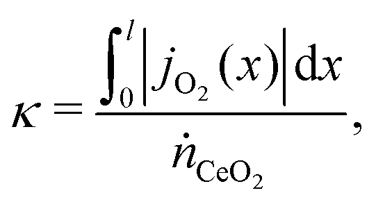
It is more convenient to formulated the problem to be independent of the exchanger size and the position coordinates. This is achieved here by defining an exchange coordinate κ, as the number of moles of species A that have been exchanged per mole of flow 1 entering the system, by a certain point x along the interface, which is given by
 | (2) |
With this change of coordinates eqn (1) becomes,
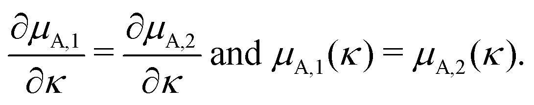
| μA,1(κ) ≥ μA,2(κ). ∀ κ ∈ [0, κtotal]. | (3) |
The conservation of mass can be applied to the exchange between the flows, meaning that the number of moles of A to have left flow 1, must be equal to the number of moles to have entered flow 2, at all points along the reactor interface. In a cocurrent system this statement is mathematically trivial and simply means that
| κ1 = κ2 ≡ κ, | (4) |
In a countercurrent system we have flow 2 reversed and so conservation of mass means that the exchange coordinate κ can be redefined in flow 2 by,
| κ1 = κ2 − κtotal ≡ κ, | (5) |
 | ||
| Fig. 3 A schematic showing the advantage of countercurrent flow over cocurrent flow, where the countercurrent case allows for a greater exchange of species. | ||
For the cocurrent case, the chemical potential μA,1 is expected to be a decreasing function of κ, and μA,2 an increasing function, which is illustrated in Fig. 3. This behaviour ensures thermodynamic stability, where any addition of species A to a solution should not decrease μA, and vice versa. Therefore, in a cocurrent system, it is sufficient to obey eqn (3) at the end point of the system κ = κtotal, and the thermodynamic upper bound for species exchange κtotal = κmax would be the case where they are equal at the outlet,
| μA,1(κtotal) = μA,2(κtotal). | (6) |
A countercurrent system is not so straightforward. Since flow 2's dependence on κ is reversed (eqn (5)), the chemical potentials μA,1 and μA,2 will both be decreasing functions of κ as illustrated in Fig. 3. This means that with non-linear dependence on κ, it may not be possible to have equal concentrations at ether of the end points, without violating eqn (3) somewhere in the domain κ ∈ (0, κtotal).
For smooth functions this implies that they could meet at one of the boundaries,
| μA,1(0) = μA,2(0) or μA,1(κtotal) = μA,2(κtotal), | (7) |
 | (8) |
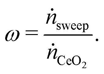
To determine the upper bound of species exchange for a given system one must first fix some parameters such as the temperatures and pressures of the streams. Another key physical parameter which can be set is the relative molar flow rates, which is denoted in this work by ω,
 | (9) |
| f1(T1,p1,μA,1,κ) = 0, | (10) |
| f2(T2,p2,μA,2,κ) = 0, | (11) |
A simple method of determining the thermodynamic limit on species exchange is then to start with κtotal = 0 and increase this value, until one of the limiting conditions are reached (6 for cocurrent systems, and 7 and 8 for countercurrent), or as is possible for countercurrent systems, all of the species is transferred.
If the flow's are in contact or separated by a thin membrane, most cases will have T1 = T2 and p1 = p2, but the methodology is by no means limited to these cases. For example one could conceivably have a pressure or temperature difference across a membrane, and as long as eqn (3) holds, then we can have spontaneous process with the transfer of species from flow 1 to flow 2. The temperature and pressure could also vary within the system. For example in an adiabatic reactor, where the temperature could also depend on the exchange coordinate T(κ) as a result of the heat of the reaction. The examples here are heat driven reactors, which are best approximated as isothermal rather than adiabatic, and so we set both temperatures and pressures to be equal and constant in both flows T1 = T2 = T and p1 = p2 = p.
It is important to also understand the context in which the model can be applied. Real countercurrent reactors are open systems which can have irreversible effects, such as diffusion along the flow's, and a more sophisticated model would be required to accurately predict performance. With the assumptions used here one can simply set an upper bound on species exchange. It therefore serves as a straightforward check of thermodynamic limits and a means of determining the potential for performance improvement over a cocurrent system. It should also be noted that changes in interface energy have been omitted from the analysis, which in some cases, such as bubble reactors, may play an important role.
Examples
This section illustrates the analysis of a number of countercurrent reactor systems and makes a brief comparison to previous models and experimental data available in the literature. The examples we consider are,• thermolysis of CO2 with oxygen removal across a membrane,
• dry reforming with oxygen exchange across a membrane,
• reverse water gas shift with oxygen exchange across a membrane,
• CeO2 reduction with a sweep gas removing oxygen,
which are illustrated in Fig. 4.
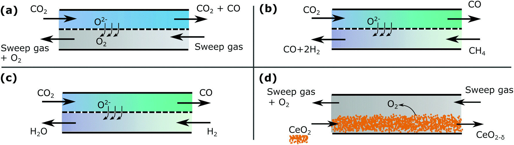 | ||
| Fig. 4 A schematic showing the examples (a–d) in countercurrent configuration. | ||
Cases (a) and (d) are solved analytically. Cases (b) and (c) are treated with a more robust numerical method utilizing the thermodynamic library Cantera,13 with a simple implementation of the methodology in python.†
(a) Membrane thermolysis
The idea of using a species selective membrane to separate the products of steam thermolysis has been proposed by Fletcher et al. as early as 1977,14,15 with the reaction given by,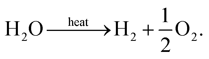 | (12) |
This direct thermolysis method has been experimentally demonstrated by Tou et al., using a concentrated solar powered reactor to split CO2 with an oxygen selective membrane made from ceria.12 In this system argon and carbon dioxide were arranged in countercurrent flow on either side of a ceria membrane, with the argon acting as an inert sweep gas to carry away oxygen produced by the thermolysis reaction,
 | (13) |
A schematic of the system can be seen in Fig. 4(a), which can be modeled according to the methodology described in the previous section to determine the thermodynamic limits. Note that the analysis presented would be identical if the CO2 were replaced with steam for H2O thermolysis.
The system is modeled as isothermal at a temperature of 1500 °C, and with both flows at a pressure of 1 bar, which allows for direct comparison of our model to the experimental work of Tou et al.12 Since oxygen is being exchanged between the two flows, we can define our exchange coordinate as
 | (14) |
The relative flow rate of the sweep gas to the CO2 is used as a free control parameter,
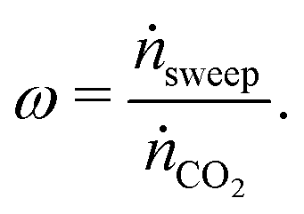 | (15) |
The thermodynamics of both flows can be well approximated as ideal gas solutions giving
 | (16) |
| pO2,1(κ) ≥ pO2,2(κ). ∀ κ ∈ [0, κtotal] | (17) |
For the sweep gas determining pO2(κ) is straightforward. Assuming we have a sweep gas with an oxygen impurity 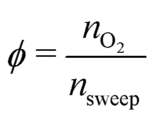 , flowing into the system, the partial pressure of oxygen in the sweep gas stream (flow 2) is given by
 | (18) |
 | (19) |
In the case of CO2, we must consider the equilibrium thermodynamics of the reaction given in eqn (13). The equilibrium composition of the CO2 splitting reaction is described by the variance in the Gibbs free energy,
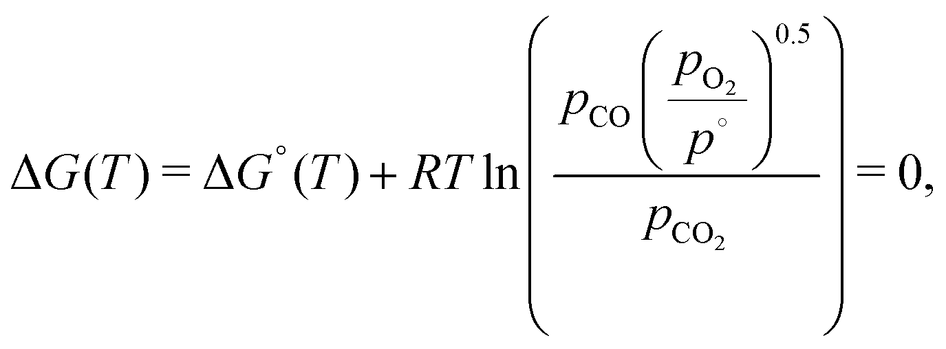 | (20) |
| pCO + pCO2 + pO2 = 1. | (21) |
 | (22) |
| pCO2(pO2) = p − pCO(pO2) − pO2, | (23) |
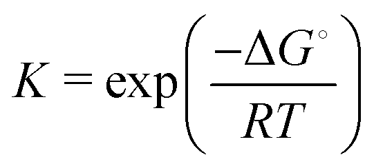 is the equilibrium constant.
The exchange coordinate in the CO2 flow can be formulated in terms of the partial pressures as,
 | (24) |
 | (25) |
 | (26) |
 .
.
The thermodynamic limiting case can then be found, by starting from κtotal = 0, and increasing this value until our stop conditions given in eqn (6)–(8) are reached, corresponding to κtotal = κmax. An example of the limiting case is illustrated in Fig. 5(a), for both cocurrent and countercurrent flow configurations. In the cocurrent case the sweep gas flow (CC) has an increasing dependence on κ and the partial pressures of the two flows meet at the maximum exchange extent, satisfying eqn (6). In the countercurrent case however both the CO2 flow and the sweep gas flow (CT) have a decreasing dependence on κ, and they share a common tangent satisfying the conditions given in eqn (8).
 | ||
| Fig. 5 (a) Plots of oxygen partial pressure vs. exchange extent κ for the CO2 stream given by eqn (25), cocurrent sweep gas flow CC given by eqn (18), and countercurrent sweep gas flow CT given by eqn (18) with κ′ = κmax − κ. The initial oxygen partial pressure in the sweep gas ϕp and the κmax in both cases are also labeled. (b) Mole fraction of CO in the CO2 stream plotted for cocurrent and countercurrent flow configurations at the same conditions listed in (a). Also shown is an experimental a point corresponding to Tou et al.'s experimental demonstration of this system in countercurrent configuration.12 | ||
Fig. 5(b) shows the dependence of the mole fraction of CO in the product stream, on the relative flow rate ω. This is equivalent to the CO2 conversion, where a value of one would indicate complete conversion. It can be seen that the countercurrent arrangement almost doubles the formation of CO (and κmax) relative to the cocurrent case for ω < 30. This is analogous to a countercurrent heat exchanger which can offer double the heat exchange of a cocurrent systems. In general, the conversion of CO2 to CO increases with increasing ω, and approaches a thermodynamic limit which is determined by the oxygen impurity in the sweep gas. The sweep gas impurity was selected to match conditions reported by Tou et al., where we have also included the conversion extent measured for their countercurrent reactor.12 The experimental value lies above the cocurrent model (CC), indicating that there was a real benefit to countercurrent operation. It also lies below the countercurrent thermodynamic limit, which it should.
Using the model applied by previous authors of matching the partial pressures at both the entrance and exit of the countercurrent reactor, means that the maximum exchange extent κmax only depends on the purity of the sweep gas.11,12 This is a counter intuitive result, where a fully pure sweep gas would then offer complete conversion. It can be seen by the differing shapes of the curves in Fig. 5(a), that matching both ends in the countercurrent case would not be possible, without violating the conservation of mass and/or the second law of thermodynamics (eqn (17)).
Correctly analysing the benefit of countercurrent operation for such a reactor shows that the conversion extent of CO2 (or H2O) at 1500 °C will be very small, unless huge quantities of very pure sweep gas are fed to the reactor. The thermodynamics of this membrane reactor system for thermolysis of CO2 or H2O, indicate that very high temperatures and/or very low oxygen partial pressures are required to achieve significant conversion of the reactants. This is unlikely to offer a practical or economically competitive means of converting heat to chemical energy.
(b) Membrane reforming
In the above section we used an analytical approach to solve a simple membrane countercurrent problem. In this case we look at a more complicated reaction system, and apply the methodology developed with a robust numerical analysis of the thermodynamic equilibrium. An interesting variation on the above process is to use methane instead of a sweep gas, where we then have methane partial oxidation taking place in flow 2, | (27) |
 | (28) |
For methane partial oxidation, there can also be the formation of CO2 and H2O, and so a simplified analytical approach will not suffice. Instead the thermodynamics of the reactions was modeled using the software Cantera,13 and it's gri30 database, which contains all of the relevant species. This software uses an element potential method to equilibrate an initially defined mixture of gases by minimizing the Gibbs free energy for the system.18
Since the same reaction is taking place in flow 1 as the previous example, our exchange parameter can again be defined by eqn (14), where we do not consider (or indeed expect) the reduction of CO to carbon, so that κ = 0.5 represents complete conversion. Here we consider the case with equal flow rates,
 | (29) |
 | (30) |
Similarly for the methane partial oxidation we consider an initial mixture of methane and find the thermodynamic equilibrium composition,
 | (31) |
 | ||
| Fig. 6 The numerical algorithm used to determine the maximum possible oxygen exchange in a dry reforming membrane reactor. This was implemented in Python using Cantera, and the code has been made publicly available.† | ||
Fig. 7(a) shows an example of the equilibrium partial pressure profiles with respect to the exchange coordinate κ. Here it can be seen that the CO2 oxygen release profile and CH4 oxygen uptake profile in countercurrent configuration allow for complete exchange (κmax,CT = 0.5) and complete CO2 conversion to CO, even at 600 °C. The cocurrent case on the other hand only exchanges about two thirds of the oxygen.
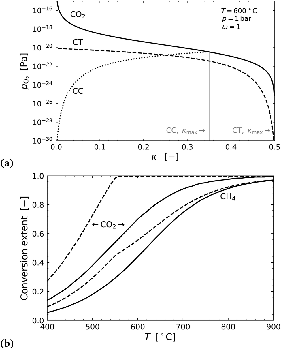 | ||
| Fig. 7 (a) Plots of oxygen partial pressure vs. exchange extent κ for the CO2 stream, the cocurrent CH4 flow CC, and countercurrent CH4 flow CT. (b) CO2 conversion (=2κ) and CH4 conversion, plotted as a function of the temperature for cocurrent with solid lines, and countercurrent with dashed lines. | ||
CO2 conversion alone is not enough to determine optimal operating conditions in this case. We must also consider CH4 conversion, as further oxidation of CO and H2 to CO2 and H2O in flow 2, can decrease the conversion of methane to syngas. The methane conversion can be determined from the mole fractions using the carbon balance,
 | (32) |
In the literature the results for conversion extents by Michalsky et al., fall well short of the thermodynamic limit,3 indicating that the system may have been kinetically limited. This is supported by the work of Jin et al., who used a catalyst in their membrane reactor and achieved higher conversions.16 The reactor of Jin et al. would be best modelled as cocurrent, where the authors used a ratio of 3CO2:1CH4, i.e. ω = 0.33. The conversion extent trends were similar to the thermodynamic analysis presented here, with a steeper dependence on temperature, which may indicate kinetic limitations at lower temperatures. Unfortunately, in these demonstrations the reactants are diluted in inert gases for experimental analysis purposes, which makes a more quantitative comparison difficult.
(c) Membrane reverse water gas shift
It is also interesting to consider other gases than CH4 to reduce CO2 in a membrane reactor. Of particular interest is to use a hydrogen flow giving flow 2 the oxidation reaction, | (33) |
 | (34) |
Taking renewable hydrogen followed by methanol synthesis as an example application, one could produce a suitable syngas by feeding three times as much hydrogen as CO2,
 | (35) |
:1 ensures that we will have a syngas composition suitable for methanol synthesis even without complete conversion of the CO2 according to the reactions,| 2H2 + CO → CH3OH, | (36) |
| 3H2 + CO2 → CH3OH + H2O. | (37) |
Since the same reaction is taking place in flow 1 as the previous two examples, our exchange parameter is again given by eqn (14). The thermodynamic library Cantera is used to model thermodynamics of each stream. The CO2 stream was modelled according to eqn (30), to determine the oxygen partial pressure pO2,1(κ). Similarly for the H2 stream the equilibrium is calculated according to,
 | (38) |
Fig. 8(a) shows an example of the partial pressure profiles with respect to the exchange coordinate κ. Here it can be seen that the CO2 oxygen release profile and H2 flow's oxygen uptake profile in countercurrent configuration allow for almost double the oxygen exchange as the cocurrent case. In the countercurrent case, more than 90% of the oxygen is exchanged corresponding to almost complete conversion of the CO2 to CO, even at just 500 °C.
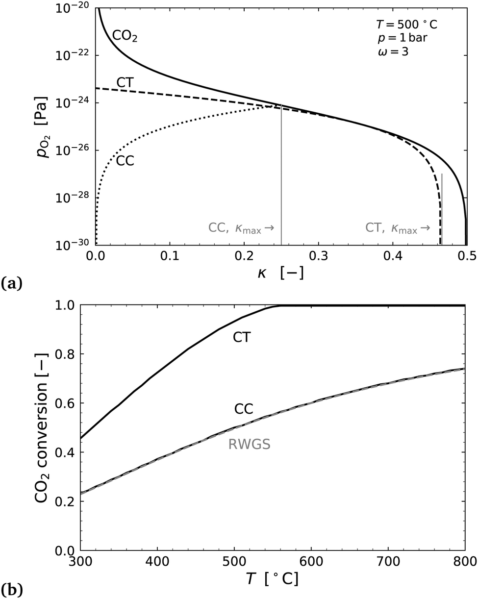 | ||
| Fig. 8 (a) Plots of oxygen partial pressure vs. exchange extent κ for the CO2 stream, the cocurrent H2 flow CC, and countercurrent H2 flow CT. (b) Maximum CO2 conversion (=2κmax) in flow 1 plotted as a function of the temperature for cocurrent and countercurrent flow configurations and for a simple co-feed reactor with 3H2:1CO (RWGS). | ||
The right hand side of Fig. 8 shows the conversion extent of CO2 for both cases, and for comparison an equilibrium calculation of the standard RWGS reaction with 3H2 + CO2. As one would intuitively expect the thermodynamic conversion limit in the cocurrent case is identical to that of the standard RWGS process.
The analysis shows that a countercurrent membrane reactor has promise for a low temperature reverse water gas shift process. The author could not find any experimental work or otherwise on this particular process idea, and it may be a novelty realised in this study. A physical implementation of this system have kinetic issues at low temperatures (<700 °C), and would likely require the use of catalysts on the membrane surfaces to realise the thermodynamic benefits illustrated in Fig. 8.
(d) Ceria reduction
Both H2O and CO2 can be split to produce fuel via a thermochemical redox cycle with ceria,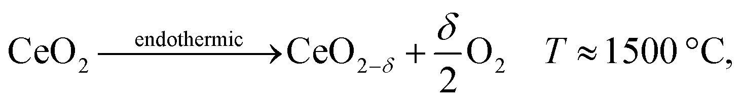 | (39) |
 | (40) |
Since the ceria is in the solid phase throughout the process, a flow of ceria particles through a reactor could be utilized, and a sweep gas could be arranged in countercurrent configuration as illustrated in Fig. 8. The oxidation step could also utilize a countercurrent reactor, but here we focus our analysis on the more critical endothermic reduction reaction.
Analysis of this system has proved to be controversial in the literature, with examples of modeling errors seen in the works of Davidson et al.7,8 They investigate this countercurrent reduction reactor with ceria, but apply the simplified assumption that partial pressures of oxygen at the exit of both streams will match the inlet of the other stream. This removes any need for a robust analysis, but predicts that oxygen partial pressures of 10−6 bar (or in principle, any pressure), can be achieved with no sweep gas at all or indeed any additional work. Despite this obviously paradoxical result, the model has been used by other authors,9,10 giving unrealistic expectations on the performance of countercurrent reactors for thermochemical redox cycles. Brendelberger et al. noticed that there was an error and published a more detailed analysis of this particular case, by assuming the partial pressure profiles share a common tangent at the ceria inlet.25 This is correct in some cases, but the profiles can also meet without a tangent at the ends, or indeed meet at any exchange extent κ. Li et al. also modeled this case, including the oxidation step of a thermochemical cycle, with a much more precise approach, combining conservation of mass with a Gibbs criterian dGT,p ≤ 0.4 They show very clearly that the partial pressures (or chemical potentials) in the limiting case can meet at any exchange extent, and clearly highlight the unphysical nature of previous models. The model was then utilized by these authors in a broader efficiency analysis of thermochemical fuel production.26
Although this particular case has already been solved, we apply the methodology formulated here, as an illustration of a system with reactions between two different phases in countercurrent flow, and indeed to compare the results to previous models.
Since oxygen is being exchanged between the two flows, we can define our exchange coordinate as
 | (41) |
| κ = 2δ, | (42) |
 | (43) |
The oxygen chemical potential, or oxygen activity of ceria can be converted to an equivalent oxygen partial pressure, so that we can determine pO2,1(κ). This is achieved using an analytical model developed by the author,27
 | (44) |
For the sweep gas pO2,2(κ) is given again by eqn (18), where the substitution κ′ = κmax − κ is used for the countercurrent case. This gives all the necessary formulae to use the methodology, according to the conditions given in eqn (6)–(8).
Fig. 9(a) shows an example of the limiting case, where the temperature T and oxygen impurity in the sweep gas ϕ, were selected to match the experimental demonstration of a countercurrent reactor performed by Scheffe et al.29 They experimentally demonstrated ceria reduction with a stream of falling particles (average size 12 μm) and a countercurrent sweep gas removing the oxygen, where I have used the data from Fig. 9 in their work for comparison. In Fig. 9(b), it can be seen that countercurrent operation offers an improvement in species transfer, relative to the cocurrent case, by a factor of approximately 1.5 for the conditions considered and for ω < 50. It can also be seen that the experimental values measured by Scheffe are greater than the thermodynamic limit for a cocurrent reactor, but less than he limit for a countercurrent reactor, and so support the model. The lower non-stoichiometry in the experiment could be due to the very short residents time for the particles in the hot zone of just one second, or partial re-oxidation of the material after exiting the hot zone. The thermodynamic model is also very idealised and does not consider diffusion of oxygen species along the direction of flow, which could also play an important role at such high temperatures. Nevertheless, it has served it's function well, which is to set an upper bound on the species transfer.
 | ||
| Fig. 9 (a) Plots of oxygen partial pressure vs. exchange extent κ for the flow of CeO2 particles, and the sweep gas in cocurrent flow CC, and countercurrent flow CT with κ′ = κmax − κ. (b) Maximum reduction extent δmax plotted against the relative flow rate ω, for the conditions listed in (a). Also indicated on the plot are the ω → ∞ limit, and the experimental results of Scheffe et al. for a countercurrent reactor. | ||
From the results it can also be seen that huge quantities of sweep gas are required in both cases to produce a very small non-stoichiometry in the ceria, which is well supported experimentally for both cocurrent and countercurrent reactors.21,29 This is in stark contrast to the results obtained using a simplified model.8 The model results do however, agree with the work of Li et al.4,25
Conclusions
The methodology presented should be very valuable in determining the limits of countercurrent reactor systems. Here we apply it to a number of cases in thermochemical fuel production, and the results indicate that countercurrent systems can offer higher potential for species transfer, typically on the order of 1–2 times greater than that of a cocurrent reactor in the cases analysed. This will depend on the specific reactions in the streams and values deviating from this general rule of thumb could be possible. Nevertheless this is a good first guess in most cases, and is analogous to the idea that a countercurrent heat exchanger can double the heat transfer relative to a cocurrent one. The results of the model are also supported by some experimental demonstrations of countercurrent reactors, where species exchange extents were greater than the cocurrent model, but less than our upper limit for countercurrent. Finally the analysis also highlights that an oxygen permeable membrane reactor has promising thermodynamics for low temperature reverse water gas shift using a countercurrent configuration.Conflicts of interest
There are no conflicts of interest to declare.Acknowledgements
Many thanks to Professor Aldo Steinfeld for his encouragement and support to pursue this manuscript as an independent research work, and to Maria Tou for many informative discussions on membrane reactors.References
- J. Piiper and D. Schumann, Respir. Physiol., 1967, 2, 135–148 CrossRef.
- Y. Shah, B. G. Kelkar, S. Godbole and W.-D. Deckwer, AIChE J., 1982, 28, 353–379 CrossRef CAS.
- R. Michalsky, D. Neuhaus and A. Steinfeld, Energy Technol., 2015, 3, 784–789 CrossRef CAS.
- S. Li, V. M. Wheeler, P. B. Kreider and W. Lipiński, Energy Fuels, 2018, 32, 10838–10847 CrossRef CAS.
- Y. Lee, Z. Wu and R. Torget, Bioresour. Technol., 2000, 71, 29–39 CrossRef CAS.
- D. R. Parisi and M. A. Laborde, Chem. Eng. J., 2004, 104, 35–43 CrossRef CAS.
- R. Bader, L. J. Venstrom, J. H. Davidson and W. Lipiński, Energy Fuels, 2013, 27, 5533–5544 CrossRef CAS.
- P. T. Krenzke and J. H. Davidson, Energy Fuels, 2015, 29, 1045–1054 CrossRef CAS.
- L. J. Venstrom, R. M. De Smith, R. Bala Chandran, D. B. Boman, P. T. Krenzke and J. H. Davidson, Energy Fuels, 2015, 29, 8168–8177 CrossRef CAS.
- B. D. Ehrhart, C. L. Muhich, I. Al-Shankiti and A. W. Weimer, Int. J. Hydrogen Energy, 2016, 41, 19904–19914 CrossRef CAS.
- L. Zhu, Y. Lu and S. Shen, Energy, 2016, 104, 53–63 CrossRef CAS.
- M. Tou, R. Michalsky and A. Steinfeld, Joule, 2017, 1, 146–154 CrossRef CAS PubMed.
- D. Goodwin, H. Moffat and R. Speth, Cantera: An Object-Oriented Software Toolkit for Chemical Kinetics, Thermodynamics, and Transport Processes, Version 2.3.0, 2017, DOI:10.5281/zenodo.170284.
- E. A. Fletcher and R. L. Moen, Science, 1977, 197, 1050–1056 CrossRef CAS PubMed.
- J. E. Noring, R. B. Diver and E. A. Fletcher, Energy, 1981, 6, 109–121 CrossRef CAS.
- W. Jin, C. Zhang, X. Chang, Y. Fan, W. Xing and N. Xu, Environ. Sci. Technol., 2008, 42, 3064–3068 CrossRef CAS PubMed.
- R. V. Franca, A. Thursfield and I. S. Metcalfe, J. Membr. Sci., 2012, 389, 173–181 CrossRef CAS.
- W. R. Smith, Theory and Algorithms, 1982 Search PubMed.
- B. Carvill, J. Hufton, M. Anand and S. Sircar, AIChE J., 1996, 42, 2765–2772 CrossRef CAS.
- B. Bulfin, J. Vieten, C. Agrafiotis, M. Roeb and C. Sattler, J. Mater. Chem. A, 2017, 5, 18951–18966 RSC.
- W. C. Chueh, C. Falter, M. Abbott, D. Scipio, P. Furler, S. M. Haile and A. Steinfeld, Science, 2010, 330, 1797–1801 CrossRef CAS PubMed.
- D. Marxer, P. Furler, M. Takacs and A. Steinfeld, Energy Environ. Sci., 2017, 10, 1142–1149 RSC.
- R. Panlener, R. Blumenthal and J. Garnier, J. Phys. Chem. Solids, 1975, 36, 1213–1222 CrossRef CAS.
- B. Bulfin, A. J. Lowe, K. A. Keogh, B. E. Murphy, O. Lubben, S. A. Krasnikov and I. V. Shvets, J. Phys. Chem. C, 2013, 117, 24129–24137 CrossRef CAS.
- S. Brendelberger, M. Roeb, M. Lange and C. Sattler, Sol. Energy, 2015, 122, 1011–1022 CrossRef CAS.
- S. Li, V. M. Wheeler, P. B. Kreider, R. Bader and W. Lipiński, Energy Fuels, 2018, 32, 10848–10863 CrossRef CAS.
- B. Bulfin, L. Hoffmann, L. de Oliveira, N. Knoblauch, F. Call, M. Roeb, C. Sattler and M. Schmuecker, Phys. Chem. Chem. Phys., 2016, 18, 23147–23154 RSC.
- M. Takacs, J. Scheffe and A. Steinfeld, Phys. Chem. Chem. Phys., 2015, 17, 7813–7822 RSC.
- J. R. Scheffe, M. Welte and A. Steinfeld, Ind. Eng. Chem. Res., 2014, 53, 2175–2182 CrossRef CAS.
- S. Li, P. B. Kreider, V. M. Wheeler and W. Lipiński, J. Sol. Energy Eng., 2019, 141, 021012 CrossRef.
Footnote |
| † https://github.com/bulfinb/countercurrent_reactor_algorithm. |
| This journal is © the Owner Societies 2019 |