Nonadiabatic dynamics simulations of singlet fission in 2,5-bis(fluorene-9-ylidene)-2,5-dihydrothiophene crystals

Abstract

We present simulations of the singlet fission dynamics in 2,5-bis(fluorene-9-ylidene)-2,5-dihydrothiophene (ThBF), a thienoquinoid compound recently investigated experimentally by Kawata et al. The simulation model consisted of two ThBF molecules embedded in their crystal environment. The aim was to understand the singlet fission mechanism, and to predict the excited state lifetimes and the singlet fission quantum yield, hitherto unknown. The simulations were performed by the trajectory surface hopping approach with on-the-fly calculations of the electronic wave functions and energies by the semiempirical FOMO-CI method. We found that the initially photogenerated excitonic bright state decays to the lower dark state with a biexponential behaviour, essentially due to transitions to other close lying states. The dark state in turn decays with a lifetime of about 1 ps to the double triplet ¹TT state, which is long-lived, as ascertained by performing a simulation with inclusion of the spin–orbit coupling. The singlet fission quantum yield is predicted to be close to the theoretical maximum of 200%. In view of using this thienoquinoid compound in photovoltaic devices, a major drawback is the low energy of the T₁ state at its equilibrium geometry.

---

1 Introduction

Singlet fission (SF)^2–4 is a spin-allowed radiationless process which occurs in a ps or sub-ps time scale, whereby a photogenerated excited singlet state in (at least) two interacting chromophores A and B converts into a pair of localised T₁ triplet states that are coupled into an overall singlet, indicated as ¹TT. The initially excited singlet can be localised on one chromophore, S₁(A) + S₀(B) or S₀(A) + S₁(B), or be instead the result of exciton coupling between the two chromophores in their S₁ states.⁵ SF has recently attracted much attention due to its potential to allow overcoming the theoretical Shockley–Queisser limit for the power conversion efficiency of a single junction solar cell, which is about 32%.⁶ In order to get a large singlet fission quantum yield, the transition from the initially excited state to ¹TT has to be faster than other intra- and inter-molecular processes, such as internal conversion (IC) and intersystem crossing (ISC). Considering the excitation energies of two identical chromophores, it is then required that ΔE(S₁) ≥ 2ΔE(T₁), so that SF is exoergic. Additionally, the ¹TT state should not be depopulated by internal conversion to the ground state nor by ISC to a triplet state T_n(A) + S₀(B) or S₀(A) + T_n(B). To this aim, no triplet should lie close or below the ¹TT state: ΔE(T₂) > 2ΔE(T₁). Actually, it is desirable that ΔE(T₂) > ΔE(S₁), to avoid fast ISC from the initially excited state. Finally, molecules that are going to be used as SF chromophores in photovoltaic cells must also satisfy other properties, such as broad and intense absorption, T₁ energy larger than the semiconductor band gap, and chemical stability under solar irradiation.⁷

Two main classes of chromophores have been found to meet the energetic requirements for SF: alternant hydrocarbons, especially polyacenes, and biradicaloids.^2–4 Recently, non-polycyclic aromatic molecules based on the thienoquinoidal structure have been synthesised. Their ability to undergo SF has been proven by using them, in crystalline form, as the electron donor in organic photovoltaic devices and by detecting the magnetic field dependence of the photocurrent.¹ Moreover, in the same work the energies of the excited singlet and triplet states were determined by absorption spectroscopy and by DFT/TD-DFT calculations. The basic energetic condition ΔE(S₁) ≥ 2ΔE(T₁) was found to be fulfilled. However, the SF mechanism, its time scale and the possible competing processes are hitherto unknown. The present work sheds light on the photodynamics of the simplest of such molecules, namely 2,5-bis(fluorene-9-ylidene)-2,5-dihydrothiophene (ThBF, see Fig. 1), by means of trajectory surface hopping simulations.^8–11

Fig. 1 Chemical structure of ThBF.

Time-resolved spectroscopy techniques such as transient absorption, up-converted fluorescence, time-resolved two-photon photoemission, and 2-D electronic spectroscopy have been applied to other chromophores in order to investigate the dynamics of SF, reveal its time scales and some important parameters that determine its efficiency.^12–17 The theoretical modelling of SF dynamics often complements the experimental findings and allows the SF mechanism to be explored, which may not be univocally inferred from the experimental results. In the present case the computational simulation comes first and can be a useful basis to plan transient spectroscopy experiments.

Both fully quantum mechanical (QM) and mixed quantum-classical theoretical methods have been applied to the study of SF. Important insight was gained by Berkelbach et al. by applying Redfield theory to fully QM model systems with electron–phonon coupling.^18–20 Their results suggest the importance of charge transfer states in the SF dynamics of pentacene. Tamura et al. employed the multiconfigurational time-dependent Hartree QM approach to investigate the SF mechanism in a pentacene derivative and in rubrene.²¹ They showed how the crystal structure of the pentacene derivative favours a coherent and ultrafast population transfer to the ¹TT state, while in rubrene thermally activated symmetry-breaking vibrations are needed in order to guarantee a non-vanishing coupling between the initial and final states. Mixed quantum-classical methods, such as nuclear trajectories with surface hopping (SH),¹¹ have the advantage of allowing to explore the full nuclear phase space and to extend the integration time to several picoseconds. In particular, while small amplitude internal motions can be efficiently treated by fully quantum models with harmonic potentials,^18–20 it would be more difficult to set up such models for the relative motions of monomers in a molecular crystal (see discussion about the geometry changes that bring about transitions to the ¹TT state in Section 4). SH simulations were already performed to study SF in polyacenes.^22,23 In this work, we applied the SH model by computing on the fly the electronic energies and wavefunctions of the pair of molecules undergoing photodynamics, by means of the semiempirical floating occupation molecular orbital configuration interaction (FOMO-CI) method.^8,11 The crystal environment was described by molecular mechanics (MM) and its effect was taken into account by the QM/MM variant of the FOMO-CI method.⁹ All the semiempirical calculations and the QM/MM simulations in this work were performed using a modified version of MOPAC2002,²⁴ interfaced with the TINKER molecular mechanics package²⁵ version 6.3, when appropriate.

Section 2 compares the DFT and semiempirical results for the ThBF monomer, Section 3 introduces the QM/MM description of a ThBF dimer embedded in the crystal structure and Section 4 describes the excited state dynamics.

2 Monomer calculations and semiempirical method

In order to characterise the excited states of the ThBF molecule, we performed DFT and TD-DFT calculations with the B3LYP functional and the 6-31G+(d) basis set. TD-DFT was used to calculate the vertical excitation energies (ΔE_vert) of both states, and also to optimise the geometry of S₁. For the T₁ optimisation we used DFT rather than TD-DFT, because the closeness of the T₁ and S₀ energies makes the latter method not reliable at such geometries. The results, presented in Tables 1 and 2, show that ThBF is mainly a closed shell molecule with an extended conjugated π system, the core of which is made of three π bonds, one belonging to the dihydrothiophene moiety and two connecting it to the fluorene groups. This view is supported by the bond lengths reported in Table 1 and by the nature of the occupied orbitals (see Fig. S1 in the ESI†).

Table 1 Geometrical parameters of the ThBF monomer (bond lengths in Å and dihedral angles in degrees)

State	Method	R(C12C14)	R(C14C15)	R(C15C16)	∠C13C12C14C15
a Molecular crystal.
S0^a	X-ray diffraction^1	1.38	1.43	1.33	2.1
S0	DFT B3LYP/6-31G+(d)	1.38	1.44	1.36	10.4
S1	TD-DFT B3LYP/6-31G+(d)	1.43	1.41	1.40	23.5
T1	DFT B3LYP/6-31G+(d)	1.44	1.39	1.41	33.7
S0	FOMO-CI, PM3	1.35	1.46	1.35	2.2
S0	FOMO-CI, reparam. PM3	1.38	1.48	1.37	1.1
S1	FOMO-CI, reparam. PM3	1.38	1.48	1.37	0.1
T1	FOMO-CI, reparam. PM3	1.44	1.44	1.40	16.7

---

Table 2 Transition energies (eV) of the ThBF monomer

Method	ΔEvert(S1)	ΔEadia(S1)	ΔEvert(T1)	ΔEadia(T1)
a The ONIOM procedure was applied to simulate the effect of crystal embedding.^1
Absorption spectrum^1	2.30	∼2.2
TD-DFT B3LYP/6-311G+(d)^a	2.22
ΔSCF B3LYP/6-311G+(d)^a			0.90
TD-DFT B3LYP/6-31G+(d)	2.31	2.09	0.97
ΔSCF B3LYP/6-31G+(d)			1.20	0.77
FOMO-CI, PM3	2.96	2.86	1.84	1.08
FOMO-CI, reparam. PM3	2.17	2.16	0.91	0.54

---

The excitations that characterise the T₁ and S₁ states mainly concern this triene system, in which the HOMO and LUMO π orbitals are well localised (Fig. S1, ESI†). Looking at the nodal character of the LUMO, it is clear why the bond length alternation is reversed in going from the ground state to the excited ones. Actually this feature is much more pronounced in T₁ than in S₁, so the bonds linking the dihydrothiophene and fluorene moieties have an increasing single bond character in the order S₀ < S₁ < T₁. Therefore, the twisting of these bonds (dihedral angles C₁₃C₁₂C₁₄C₁₅ and C₁₆C₁₇C₁₈C₃₀), driven by the repulsion of the pairs of H atoms bound to C₁/C₁₅ and C₁₆/C₂₉, also increases in the same order. Consistently with the larger geometrical change from the Franck–Condon point to the excited PES minimum, the difference between ΔE_vert and the adiabatic transition energy ΔE_adia is much larger in T₁ than in S₁.

To choose the semiempirical Hamiltonian and other details of the FOMO-CI calculations, we compared the FOMO-CI description of the S₀, S₁ and T₁ states of ThBF with the experimental and DFT/TD-DFT results, focussing on the ΔE_vert and ΔE_adia transition energies. We tried the MNDO, AM1, PM3 and PM5 Hamiltonians with three different CAS-CI active spaces, i.e. CAS(6,5), CAS(6,4) and CAS(2,2). Moreover, we also varied the Gaussian width w which determines the floating occupation numbers (w = 0.1, 0.15, and 0.2 a.u.).⁸ In all cases the description of the electronic structure was qualitatively correct, but the transition energies turned out too large (see for instance the PM3 entry in Table 2). Therefore, we proceeded to optimise the semiempirical parameters for the most promising combinations of the semiempirical Hamiltonian, Gaussian width and active space, using a well tested procedure.^26,27 The best results were obtained with the PM3 Hamiltonian, the active space CAS(2,2) and the Gaussian width w = 0.1 a.u. The excitation energies are well reproduced, within the uncertainty of the available data. The torsion angles are underestimated, as can be seen in Table 1, and only the T₁ state presents a non negligible twisting. However, this feature seems to be scarcely important in the simulations we performed, because in the crystal structure all molecules are practically planar, due to the strong stacking interactions.

3 Ground state crystal structure and dynamics

We optimised the crystal structure of ThBF by using the OPLSAA force field,²⁸ starting from the X-ray data of Kawata et al.¹ The atomic charge parameters were obtained from a DFT calculation employing the B3LYP functional and the 6-311+G(d,p) basis set, by fitting the electrostatic potentials using the CHELPG scheme with the additional constraint to reproduce the overall molecular dipole moment.²⁹ The crystal structure contains four molecules per unit cell, which belong to four equivalent slipped stacks with orientations only differing in the slope of the molecular planes and/or by a rotation of 180° (see Fig. 2 and 3).

Fig. 2 Unit cell of the ThBF crystal, as obtained by optimisation with the OPLSAA force-field.

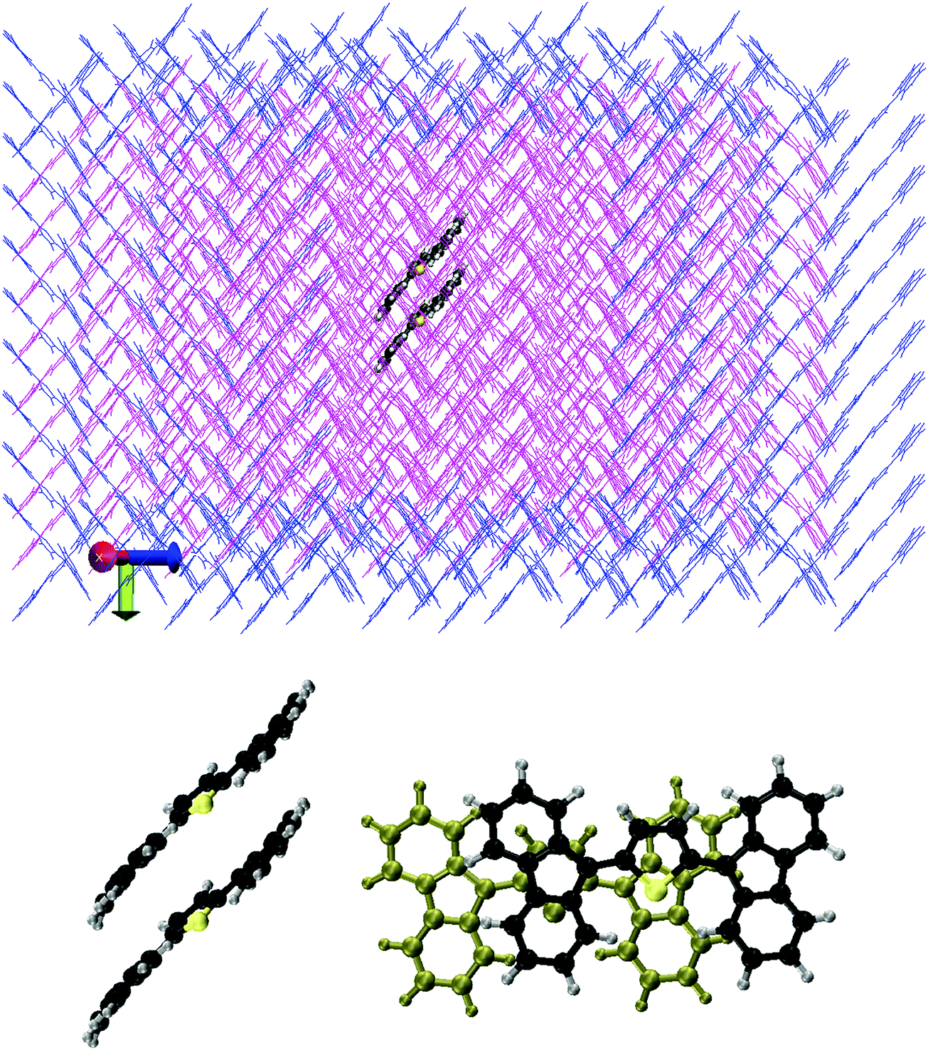Fig. 3 Upper panel: the representation of the QM and MM subsystems of the ThBF crystal structure. The space-filling model represents a pair of molecules in the QM subsystem (C atoms are in black, S atom in yellow, and H atoms are in grey), while the line model in magenta and blue represents molecules in the MM subsystems which move freely and are kept frozen, respectively, during the dynamics simulations. Lower panel: the mutual position and orientation of the two QM molecules in a slip-stack arrangement, shown from two different points of view (in the right hand side, the farther molecule is depicted in a different color for a better clarity).

The optimised crystal structure was then taken as the starting point for a MD simulation employing the NVT ensemble with a constant temperature of 300 K for 10 ns. Periodic boundary conditions were imposed during this thermal equilibration. The last frame of the periodic MD simulation was then used to start a QM/MM thermal trajectory for a cluster containing 490 molecules, arranged in a 7 × 7 array of 49 slipped stacks of 10 molecules each (see Fig. 3). Two molecules, the fifth and sixth in the central stack, were represented at the QM level and the others at the MM level. 162 MM molecules at the boundary of the cluster were kept frozen in order to keep the rigidity of the crystal structure, while 326 MM molecules plus 2 QM molecules were freely moving during the dynamics. In the slip-stack arrangement the molecules are approximately planar, with their planes 3.6 Å far apart and a slip of 3.5 Å, such that a fluorene group of one molecule overlaps with the dihydrothiophene group of the other molecule. This is in particular the relationship between the two QM molecules, as represented in Fig. 3. The QM molecules were treated by the FOMO-CI method as described in the previous section, using an active space CAS(4,4) which is equivalent to the CAS(2,2) we selected for the monomer. The MM molecules were treated using the OPLSAA force field as mentioned above and electrostatic embedding was applied to represent the interactions between the QM and MM subsystems.⁹

The QM/MM ground state equilibration was performed by employing the Bussi–Parrinello thermostat³⁰ for 14 ps with a time step of 0.1 fs and a constant temperature of 300 K. To monitor the progress of the equilibration, we computed the total energy of the cluster (see Fig. S2, ESI†) and the transition energies from the ground state to the eight lowest excited singlet states of the two QM molecules (see Fig. 4). In discussing the excited singlet states of the molecular pair we shall adopt the notation S[n], indicating the n-th adiabatic singlet state in energy ordering, in order to distinguish them from the single molecule ones (S₀, T₁, S₁, etc.).

Fig. 4 Excitation energies of eight singlet states obtained during the QM/MM ground state equilibration as a function of time.

As can be deduced from the monomer excitation energies, the S[1] state, with an average excitation energy of 1.7 eV, most of the time is essentially the ¹TT state. S[2] and S[3] are mainly linear combinations of the S₁ states localised on each of the two QM molecules, S₁(A)S₀(B) and S₀(A)S₁(B). Since the two molecules are oriented essentially in the same way, the lower state, S[2], is the dark combination, and the higher one, S[3], is bright.⁵ The average of their energies is about 2.1 eV, with an exciton splitting of 0.25 eV. S[4] and the higher singlets are mainly of charge transfer (CT) nature. The energy profiles of Fig. 4 confirm that the basic energetic condition for SF is satisfied, in the sense that the process is slightly exoergic even starting from the lower excitonic state, i.e. the dark state S[2]. However, we note that the S[2] and S[3] transition energies undergo very small oscillations, with an amplitude of the order of 0.05 eV, whereas the energy of other states is much more sensitive to the small geometry changes occurring during the thermal trajectory. In particular, the S[1] transition energy fluctuates by about ±0.5 eV. This is consistent with the difference between ΔE_vert and ΔE_adia found in the T₁ state of the monomer, much larger than in S₁, meaning that the ¹TT PES in the Franck–Condon region is quite steep (see Table 2). In fact, one can see that from time to time the energy fluctuations bring S[1] at the same level where normally one finds S[2], or, more seldom, even S[3]. This is a hint that the ¹TT and the exciton states can switch in energy, a fact that must be kept in mind when discussing the excited state dynamics simulations.

We also computed the S[0] → S[n] transition dipole moments, from which we obtained the absorption spectrum in the form of an energy histogram, by averaging over the whole QM/MM thermal trajectory (see Fig. 5). The maximum of the main band is at 2.28 eV, in good agreement with the experimental spectrum,¹ and the oscillator strength per molecule is f ≃ 1.0 (f = 1.17 for the vertical excitation of the monomer at the TD-DFT/B3LYP level). The band is however too narrow and tall, due to the common problem of neglecting the zero point vibrations in classical simulations, but probably also to a somewhat underestimated slope of the excited state PES around the Franck–Condon point by the FOMO-CI calculations. In fact, the dominant contribution is due to the bright state, i.e. S[3], which shares with the S₁ state of the monomer the small difference between the ground and excited state equilibrium geometries. A small contribution to the main band is also due to S[4]. The S[1] and S[2] states show very weak absorptions between 1.95 and 2.10 eV: since the transition to ¹TT is forbidden unless some mixing with other states occurs,³¹ the real responsible for this weak band is the dark state, which is most of the time S[2] and more seldom S[1]. For a similar reason, S[2] also contributes very weakly to the main band: this occurs when ¹TT is temporarily higher in energy than both exciton states and S[2] is then the bright state. These observations confirm the switching of states already discussed with regard to Fig. 4.

Fig. 5 The computed electronic absorption spectrum obtained as the average from 0 to 14 ps of the QM/MM ground state equilibration.

4 Excited state dynamics simulations

The time dependence of the total energy (Fig. S2, ESI†), of the excitation energies (Fig. 4) and of the absorption spectrum (Fig. S3, ESI†) shows that after 2 ps the QM/MM cluster is sufficiently equilibrated, i.e. the perturbation due to the small difference between the full MM and the QM/MM treatments has died off. Therefore, the sampling of the initial conditions for the excited state trajectories was done by taking at random a set of phase points belonging to the QM/MM ground state equilibration trajectory, with the exclusion of the first 2 ps. For each phase point, a number of trajectories (0, 1 or more) were launched by vertical transitions to the excited states lying within 1.6 to 2.8 eV from the ground state energy. The probability of starting a trajectory in state S[n] is taken proportional to the squared S[0] → S[n] transition dipole moment.¹¹ As a result, 484 trajectories were launched, of which 6 started in S[2], 443 in S[3], 34 in S[4] and 1 in S[5], consistent with the dominant role of S[3] (the bright state) in the absorption band.

The excited state dynamics was modelled by surface hopping^8,11 with overlap based decoherence corrections.¹⁰ A time step of 0.2 fs was used to integrate the classical trajectories up to the final time of 2.5 ps. The parameters for the decoherence corrections were σ = 1.0 a.u. (Gaussian width) and S_min = 0.005 (minimum overlap). The integration of the time-dependent Schrödinger equation for the electrons was performed by an algorithm that guarantees stable results even in the case of very weak interactions, i.e. of narrowly avoided crossings.^8,32

The state populations as functions of time are presented in Fig. 6. The population P_n is computed as the fraction of trajectories running on the adiabatic PES number n, i.e. those trajectories for which S[n] is the “current state” (n = 0…8). Table 3 shows the average transition rates between pairs of states, i.e. the number of hops per picosecond, divided by the number of trajectories, along the whole simulation. The states S[4] to S[8] are grouped together, because most of their population is concentrated in S[4] and because of the fast transition rates between them (see the more detailed account of hopping rates provided in Table S1, ESI†). It should be kept in mind that many hops are due to energy switches between two states, for instance the bright state and the mixed charge transfer state that are usually S[3] and S[4]. In most cases, due to the weak interactions between the two states, the system goes diabatically through the avoided crossing, i.e. a transition between the adiabatic states occurs by leaving the nature of the electronic state unchanged. Since the energy changes that cause such switches usually last for a short span of time (see Fig. 4), we have some very large m → n and n → m rates with smaller net rates. This is the case for the S[4] → S[3], S[3] → S[2] and S[2] → S[1] transitions.

Fig. 6 Adiabatic state populations (upper panel) and the fitting obtained by a simple rate model.

Table 3 Hopping rates (ps⁻¹)

State	State	Rate^a	Rate^a	Net rate^b
m	n	m → n	n → m
a Average rate over the whole simulation in 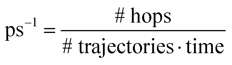. b Net rate = difference between the m → n and the n → m rates.
S[1]	S[0]	0.000	0.001	−0.001
S[2]	S[0]	0.042	0.018	0.024
S[3]	S[0]	0.007	0.007	0.000
S[4–8]	S[0]	0.010	0.017	−0.007
S[2]	S[1]	3.540	3.192	0.349
S[3]	S[1]	0.016	0.031	−0.015
S[4–8]	S[1]	0.002	0.031	−0.028
S[3]	S[2]	3.326	2.165	1.160
S[4–8]	S[2]	1.030	1.759	−0.729
S[4–8]	S[3]	5.303	4.520	0.783

---

The bright state S[3], which is initially the most populated, decays rapidly within 100–200 fs, transferring population to S[4], which is very close in energy, and to a lesser extent to the higher states S[5]–S[8], as well as to the lower lying S[2], i.e. the dark state. The upper group of states (S[4] and the higher ones) keep exchanging population with S[3], so in the long run they decay approximately at the same rate. Moreover, these states acquire population from S[2] and transfer it to S[3], so they effectively slow down the S[3] → S[2] decay. Of course this effect is negligible at the beginning of the simulation, when the population of S[2] is very low, and becomes important after ≈200 fs: as a result, the decay of S[3] and of the upper states is initially very fast, but gets slower after a few hundred fs. S[2] in turn decays to S[1], the ¹TT state, and also, quite marginally, to S[0]. The decay of S[2] is slower than that of S[3], so its population accumulates, reaches a maximum around 500 fs and then decreases smoothly.

Since we are dealing with adiabatic states that are linear combinations of the diabatic ones (S₀(A)S₀(B), S₁(A)S₀(B), S₀(A)S₁(B), ¹TT and the CT states), our simulations do not provide direct evidence of the importance of the electronic couplings in the diabatic representation. Therefore, we resorted to a diabatisation procedure based on orbital localisation, devised ad hoc for the FOMO-CI method.³³ In Table S2 (ESI†), we report the electronic hamiltonian matrix computed in the diabatic basis for an arrangement of two ThBF molecules in their planar S₀ equilibrium geometry with an overall C₂ symmetry. We see that the direct couplings and are extremely small, whereas much larger matrix elements couple both ¹TT and the localised singlet states with the CT states. The interaction mediated by the CT states^3,33 can be evaluated to about 0.9 meV and is therefore the main cause of transitions from the localised singlets (or rather their combination, the dark state) to the ¹TT state. However, because of the different energy gaps, S[4] and higher states, which are essentially of CT nature, are easily populated starting from S[2] and S[3], but do not exchange population with S[1], i.e. the ¹TT state.

The adiabatic energy difference at the S[2] → S[1] hopping events is small, 0.027 eV in the average, because of the weak interaction between the dark and the ¹TT states. Note that surface hopping performs very well in the presence of weakly avoided crossings or conical intersections with small couplings, whereby the transition events are well localised in time and space,^34,35 so quantum effects are unlikely to be important in this case. The quasi-degeneracy between S[1] and S[2] is reached thanks to a substantial energy lowering of the upper state in going from the initial geometry (Franck–Condon region) to the hopping ones. Taking as reference the ground state S[0], the lowering of S[1] is about −0.6 eV (see Table S3, ESI†). As already mentioned, in the ThBF monomer the difference ΔE_adia − ΔE_vert for the first excited singlet is quite small, so the geometrical changes that cause such energy lowering must involve the relative position and orientation of the two monomers. In fact, Table S3 (ESI†) shows almost no change in the four internal coordinates already chosen to characterise the equilibrium geometries of the monomer states (Table 1), while the distances between atoms of monomer A and the corresponding atoms of monomer B decrease noticeably in going from the Franck–Condon region to the hopping geometries. More in detail, the distance between the two dihydrothiophene cores decreases by 0.16 Å (averaging over the five heavy atoms), two of the fluorene groups get closer by about 0.2 Å, while the other two do not move appreciably. The energetic effects are due in part to the increase of the excitonic coupling, as shown by the S[3]–S[2] (dark to bright state) energy splitting, which averages to 0.28 eV at the initial geometries and to 0.54 eV at the hopping ones. An important contribution must also come from the change in the monomer-to-monomer interaction energy, which is affected by the difference in the charge distribution caused by excitation. In fact, the electronic density of the LUMO is more spread than that of the HOMO, and shifted away from the S atom, so that the S₁ state of the monomer develops a large dipole moment (3.7 debye at the FOMO-CI level, to be compared with 0.3 debye of the ground state).

In order to extract the state lifetimes from the simulation data, the populations were fitted by a simple consecutive decay model:

S[3], S[4]…S[8] → S[2] → S[1], S[0] (1)

Since the decay of S[3] and higher states follows two different regimes in the short and long time range, we modelled the sum of their populations with a biexponential function:

P_3–8(t) = P_3–8(0) [We^−t/τ₃ + (1 − W)e^{−t/τ₃′}] (2)

By assuming a fixed decay rate 1/τ₂ for S[2], its population is then

P₂(t) = Xe^−t/τ₃ + X′e^{−t/τ₃′} + Ye^−t/τ₂ (3)

whereOf course, the sum of the populations of the two lowest states is

P₀(t) + P₁(t) = 1 − P_3–8(t) − P₂(t) (5)

The initial populations P_3–8(0) = 0.988 and P₂(0) = 0.012 being known, the parameters τ₃, τ₃′ and W were determined by fitting P_3–8(t), and τ₂ by subsequently fitting P₂(t). This procedure yielded τ₃ = 0.11 ps, τ₃′ = 1.05 ps, τ₂ = 1.32 ps and W = 0.645. Time-resolved spectroscopy experiments should be able to confirm these data.

One of the main goals of this work was to determine the quantum yield of singlet fission, which is apparently very high since the S[1] state is by far the most populated at the end of the simulation. However, as already observed, one cannot take for granted that S[1] is univocally identified with the ¹TT state. Therefore, we extracted the ¹TT population from the simulation data in a different manner. We first identify the ¹TT state among the nine adiabatic singlets considered in the simulation, as the one that is closest to be a double excitation. In practice, given the four diagonal elements ρ_n,ii of the density matrix of state n restricted to the active space, we compute the index

and we identify the ¹TT state as the state S[n] with the smallest value of V_n. Then, we evaluate the ¹TT population by computing the fraction of trajectories F_¹TT in which n is the current state. Fig. S5 (ESI†) shows that F_¹TT and P₁ practically coincide, especially towards the end of the simulation. In fact, once the system settles in the deep minimum of the S[1] PES and the vibrational energy excess of the excited molecules starts to be dissipated by coupling with other modes, the probability that the ¹TT state and the dark state switch in energy fades away. So, the singlet fission quantum yield can be evaluated as twice the asymptotic S[1] population (two triplet states for every dimer that reaches the S[1] state). We can assume that in the S[2] decay, the branching ratio between S[0] and S[1] is the ratio of their final populations at t = 2.5 ps: P₀/P₁ = 0.022. So, the computed singlet fission quantum yield is 1.96, close to the theoretical maximum.

This high quantum yield seems to contrast with the low power conversion efficiencies measured in photodevices using ThBF (at best, about 1%), but other factors may explain such failure.¹ A feature highlighted in this work, namely the low adiabatic transition energy of the T₁ state of ThBF (see Table 2), is probably an important drawback. The value of ΔE_adia(T₁) sets an upper limit to the energy available to produce a charge separation: 0.77 eV according to ΔSCF DFT, or 0.54 eV according to FOMO-CI. However, the process is more probably “vertical”, i.e. it takes place at a fixed geometry corresponding to the minimum of the T₁ PES. Then, the energy difference with respect to the ground state further reduces to 0.27 eV, according to FOMO-CI. We conclude that, within this class of compounds, it is probably worth trying molecules with higher T₁ and S₁ energies.

A limitation of our model, namely the fact that only two molecules are treated at the QM level, in principle might lead to overestimate the singlet fission quantum yield. In fact, taking into account the delocalisation over more than two monomers, the lowest excitonic state would be lower in energy than the dimer dark state. If such a state be lower or of comparable energy with the ¹TT state, the quantum yield might considerably decrease. However, as already discussed when comparing the ¹TT state and the S[1] populations, at long times the system settles in the minima of the PESs and the ¹TT minimum is sufficiently low as to exclude an energy switch even with very delocalised excitonic states. In fact, according to the ΔE_adia values of Table 2, the ¹TT equilibrium energy is 1.1–1.5 eV. Concerning the lowest excitonic state, the theoretical limit for the energy lowering with respect to the monomer of a very delocalised state is twice the lowering observed in the dimer, i.e. about 0.25 eV, which places such a state at 1.9–2.0 eV, well above ¹TT (here we assume delocalisation over many monomers along a single stack and we take into account first-neighbour interactions only). Of course, delocalisation over more than two monomers can also change the couplings and therefore the transition rates. Simulations of the same type here described, but with three QM molecules instead of two, are being performed in order to investigate delocalisation effects.

The small energy gap between T₁ and S₀ at the T₁ equilibrium geometry has potentially another negative consequence. In fact, the same energy gap separates the ¹TT state from the two lowest triplet states in the dimer. Such triplets are almost degenerate, being essentially two equivalent excitations localised on each monomer, T₁(A)S₀(B) and S₀(A)T₁(B), or linear combinations thereof. Their energy proximity to the ¹TT state may facilitate the intersystem crossing (ISC) ¹TT → T[1] or ¹TT → T[2], so shortening the lifetime of ¹TT. To investigate this possibility, we performed a simulation taking into account the spin–orbit coupling (SOC), hereafter indicated as the “SOC simulation”, to distinguish it from the “singlet-only simulation” discussed till now. It included, in addition to the five most important singlet states (S[0] to S[4]), also five triplet states and one quintet state. The third triplet, T[3], and the quintet, Q[1], are the higher spin combinations of the double triplet excitation, almost degenerate with the ¹TT state. The sampling of initial conditions was more limited than in the singlet-only simulation, resulting in 66 trajectories. The SOC was treated in a semiempirical manner as described in previous work.^27,36 One parameter ξ for each heavy atom enters the one electron effective spin–orbit Hamiltonian adopted in our calculations.³⁶ For the carbon atoms we chose ξ_C = 28.6 cm⁻¹, that fits the splitting of the ³P ground state of the C atom. Actually the value of ξ_C turned out to be almost irrelevant in determining the SOC between the states of ThBF we are interested in, the largest contribution being due to the S atom. To fix the ξ_S value for sulphur, we determined the SOCs between the first three electronic states at the CASSCF(6,6) level with the ANO basis set³⁷ contracted to S,C[3s2p1d]/H[2s1p], at the DFT equilibrium geometry of S₀. The SOC between S₀ and T₁, expressed as norm of the coupling vector for the three triplet components, was 2.7 cm⁻¹, and between S₁ and T₁, 0.9 cm⁻¹. These rather small values are due to the scarce involvement of the S atom in the HOMO and LUMO orbitals. At the FOMO-CI level, using ξ_S = 275 cm⁻¹, we get 2.8 cm⁻¹ for the S₀–T₁ SOC, and zero for the S₁–T₁ SOC. The latter result embodies El-Sayed's rule, which is exactly obeyed when the A′′ S₁ and T₁ states are represented by a CAS(2,2) configuration interaction. Non-zero values can be obtained at asymmetric geometries, where the HOMO → LUMO excitation mixes with the closed shell configurations.

The results of the SOC simulation are shown in Fig. 7. Very few ISC transitions to the triplet states occur in the first 2.5 ps and only T[3], thanks to its quasi-degeneracy with the ¹TT state, gets a small population: 2 × 10⁻³ in the average over the 1.5–2.5 ps time interval. The population of the quintet state also remains very low, 0.5 × 10⁻³, by averaging over the same interval. A bold extrapolation leads to the prediction that a considerable population exchange between the ¹TT, ³TT and ⁵TT states would occur in a time scale of 100–1000 ps. In any case, these results indicate that the ¹TT state does not decay to lower energy states, at least during many picoseconds.

Fig. 7 State populations obtained in a simulation taking into account the spin–orbit coupling and including triplet and quintet states. The S[3] and S[4] populations are plotted only up to 1 ps, in order to improve the visibility of the triplet and quintet ones.

Qualitatively, the SOC simulation confirms the same nonadiabatic dynamics as the singlet-only one, but shows a faster decay of the S[3] and S[4] states, so the peak of the S[2] population occurs earlier and the increase of the S[1] population is steeper. By fitting the populations with the same model as before, eqn (1)–(5), we get τ₃ = 0.11 ps, τ₃′ = 1.83 ps, τ₂ = 0.93 ps and W = 0.934. So, we see that the main difference with respect to the singlet-only simulation is the almost complete suppression of the slow component in the decay of S[3] and S[4]. We remind that the SOC simulation differs from the singlet-only one in three ways: (1) the absence of the S[5]–S[8] states; (2) the presence of triplet and quintet states and the addition of the SOC to the electronic hamiltonian; (3) the reduced sampling of initial conditions. In order to ascertain which of these variables most affects the results, we show in Fig. S6 and S7 (ESI†) the results obtained without SOC and with singlet states only (five and nine singlets, respectively). In both cases the sampling of initial conditions was similar to the one performed for the SOC simulation. We see that the results obtained with five states (Fig. S6, ESI†) agree with those of the SOC simulation. Conversely, using nine states (Fig. S7, ESI†) one gets results close to those of the singlet-only simulation described above. This confirms that S[5] and the higher singlet states, although scarcely populated, play a role in slowing down the decay of S[3] and S[4], as already discussed in comparison with the hopping rates of Table 3 and Table S1 (ESI†).

5 Conclusions

Kawata et al. showed that 2,5-bis(fluorene-9-ylidene)-2,5-dihydrothiophene (ThBF) undergoes single fission. No experimental data concerning the excited state dynamics, nor the singlet fission quantum yield, are available, but the use of ThBF in organic photovoltaic devices resulted in very small power conversion efficiencies.¹ We have performed surface hopping simulations of the singlet fission in a dimer of ThBF embedded in its crystal environment, in order to characterise its excited state dynamics and predict the singlet fission quantum yield. The essential steps of the dynamics are the decay from the bright exciton state of the dimer to the underlying dark state, and from the latter to the double triplet state, ¹TT. The first step is initially ultrafast, with a lifetime of the order of 0.1 ps, but is subsequently slowed down by transitions to close lying higher states, resulting in a biexponential behavior. After the first ≈200 fs, the state populations evolve in the picosecond time scale. The dark state converts to ¹TT when the monomers move closer, at geometries where the two states are almost degenerate. The interaction responsible for this transition is essentially mediated by the higher lying charge transfer states. These results can be used to plan time-resolved spectroscopy experiments and to help their interpretation.

The singlet fission quantum yield is predicted to be close to the theoretical upper limit of 200%. Very little decay from the dark state to the ground state occurs. Upon inclusion of the spin–orbit coupling in the simulation, no decay of the ¹TT state to the lower but close lying single excitation triplets is observed. The low efficiency of the tested photovoltaic devices was attributed by Kawata et al.¹ to the low T₁ energy of ThBF, and in one case also to inefficient coupling with the electron acceptor. Our calculations show that the vertical energy gap between T₁ and S₀ decreases considerably in going from the equilibrium geometry of S₀ to that of T₁, respectively, 0.91 eV and 0.27 eV. The latter value is most probably the energy that comes into play in charge or energy transfer transitions, the upper limit being the adiabatic transition energy (0.54 eV). These data show that the assessment of chromophores for singlet fission should also include the optimisation of excited state geometries, and confirm that suitable thienoquinoid compounds must have higher triplet energies.

Conflicts of interest

There are no conflicts of interest to declare.

Acknowledgements

We thank Prof. Pu Yong-Jin from the Emergent Supramolecular Materials Research Team, Centre for Emergent Matter Science (CEMS), RIKEN, Japan for providing the crystal data, and Davide Accomasso for performing the diabatisation calculations. We thank the Centre for Information Technology of the University of Groningen for providing access to the Peregrine high performance-computing cluster. We acknowledge the financial support of the ITN MSC Actions (grant ITN-EJD-642294-TCCM) and of the University of Pisa (grant PRA_2017_28).

References

1. S. Kawata, Y.-J. Pu, A. Saito, Y. Kurashige, T. Beppu, H. Katagiri, M. Hada and J. Kido, J. Adv. Mater., 2016, 28, 1585.
2. M. B. Smith and J. Michl, Chem. Rev., 2010, 110, 6891.
3. M. B. Smith and J. Michl, Annu. Rev. Phys. Chem., 2013, 64, 61.
4. D. N. Congreve, J. Lee, N. J. Thompson, E. Hontz, S. Yost, P. D. Reusswig, M. E. Bahlke, S. Reineke, T. Van Voorhis and M. A. Baldo, Science, 2013, 340, 334.
5. M. Persico and G. Granucci, Photochemistry: A Modern Theoretical Perspective, Springer, Berlin, 2018.
6. W. Shockley and H. J. Queisser, J. Appl. Phys., 1961, 32, 510.
7. W. Cao and J. Xue, Energy Environ. Sci., 2014, 7, 2123.
8. G. Granucci, A. Toniolo and M. Persico, J. Chem. Phys., 2001, 114, 10608.
9. M. Persico, G. Granucci, S. Inglese, T. Laino and A. Toniolo, THEOCHEM, 2003, 621, 119.
10. G. Granucci, M. Persico and A. Zoccante, J. Chem. Phys., 2010, 133, 134111.
11. M. Persico and G. Granucci, Theor. Chem. Acc., 2014, 133, 1.
12. A. A. Bakulin, S. E. Morgan, T. B. Kehoe, M. W. B. Wilson, A. W. Chin, D. Zigmantas, D. Egorova and A. Rao, Nat. Chem., 2016, 8, 16.
13. J. C. Johnson, A. J. Nozik and J. Michl, Acc. Chem. Res., 2013, 46, 1290.
14. N. R. Monahan, D. Sun, H. Tamura, K. W. Williams, B. Xu, Y. Zhong, B. Kumar, C. Nuckolls, A. R. Harutyunyan, G. Chen, H.-L. Dai, D. Beljonne, Y. Rao and X.-Y. Zhu, Nat. Chem., 2017, 9, 341.
15. M. W. B. Wilson, A. Rao, J. Clark, R. S. S. Kumar, D. Brida, G. Cerullo and R. H. Friend, J. Am. Chem. Soc., 2011, 133, 11830.
16. W.-L. Chan, J. R. Tritsch and X.-Y. Zhu, J. Am. Chem. Soc., 2012, 134, 18295.
17. K. Kolata, T. Breuer, G. Witte and S. Chatterjee, ACS Nano, 2014, 8, 7377.
18. T. C. Berkelbach, M. S. Hybertsen and D. R. Reichman, J. Chem. Phys., 2013, 138, 114102.
19. T. C. Berkelbach, M. S. Hybertsen and D. R. Reichman, J. Chem. Phys., 2013, 138, 114103.
20. T. C. Berkelbach, M. S. Hybertsen and D. R. Reichman, J. Chem. Phys., 2014, 141, 074705.
21. H. Tamura, M. Huix-Rotllant, I. Burghardt, Y. Olivier and D. Beljonne, Phys. Rev. Lett., 2015, 115, 107401.
22. W. Mou, S. Hattori, P. Rajak, F. Shimojo and A. Nakano, Appl. Phys. Lett., 2013, 102, 173301.
23. L. Wang, Y. Olivier, O. V. Prezhdo and D. Beljonne, J. Phys. Chem. Lett., 2014, 5, 3345.
24. J. J. P. Stewart, MOPAC2002, Fujitsu Limited, Tokyo, Japan, 2002.
25. J. W. Ponder and F. M. Richards, J. Comput. Chem., 1987, 8, 1016.
26. T. Cusati, G. Granucci, E. Martínez-Núñez, F. Martini, M. Persico and S. Vázquez, J. Phys. Chem. A, 2012, 116, 98–110.
27. L. Favero, G. Granucci and M. Persico, Phys. Chem. Chem. Phys., 2016, 18, 10499.
28. W. L. Jorgensen and J. Tirado-Rives, J. Am. Chem. Soc., 1988, 110, 1657.
29. C. M. Breneman and K. B. Wiberg, J. Comput. Chem., 1990, 11, 361.
30. G. Bussi and M. Parrinello, Comput. Phys. Commun., 2008, 179, 26.
31. D. Accomasso, G. Granucci, R. W. A. Havenith and M. Persico, Chem. Phys., 2018 DOI:10.1016/j.chemphys.2018.07.026.
32. F. Plasser, G. Granucci, J. Pittner, M. Barbatti, M. Persico and H. Lischka, J. Chem. Phys., 2012, 137, 22A514.
33. D. Accomasso, G. Granucci and M. Persico, Diabatization by localization in the framework of configuration interaction based on floating occupation molecular orbitals (FOMO-CI).
34. A. Ferretti, G. Granucci, A. Lami, M. Persico and G. Villani, J. Chem. Phys., 1996, 104, 5517.
35. P. Cattaneo and M. Persico, J. Phys. Chem. A, 1997, 101, 3454.
36. G. Granucci, M. Persico and G. Spighi, J. Chem. Phys., 2012, 137, 22A501.
37. P.-O. Widmark, B. J. Persson and B. O. Roos, Theor. Chim. Acta, 1991, 79, 419.

---

Footnote

† Electronic supplementary information (ESI) available: Molecular orbital pictures, thermal equilibration data, and details about the time-dependent state populations. See DOI: 10.1039/c8cp05474f

---