
 Open Access Article
 This Open Access Article is licensed under a Creative Commons Attribution-Non Commercial 3.0 Unported Licence
Polymorph control in batch seeded crystallizers. A case study with paracetamol†
Lucrèce
Nicoud
 ,
Filippo
Licordari
and
Allan S.
Myerson
*
,
Filippo
Licordari
and
Allan S.
Myerson
*
Massachusetts Institute of Technology, 77 Massachusetts Avenue, Cambridge, MA-02139, USA. E-mail: myerson@mit.edu
First published on 16th October 2018
Abstract
Controlling crystal polymorphism is crucial in the manufacturing of pharmaceuticals. In this work, we combine experimental characterization (including online imaging, infrared and Raman spectroscopy) with population balance modeling to investigate polymorph formation in batch seeded crystallizers considering paracetamol as a model system. We show that seeding the crystallizer with the target polymorph (here form II) does not necessarily lead to the intended polymorphic outcome. It is found that a decrease in temperature and in the stirring speed both allow improving the yield–purity trade-off thanks to a decrease in the nucleation rate of form I. The temperature leading to the most productive process is shown to be strongly dependent on the target polymorphic purity, namely the optimal temperature decreases with increasing purity specifications.
A large number of active pharmaceutical ingredients are known to crystallize in different polymorphic forms,1i.e., in crystalline structures characterized by different packing and/or molecular arrangement. Different polymorphs may exhibit different properties, for instance in terms of solubility, bioavailability, color, shape, hygroscopy, filterability or compactability.2,3 It is thus key to produce the target polymorph at a high purity in order to obtain the desired crystal properties and to comply with regulatory requirements. Several strategies have been investigated with a view to controlling polymorphism, including the level of supersaturation, the choice of the solvent, the use of soluble additives, seeds, and engineered surfaces.4–7 In any case, the polymorphic outcome is dictated by the relative rates of nucleation and growth of the various forms.6,8 In addition, when the solute concentration drops below the solubility of a metastable form, the polymorphic content is also affected by the kinetics of solvent-mediated transformation. The latter occurs due to the dissolution of a metastable form followed by the recrystallization of a more stable (i.e., less soluble) form as the system strives to reach equilibrium. The solvent-mediated transformation of a number of systems has been studied both experimentally and theoretically.6,9–17 It was found that stable forms often nucleate on crystals of a metastable form and that the rate-limiting step (dissolution or recrystallization) depends on the system under investigation.
Seeding the crystallizer with crystals of the target polymorph is often regarded as a relatively straightforward manner to obtain the intended form. Seeding has for example been used to control the polymorphism of a steroid,18 abercarnil,18 and carbamazepine.19 However, it is important to realize that seeding can help obtaining the desired polymorph only if the secondary nucleation and growth rates of the latter surpass the primary nucleation and growth rates of the unwanted polymorph(s). In addition, the polymorphic purity of the seeds plays a key role in the polymorphic outcome since small traces of an unwanted polymorph may prevent the crystallization of the desired form, as it is for example the case with ritonavir.20 Despite the large number of studies on polymorphic systems, a deep understanding of polymorph formation is still lacking and polymorph control is thus largely a matter of trial and error. Further investigations are therefore required to unravel the kinetics of polymorph formation with a view to achieving a better control of the polymorphic outcome.
In this work, we select paracetamol (acetaminophen) as a model system. In solution, paracetamol forms two polymorphs: form I, which is monoclinic and the most stable under usual temperatures, and form II, which is orthorhombic and metastable. Form II has a better compression behavior than form I,21,22 but is relatively difficult to obtain and is thus not produced commercially. Three other polymorphs have been reported in the literature: form III, which was crystallized from the melt and was shown to be highly unstable,23 and forms IV and V, which were obtained at high pressure.24 Here, we target the production of form II. We start our study by performing batch crystallization experiments in ethanol under various concentrations, temperatures, and stirring speeds. In each case, the crystallizer is seeded with crystals of form II. We monitor the solute concentration and the polymorphic content with online infrared and Raman spectroscopy, respectively. Then, we develop a kinetic model to extract the kinetic parameters of both forms of paracetamol. Finally, we use the kinetic model to select the most suitable operating conditions to obtain form II within target specifications in terms of polymorphic purity, yield, and productivity.
1 Materials and methods
1.1 Materials
Paracetamol form I was purchased from Sigma-Aldrich (Acetaminophen BioXtra, ≥99%), metacetamol from TCI America (3′-hydroxyacetanilide, ≥98%) and anhydrous ethanol from Deacon Labs (Koptec 200 proof pure ethanol).1.2 Preparation of seeds of form II
Crystals of paracetamol form II were prepared in the presence of metacetamol, as suggested by Agnew et al.25 To do so, a solution containing 300 mg paracetamol and 30 mg metacetamol per g of ethanol was cooled from 50 °C to 0 °C at 75 rpm using the set-up described in section 1.4. When the temperature reached 1 °C, the agitation was increased to 400 rpm and 100 mg of seeds of form II were introduced in the crystallizer. After 4 h, the crystallization was stopped and the crystals were collected by filtration under vacuum. The crystals were dried overnight under the hood and were then sieved (Scienceware, Mini-Sieve, Micro Sieve Set, Bel-Art). Crystals comprised between the third mesh screen (number 45 according to the U.S. standard mesh scale) and the fourth mesh screen (number 60) were collected.The aforementioned procedure requires seeding the crystallizer with pre-formed crystals of form II. The very first seeds of form II were obtained by melting commercial paracetamol on a glass slide and letting it cool down at room temperature.23 Crystallization from the melt was poorly reproducible and difficult to scale-up. In addition, the crystals of form II obtained from the melt were only stable for a few days. Therefore, solution crystallization in the presence of metacetamol was preferred for the subsequent preparations of seeds. With this procedure, no trace of paracetamol form I could be detected in the seeds by powder X-ray diffraction (PXRD), Raman spectroscopy and Fourier transform infrared (FTIR) spectroscopy, even after several months of storage. The detection limit of form I with PXRD was estimated to approximately 5%. More details about the experimental characterization of the seeds are given in the ESI.†
1.3 Solubility measurements
1.4 Crystallization experiments
All crystallization experiments were performed in batch mode in an EasyMax 102 Advanced Synthesis Workstation (Mettler Toledo) using a 100 mL two-piece glass reactor equipped with a PTFE cover and an overhead pitch-blade impeller (Alloy-C22, 38 mm diameter, downwards). Paracetamol solutions were prepared by dissolving commercial paracetamol in ethanol at 50 °C under stirring. Then, 100 mL of the so-prepared solution were transfered in the EasyMax reactor. The solution was stirred at 75 rpm and the temperature was maintained at 50 °C during 5 min. After that, the temperature was decreased to the set temperature (T = −10 °C, 0 °C or +10 °C) using the steepest achievable ramp (around 4 °C min−1). The solution was cooled under slow agitation (75 rpm) to avoid the formation of crystals during cooling. It was verified with online imaging that no crystals were formed during the cooling phase. Once the temperature reached 1 °C above the set point, the agitation was increased to the set value (N = 200, 300, or 400 rpm) and 100 mg of seeds of form II were introduced in the crystallizer.1.5 Process analytics
The calibration was performed by regressing online Raman data of one crystallization experiment on the concentration of crystals of form II estimated independently (using ATR-FTIR to measure the total solid concentration and offline Raman to measure the fraction of form II). The regression was performed using principal component regression (PCR), which consists of applying principal component analysis (PCA) followed by multilinear regression.
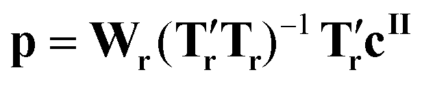
Let us denote mt and ms the number of times and Raman shifts at which the Raman intensity is measured during the kinetic experiment. These data are stored in the matrix M (of size mt × ms). Note that the number of selected Raman shifts should necessarily be smaller than the number of times at which the spectra are recorded. PCA consists in projecting the matrix M onto a score matrix Tr of size mt × mr with mr ≤ ms. Typically, the dimension of the problem is reduced from ms ≈ 102–104 strongly correlated or even linearly dependent variables to mr ≈ 2–10 linearly independent variables, which are linear combinations of the original variables. The matrix of weights (or loadings), which regresses M on Tr is denoted Wr (of size ms × mr) and is defined such that:
| Tr = MWr | (1) |
Note that eqn (1) can be applied to mr = ms, so that the matrices Ts and Ws are of size mt × ms and ms × ms, respectively. The size of the problem can then be reduced to mr < ms simply by defining Tr and Wr as the first mr columns of Ts and Ws, respectively. Once the matrices Wr and Tr have been determined, the matrix M is regressed on the vector cII (of size mt × 1) containing the known concentrations of crystals of form II. This can be mathematically written as:
| cII = Mp | (2) |
 | (3) |
In the case where the data are not passing through the origin, a constant coefficient must be added to eqn (2). This can be implemented by rewriting the equation as follows:
| cII = Nq | (4) |
1.6 Kinetic model
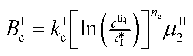
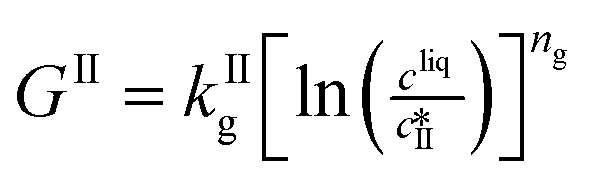
The kinetic model used in this paper accounts for the nucleation and growth of form I as well as for the nucleation, growth and dissolution of form II. The selected expressions of the nucleation (B), growth (G) and dissolution (D) rates are given in Table 1. The supersaturation derives from a difference in chemical potential and is thus best described as the logarithm of the ratio between the actual concentration in the liquid phase (denoted cliq) and the concentration at saturation, i.e., the solubility (denoted and
and  for forms I and II, respectively). A linearization of the dissolution rate was employed because the solute concentration is close to the solubility of form II during the dissolution process.
| Form I | |
|---|---|
| Cross-nucleation |
|
| Secondary nucleation |
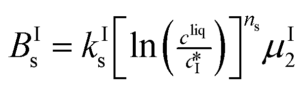
|
| Growth |
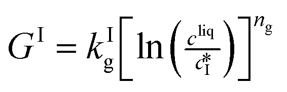
|
| Form II | |
|---|---|
Secondary nucleation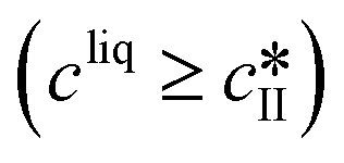 |
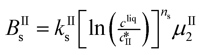
|
Growth |
|
Dissolution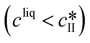 |
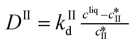
|
The nucleation rates are assumed to be proportional to the second order moment (denoted μ2) of form I or form II depending on the type of nucleation. The second order moment is proportional to the total crystal surface and is defined rigorously later on (see eqn (7) and (8)), while some additional comments on the expression of the nucleation rates are given here. Considering form II first, secondary nucleation is expected to be dominant with respect to primary nucleation since the crystallizer is seeded with crystals of form II. Accordingly, the nucleation rate of form II is considered to be proportional to μII2 (see BIIs in Table 1). Note that such lumped expression is sometimes assumed to average contributions from both primary and secondary nucleation in a coarse-grained manner. On the other hand, it is necessary to explicitly account for the primary nucleation of form I in order to explain its appearance in the crystallizer (setting μI2 = 0 at time 0 would indeed otherwise result in the absence of form I all along the crystallization process). True homogeneous primary nucleation is often considered unrealistic in finite size vessels, so that heterogeneous nucleation on surfaces is regarded as the predominant mechanism of primary nucleation. A surface that is highly likely to promote the nucleation of form I is the surface exposed by crystals of form II. Therefore, the primary nucleation of form I is considered here to be proportional to the surface of crystals of form II (see BIc in Table 1). This phenomenon is referred to as cross-nucleation and has been reported for several systems in the literature, including ROY,26L-glutamic acid,11,14,27D-mannitol,28,29 and polypivalolactone.30 Besides cross-nucleation, form I also appears by secondary nucleation, with an expression similar to that employed for form II (see BIs in Table 1).
In Table 1, the parameters k are temperature dependent rate constants, while the exponents n are assumed to be temperature independent. The indexes c, s, g and d refer to cross-nucleation, secondary nucleation, growth and dissolution, respectively. For the sake of simplicity, it is assumed that ns and ng are identical for the two forms.
In a batch crystallizer, the population balance equations (PBE) describing the time evolution of the concentration of crystals of form I and II are written as follows:
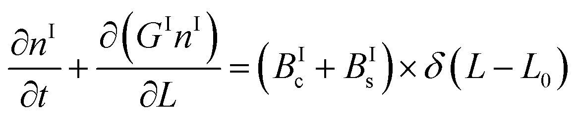 | (5) |
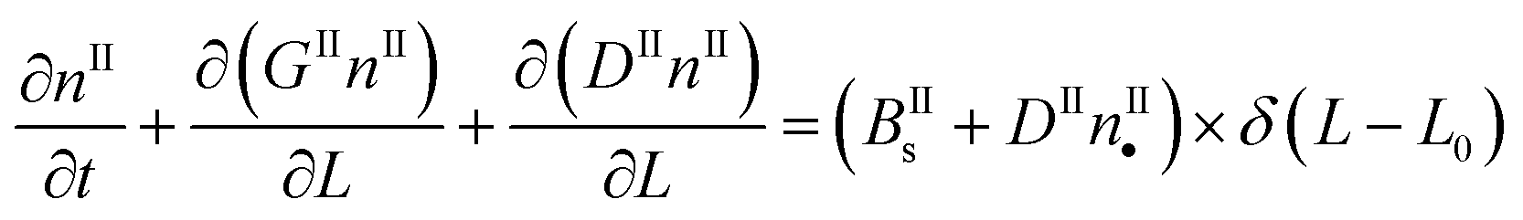 | (6) |
In this work, the PBE were solved by using the methods of moments. The moments of order j of the crystal size distributions of both forms are defined as follows:
μIj = ∫∞0![[thin space (1/6-em)]](https://www.rsc.org/images/entities/char_2009.gif) LjnI(t,L)dL LjnI(t,L)dL | (7) |
| μIIj = ∫∞0LjnII(t,L)dL | (8) |
By applying the above definitions, the PBE given in eqn (5) and (6) are written as:
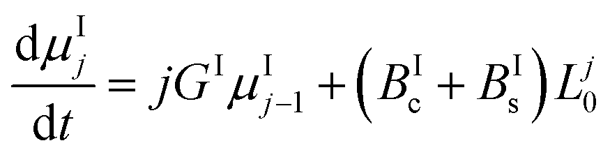 | (9) |
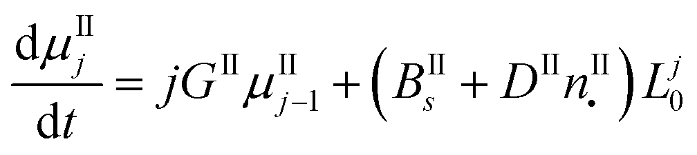 | (10) |
These equations are coupled to a mass balance on the solute:
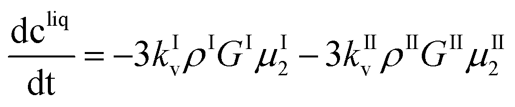 | (11) |
| cI = kIvρIμI3 | (12) |
| cII = kIIvρIIμII3 | (13) |
Eqn (9)–(11) are straightforward to solve in the absence of dissolution. However, when solvent-mediated transformation occurs, it is necessary to estimate nII•, which is not directly obtained from the moment equations. Here, we estimate nII• according to the method employed by Cornel et al.9 This method relies on the reconstruction of the crystal size distribution at the time where dissolution starts by using a Laplace based technique previously derived by Qamar et al.31 Briefly, the idea is to first solve the moment equations until td, the time when dissolution starts, so as to obtain the time dependence of the nucleation and growth rates. Then, the size distribution of crystals of form II at time td can be computed as:
| nII(td,L) = nII0(L − uII(td)) + rII(L) | (14) |
 | (15) |
 | (16) |
 | (17) |
The first term in eqn (14) describes the growth of seeds, while the second one accounts for nucleation and growth of newly formed crystals. Once the size distribution of crystals of form II is computed at the moment where dissolution starts, the concentration of crystals of form II of size L0 at any time t ≥ td can be computed as nII• = nII(t, L = L0) = nII(td, L•), where the length L•(t) is computed by integrating dL•/dt = |DII(t)| with the initial condition L•(t = 0) = L0. Indeed, since dissolution simply shifts the crystal size distribution to lower sizes, it is equivalent to keep L = L0 and increase the time t, or keep t = td and increase the length L• at a rate equal to the dissolution rate.
The moment equations were solved using concentrations in kg of paracetamol per cubic meter of suspension. Density measurements were performed at various concentrations and temperatures to allow the conversion to kg of paracetamol per kg of ethanol. The results of density measurements are presented in the ESI.†
2 Results and discussion
2.1 Solubility
Since solubility dictates the thermodynamics of crystallization, we started our study by estimating the solubility of both forms of paracetamol. The measured solubility values of form I and form II in ethanol are shown as a function of temperature with blue and red circles, respectively, in Fig. 1. These data were described by a thermodynamic model in our previous article.32 Here, we simply fit the experimental data with the following exponential expressions: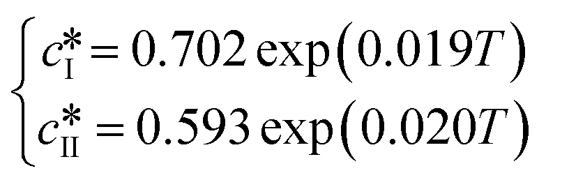 | (18) |
 and
and  are the solubilities of form I and II, respectively, expressed in mg gEtOH−1, while T is the temperature in Kelvin. The results of the fitting are represented by solid lines in Fig. 1.
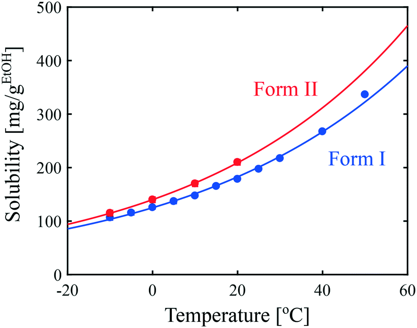 | ||
| Fig. 1 Solubility of paracetamol form I and form II in ethanol as a function of temperature. Symbols represent experimental data and lines correspond to the fits given in eqn (18). | ||
It is seen in Fig. 1 that form I is the most stable over the entire range of temperatures investigated. In addition, the difference in solubility between the two forms decreases at lower temperatures. This suggests that the crystallization of form II is thermodynamically more favored at low temperatures than at high temperatures.
2.2 Calibration of process analytical tools
Process analytical technologies (PAT) are increasingly used for process monitoring and control, both at the laboratory and industrial scales.33 In this work, ATR-FTIR and Raman spectroscopy were used to quantify the solute concentration and the concentration of form II, respectively, as a function of time. The use of such analytical tools requires first proper calibration, whose results are reported in this section.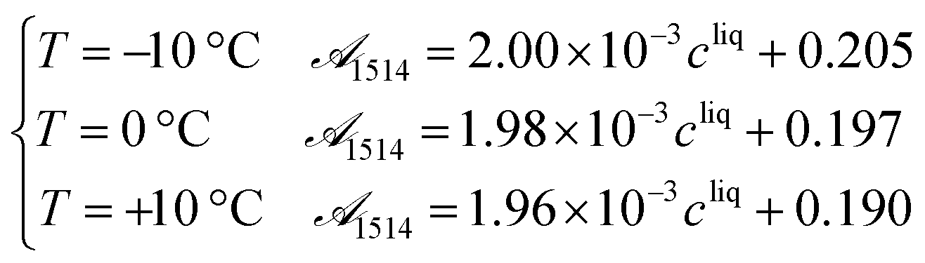 | (19) |
![[scr A, script letter A]](https://www.rsc.org/images/entities/char_e520.gif) 1514 denotes the absorbance at 1514 cm−1 and cliq is the solute concentration in mg gEtOH−1.
1514 denotes the absorbance at 1514 cm−1 and cliq is the solute concentration in mg gEtOH−1.
 | (20) |
As a comparison, the following calibration has been reported previously in the literature: A454/A465 = 482/(100 − fII) − 0.324.36 This expression has the disadvantage to diverge when the percentage of form II tends towards 100%, and eqn (20) was thus preferred.
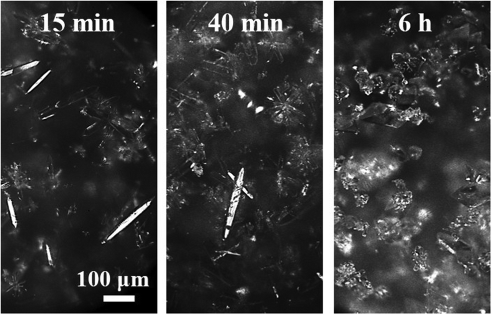 | ||
| Fig. 2 Online images recorded during the seeded crystallization of form II with the following operating conditions: T = 0 °C, cliq0 = 300 mg gEtOH−1, N = 400 rpm. | ||
The Raman spectra at the beginning and at the end of the experiment are shown in the ESI.† Several peaks and peak ratios were tracked as a function of time in an attempt to rationalize the data, i.e., identify some features representing the increase in solid content and change in solid composition. However, such simple analysis was largely unsuccessful.
Exploratory data analysis can provide useful qualitative information on the main characteristics of online measurements. Here, principal component analysis (PCA) was performed on the online Raman data and the results are shown in Fig. 3. It is usually recommended to pre-process the spectra before applying statistical analysis in order to reduce the effects unrelated to the property of interest (e.g., slight fluorescence and laser fluctuations), so that pertinent changes can be better observed. Various pre-processing approaches have been used in the literature, such as the normalization, smoothing or computation of derivatives of experimental spectra.40,41 The results of Fig. 3 were obtained considering first derivatives (D1) followed by standard normal variate (SNV) treatment. The latter correction consists in subtracting the mean of the spectrum and subsequently dividing it by the standard deviation. Fig. 3(a) shows the scores of the first four principal components as a function of time together with the explained percentage of variance. It is generally difficult to relate principal components to physical quantities. Nevertheless, it is seen that the trend of the first principal component (PC1) somehow resembles the expected trend of the concentration of crystals of form II: it increases due to crystallization, reaches a maximum, and then decreases due to transformation into form I. On the other hand, the trend of the second principal component (PC2) is not too far from the expected trend of the concentration in the liquid phase, with a sharp decrease at the beginning followed by a quite long plateau due to the transformation. In addition, it is seen that the first three principal components describe most of the variance (94.04%), so that PCA allows reducing the size of the system from 1800 recorded wavelengths to 3 principal components. The scores are plotted as a function of the three first principal components in Fig. 3(b). In this graph, each symbol represents a different time point and the arrows indicate the time direction. This representation allows the identification of three phases, denoted ①, ②, and ③, further discussed later on.
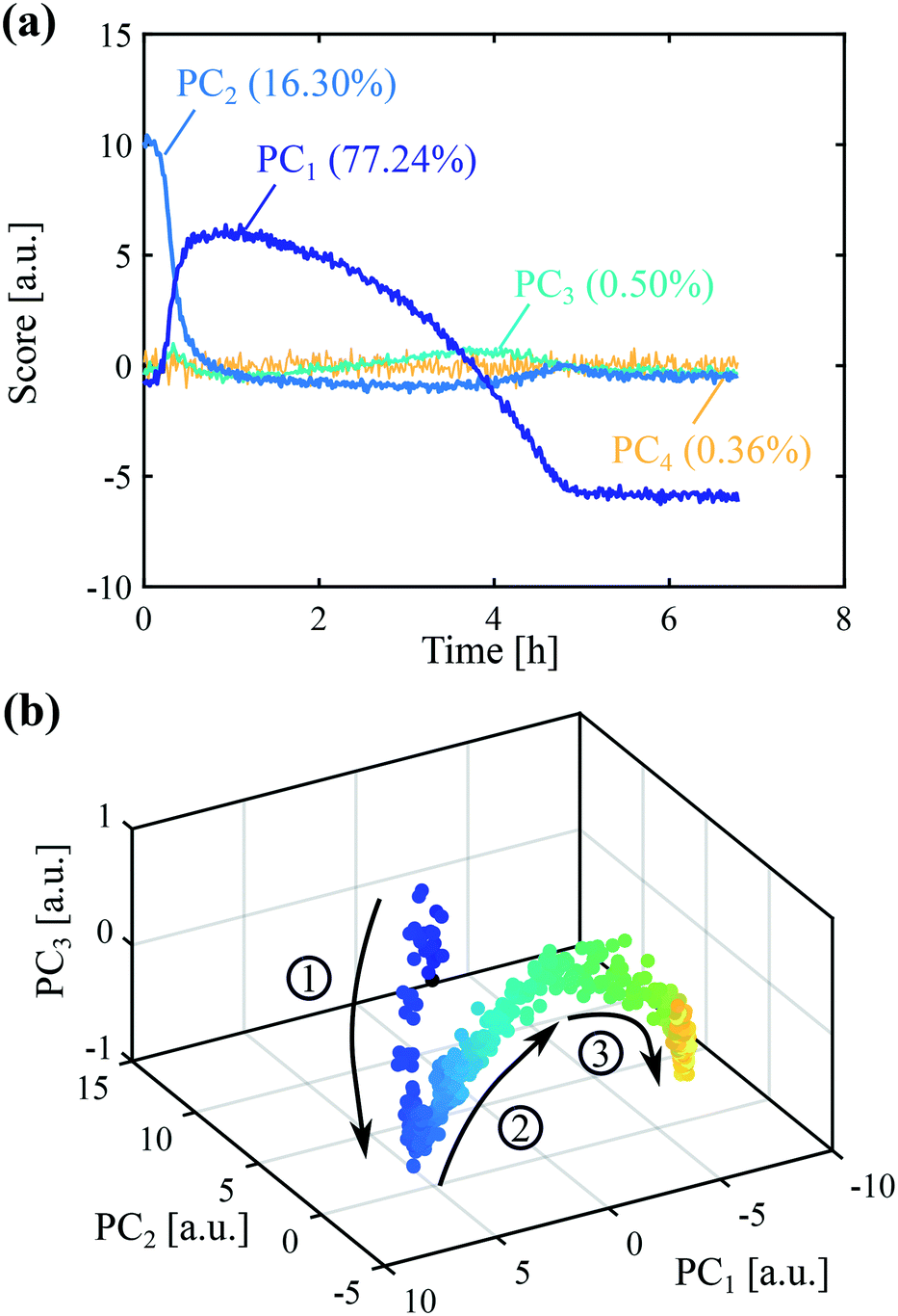 | ||
| Fig. 3 Principal component analysis on a seeded crystallization experiment. The following operating conditions were employed: T = 0 °C, cliq0 = 300 mg gEtOH−1, N = 400 rpm. (a) Scores of the first four principal components as a function of time together with their percentage of explained variance. (b) Scores over time in a three dimensional representation. Arrows indicate the time direction. | ||
After principal component analysis, the online Raman data were regressed with a multilinear model on the concentration of form II determined independently from online ATR-FTIR and offline Raman data. While online ATR-FTIR provides an estimate of the solute concentration (and thus of the total solid concentration by difference), offline Raman measurements provide an estimate of the fraction of form II in dried solid samples. The combination of the two techniques therefore allows assessing the absolute concentration of crystals of form II. The regression vector was determined by PCR, as described in section 1.5.4. The quality of the regression can be appreciated in Fig. 4(a), where the online data are represented by dots and offline data by circles. Two pre-processing methods have been employed, namely SNV (purple dots) and first derivatives followed by SNV (red dots). It can be seen that a good regression can be obtained in both cases.
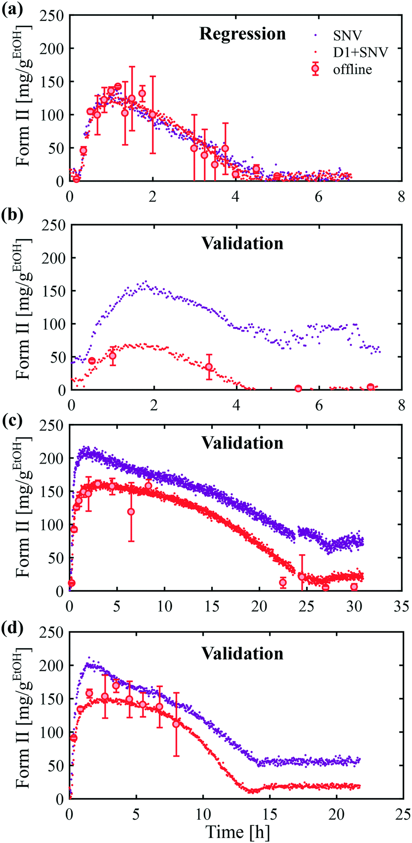 | ||
| Fig. 4 Online Raman calibration. (a) Regression experiment performed with the following operating parameters: cliq0 = 300 mg gEtOH−1, T = 0 °C, N = 400 rpm (b–d) validation experiments. In each case, only one parameter was varied, namely: (b) cliq0 = 250 mg gEtOH−1, (c) T = −10 °C, (d) N = 300 rpm. | ||
Then, the validity of the calibration was assessed by its ability to determine the concentration of form II in other conditions. To do so, three validation experiments were performed, where in each of them one operating parameter was varied as compared to the regression experiment. The results are presented in Fig. 4(b–d). In panel (b), the concentration was decreased from 300 mg gEtOH−1 to 250 mg gEtOH−1. In panel (c), the temperature was decreased from 0 °C to −10 °C. In panel (d), the stirring speed was decreased from 400 rpm to 300 rpm. In each case, the same two pre-processing methods as those used for the regression, namely SNV and first derivative followed by SNV, were tested. It is seen that the calculations of the online concentration of form II are in very good agreement with the offline measurements in the case where the signals were pre-processed using the first derivatives followed by SNV. As a comparison, the calculations are less accurate when using SNV alone. Therefore, the method of first derivatives combined with SNV was selected to analyze subsequent data. The results of Fig. 4 validate the statistical model used to process online Raman data.
2.3 Crystallization kinetics
Batch crystallization experiments were performed in ethanol at various concentrations (from 250 mg gEtOH−1 to 300 mg gEtOH−1), various temperatures (from −10 °C to +10 °C), and various stirring speeds (from 200 rpm to 400 rpm). In each case, the crystallizer was seeded with crystals of form II. Experimental results are presented with dots in Fig. 5. The concentration of paracetamol in the liquid phase was determined by online ATR-FTIR and is shown in black. The concentration of crystals of form II was determined by online Raman spectroscopy using the multilinear model described in the previous section and is shown in red. Finally, the concentration of crystals of form I was determined by a mass balance knowing the initial concentration, the solute concentration and the concentration of crystals of form II, and is shown in blue.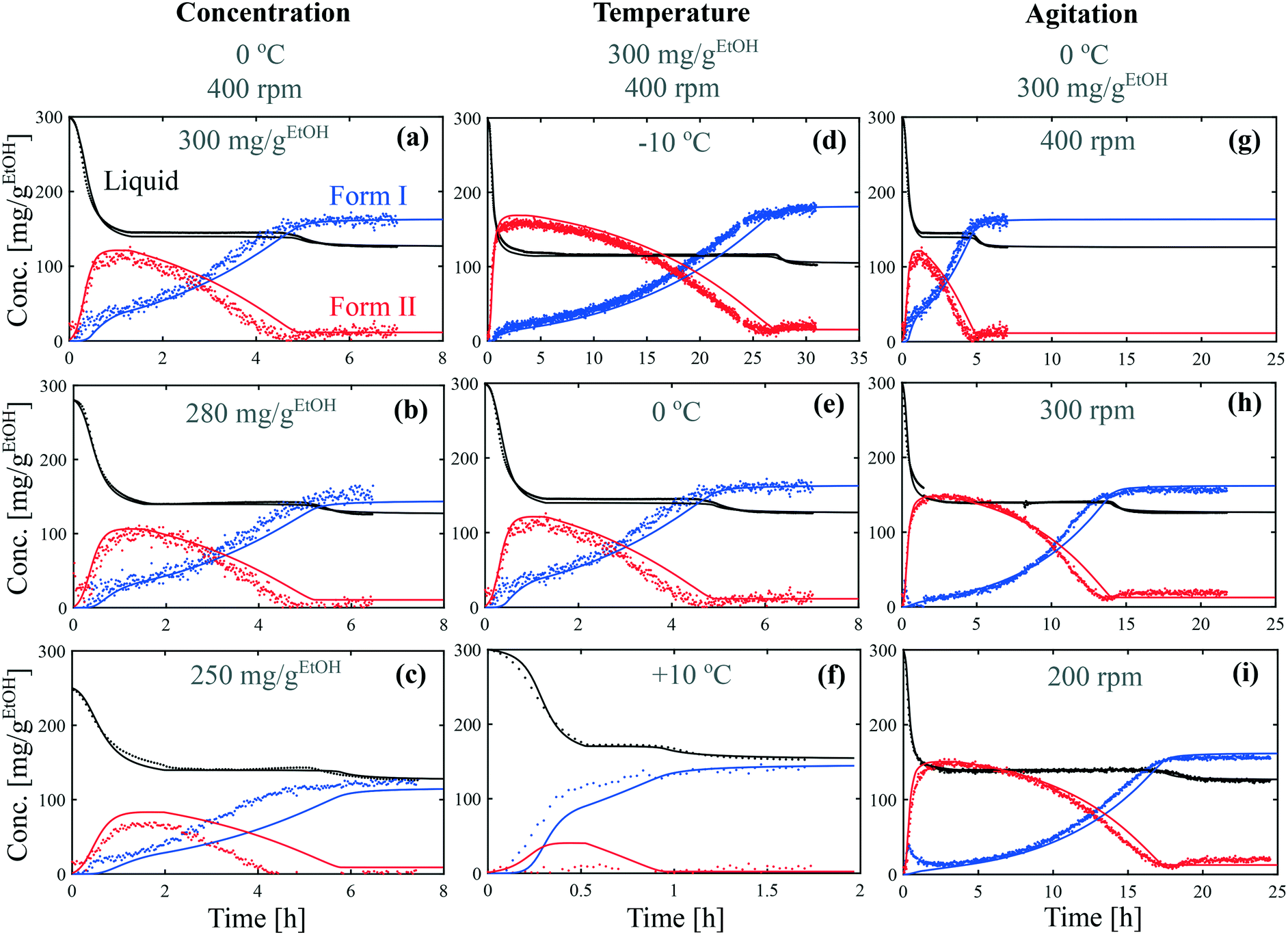 | ||
| Fig. 5 Crystallization kinetic experiments under various conditions of (a–c) concentration, (d and e) temperature and, (g–i) agitation speed. Experimental data are represented by dots and model simulations by lines. The concentrations of dissolved paracetamol, crystals of form I, and crystals of form II are show in black, blue, and red, respectively. The model parameters are summarized in Fig. 6 and 7. | ||
Although the time frame of crystallization varies greatly between the different conditions, all the experiments share common features, with three distinct phases. During the first phase, the concentration in the liquid phase drops due to the crystallization of form II (in parallel to the crystallization of form I in some cases). Then, the crystals of form II dissolve and recrystallize as form I. During this transformation, the concentration in the liquid phase stays constant at the solubility of form II. Finally, the concentration in the liquid phase drops toward the solubility of form I due to the further crystallization of form I. These three phases correspond to the phases ①, ②, and ③ identified in Fig. 3(b).
The data presented in Fig. 5(a) correspond to a repetition of the experiment presented in Fig. 4, and thus show the good reproducibility of the experiments. It is seen in Fig. 5(a–c) that a decrease in the initial solute concentration from 300 mg gEtOH−1 to 250 mg gEtOH−1 slows down phase ①, i.e., it takes more time to reach the solubility of form II. This is due to a decrease in the supersaturation. In addition, it is observed that for each concentration, after 1 h of cooling (i.e., approximately when cliq approaches  ), the fraction of form II exceeds 60%. This suggests that the initial concentration has only a weak impact on the polymorphic content.
Considering now the data shown in Fig. 5(d–f), it is seen that temperature has a very strong impact, not only on the time scale of the experiment (from 1.5 h at +10 °C to 30 h at −10 °C), but also on the polymorphic content. In particular, form II can be obtained at a decent concentration only at −10 °C and 0 °C. At +10 °C, the crystallization of form I is so fast that seeding is not sufficient to induce the crystallization of form II. It is already anticipated from these data that the differences in solubility reported in Fig. 1 cannot explain such drastic changes in the polymorphic outcome. A more detailed kinetic analysis is performed in the next section.
Finally, the results shown in Fig. 5(g–i) indicate that the stirring speed has a negligible influence on the kinetics of crystallization of form II, but has a strong influence on the kinetics of transformation. Indeed, no substantial differences are noticed in the solute depletion kinetics at the beginning of the experiment, but a significantly longer plateau is observed when decreasing the stirring speed from 400 rpm to 200 rpm. In addition, a higher concentration of form II is reached at lower stirring speeds.
2.4 Model parameters estimation
In this section, we describe the experimental data of Fig. 5 with the kinetic model presented in section 1.6, which accounts for the primary (cross) nucleation, secondary nucleation, and growth of form I, as well as the secondary nucleation, growth and dissolution of form II. The implementation of the model requires first to estimate model parameters.For the sake of simplicity, it was assumed that both polymorphs have the same density, which was set here to ρI = ρII = 1332 kg m−3 in agreement with previous publications.34,42,43 The shape factor of form I has been estimated to kIv = 0.866 in the literature.44 On the other hand, the shape factor of form II has been estimated in this work to kIIv ≈ 2. To do so, a simplified morphology based on the one reported in the literature45 has been considered and pictures were analyzed to determine the length, width and thickness of a number of crystals of form II. The width was chosen as the characteristic length L, and the shape factor was estimated from the measurement of the crystal volume as V = kvL3. More details about the calculation of the crystal volume as a function of the crystal width for the selected morphology are given in the ESI.†
The seed size distribution was described by a gamma distribution of average size and standard deviation equal to 120 μm and 70 μm, respectively. The comparison between the experimental seed distribution estimated from online images and the fitted distribution is given in the ESI.†
The parameters ns and ng were set to 3 and 2, respectively, so as to obtain a concentration dependence of the secondary nucleation rate and growth rate of form I in reasonable agreement with previous works.34,43,44,46 In the absence of data on the cross-nucleation of form I over form II, several values of nc ranging from 2 to 4 were tested. It was found that nc = 2 describes best the experimental data.
The kinetic parameters kIc, kIs, kIg, kIIs, kIIg, and kIId were determined by fitting model simulations to the experimental results obtained at the stirring speed of 400 rpm. For each temperature, at least two initial concentrations were considered. This corresponds to the data shown in Fig. 5(a–f) and in Fig. S11 of the ESI† (results at 250 mg gEtOH−1 at −10 °C and +10 °C). The optimization procedure relied on the minimization of the sum of squared residuals with a genetic algorithm. The squared residuals of the solute concentration were multiplied by a factor 100 with respect to the squared residuals of the concentration of form II in order to obtain similar errors for both quantities. The model simulations are represented with solid lines in Fig. 5(a–f) and in Fig. S11 of the ESI,† showing a good agreement with the experimental data.
The parameters obtained for the reference case of T = 0 °C and N = 400 rpm are presented in Table 2. For each kinetic parameter, the reported confidence interval corresponds to the range over which the considered parameter can be varied while leading to a change in the error function by less than 10% (keeping all the other parameters constant). It is observed that the growth rate constants are the parameters having the smallest confidence intervals, then come the nucleation rate constants and finally the dissolution rate constant. The latter is difficult to estimate with accuracy because the polymorphic transformation of the investigated system is not limited by dissolution. In other words, any value of kIId larger than a certain threshold ensures a satisfactory description of the experimental data. The crystallization of form II paracetamol from ethanolic solutions has already been reported,47,48 but to the best of our knowledge, no kinetic parameters related to the nucleation, growth and dissolution of form II are available to date in the literature. Nevertheless, the crystallization kinetics of form I has been studied by several authors.34,43,44,46 A comparison between the secondary nucleation and growth rates obtained in this work and those obtained in the aforementioned citations is provided in the ESI.† The secondary nucleation rates obtained in the various studies span considerably different orders of magnitude, and the results obtained in this work fall in between the lowest and highest reported estimates. On the other hand, the data on the growth rates are quite consistent between the different works, this one included.
| Form I | Form II | ||
|---|---|---|---|
| n c | [—] | 2 | n.a. |
| k c | [# m−3 min] | (1.37 ± 0.13) × 107 | n.a. |
| n s | [—] | 3 | 3 |
| k s | [# m−2 min] | (7.17 ± 0.23) × 109 | (1.50 ± 0.17) × 107 |
| n g | [—] | 2 | 2 |
| k g | [m min−1] | (1.04 ± 0.01) × 10−5 | (5.22 ± 0.07) × 10−5 |
| k d | [m min−1] | n.a. | (5.42 ± 3.04) × 10−4 |
The temperature dependence of kIc, kIs, kIg, kIIs, kIIg, and kIId can be assessed in Fig. 6. Those data were regressed with an Arrhenius model of the type k = k0exp(−Ea/RT), where k0 is a prefactor, Ea the activation energy, and R the ideal gas constant. The values of k0 and Ea for the nucleation, growth and dissolution rate constants are summarized in Table 3. As mentioned previously, the data on the nucleation of form I are quite scattered in the literature. However, three separate studies report similar values of the activation energy of the growth of form I, namely around 41 kJ mol−1.34,44,46 To compare the present results with those of these previous studies, it is first necessary to unify the definition of the reaction rates. Here, the reaction rates are written as:
 | (21) |
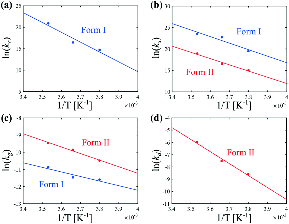 | ||
| Fig. 6 Arrhenius dependence of the kinetic rate constants of (a) cross-nucleation, (b) secondary nucleation, (c) growth, and (d) dissolution at 400 rpm. | ||
| Form I | Form II | |||
|---|---|---|---|---|
| k c | k 0 | [# m−3 min] | 1.16 × 1044 | n.a. |
| E a | [kJ mol−1] | 191 | n.a. | |
| k s | k 0 | [# m−2 min] | 5.62 × 1033 | 2.53 × 1030 |
| E a | [kJ mol−1] | 127 | 121 | |
| k g | k 0 | [m min−1] | 0.21 | 62.7 |
| E a | [kJ mol−1] | 22.2 | 31.9 | |
| k d | k 0 | [m min−1] | n.a. | 2.34 × 10¹² |
| E a | [kJ mol−1] | n.a. | 81.4 |
A different expression of the supersaturation was selected in previous works, so that the growth rates were written as:34,44,46
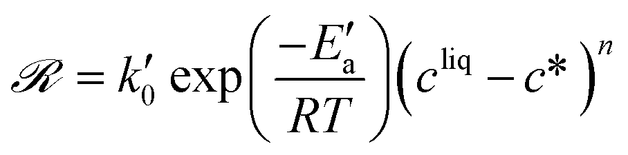 | (22) |
By approximating ln(cliq/c*) to (cliq − c*)/c*, one obtains:
 | (23) |
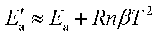
exp(βT). By adapting eqn (18) (in mg gEtOH−1) to the proper units (kg m−3), we obtain β = 0.016. With n = 2, Ea = 22.2 kJ mol−1 and T = 0 °C, it results that the activation energy of the growth of form I is in the order of 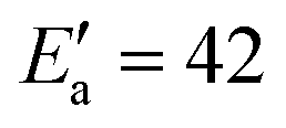 kJ mol−1, which is in very good agreement with the value reported in previous works.
The data shown in Fig. 6 allow shedding light on the experimental observation that the crystallization of form II is favored at low temperatures (see Fig. 5). It is in fact seen in Fig. 6 that the primary (cross) nucleation of form I is strongly reduced at low temperatures. On the other hand, it seems that temperature affects the secondary nucleation and growth rates of forms I and II in a relatively similar way. Therefore, the inhibition of the crystallization of form I with respect to form II under cold conditions cannot be explained by a change in the ratios kIs/kIIs or kIg/kIIg. Overall, the improvement in the content of form II at low temperatures is attributed to a decrease in the primary nucleation rate of form I. Note that for the sake of simplicity, the primary nucleation rate was considered here to be proportional to the surface of crystals of form II only, and was thus referred to as cross-nucleation. Nevertheless, the estimated kinetic constants rather correspond to lumped values considering all primary nucleation phenomena taken together, including cross-nucleation, but also homogeneous nucleation and heterogeneous nucleation on the surfaces present in the crystallizer (e.g., walls of the vessel, impeller, probes).
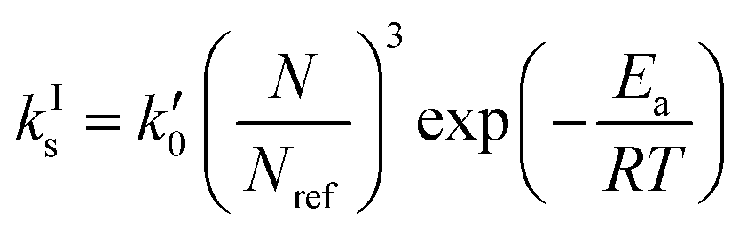
Let us now focus on the impact of the stirring speed. It was observed in Fig. 5(g–i) that a decrease in the stirring speed has a negligible impact on the decrease in the solute concentration before it reaches the solubility of form II, but significantly increases the length of the plateau at the solubility of form II. This suggests that the stirring speed has a weak impact on the crystallization of form II, but significantly delays the formation of form I. Accordingly, the parameters kIIs and kIIg were kept unchanged at all stirring speeds. Under such vigorous stirring, it is unlikely that growth and dissolution are diffusion limited, so that kIg and kIId can also reasonably be considered independent of the stirring speed. Overall, a change in the stirring speed is expected to impact kIc and/or kIs. For the sake of simplicity, it was assumed that only kIs is impacted by the stirring speed. The fitted values of kIs are plotted as a function of N in Fig. 7 (symbols), while the quality of the fitting can be appreciated in Fig. 5(g–i). It is seen that the experimental data acquired between 200 rpm and 400 rpm can be well explained by a change in kIs only. The trend of kIs with N can be described by the following empirical expression: kIs = 106N3, which is represented by a solid line in Fig. 7. Therefore, the effect of temperature and agitation speed on kIs can be accounted for simultaneously using the following lumped expression:
 | (24) |
 = 8.6 × 1025 # m−2 min and Ea = 127 kJ mol−1. The reference stirring speed Nref is set to 1 rpm so as to have kIs and
  in the same units.
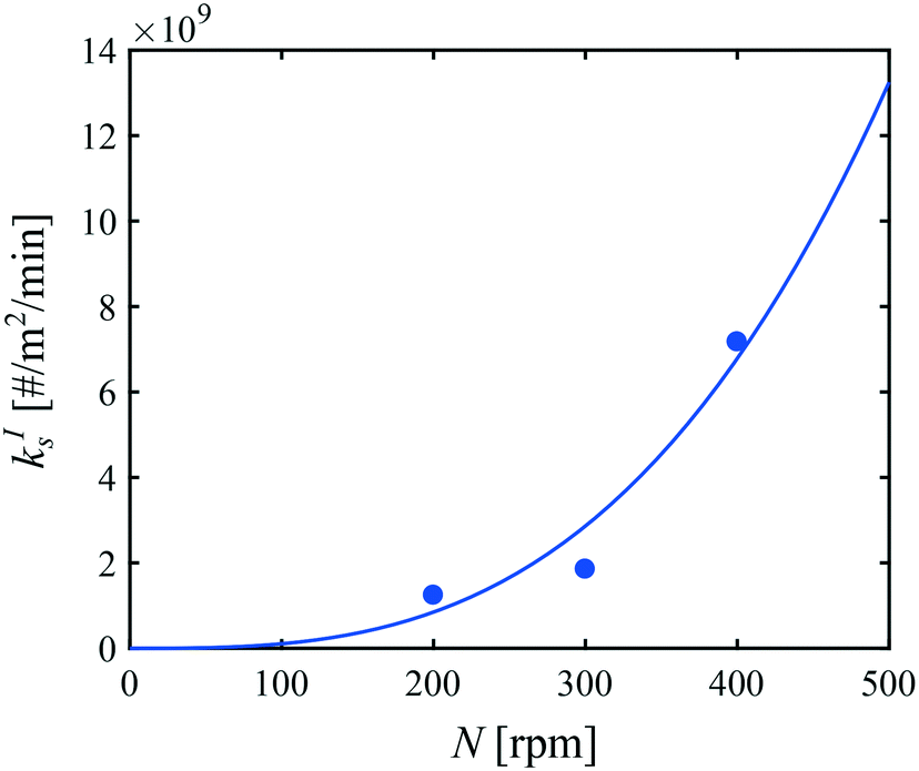 | ||
| Fig. 7 Impact of the agitation speed on the secondary nucleation rate constant of form I at 0 °C. Symbols correspond to fitted values of kIs, while the line represents the following empirical expression kIs = 106N3. | ||
2.5 Process performance parameters
The kinetic model developed in the previous section can now be used to select the operating conditions allowing the production of form II within some target specifications in terms of polymorphic purity, yield, and productivity. These three process performance parameters are defined as follows:Polymorphic purity: mass of form II over total mass of crystals
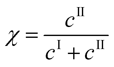 | (25) |
Yield: produced mass of form II over total mass of paracetamol
 | (26) |
Productivity: mass of crystals per unit volume and unit time
 | (27) |
The impact of concentration, temperature, and agitation on the polymorphic purity, yield, and productivity is analyzed in Fig. 8. Let us start with Fig. 8(a), which shows the yield as a function of the polymorphic purity for various initial concentrations. For each of these curves, at time 0, the polymorphic purity is equal to 100% and the yield to 0% because it corresponds to the presence of the seeds only. When time passes, crystals are formed, the yield increases, but the polymorphic purity decreases due to the crystallization of form I. When the yield is maximum, the solubility of form II is reached. Later on, the yield decreases due to solvent-mediated transformation. Therefore, crystals should be harvested before the yield starts decreasing, which means that only the right part of the curves shown in Fig. 8 should be considered for process design. It is observed in Fig. 8(a) that an increase in the initial concentration leads to an increase in the yield. To understand this observation, let us introduce the theoretical yield defined as follows:
 | (28) |
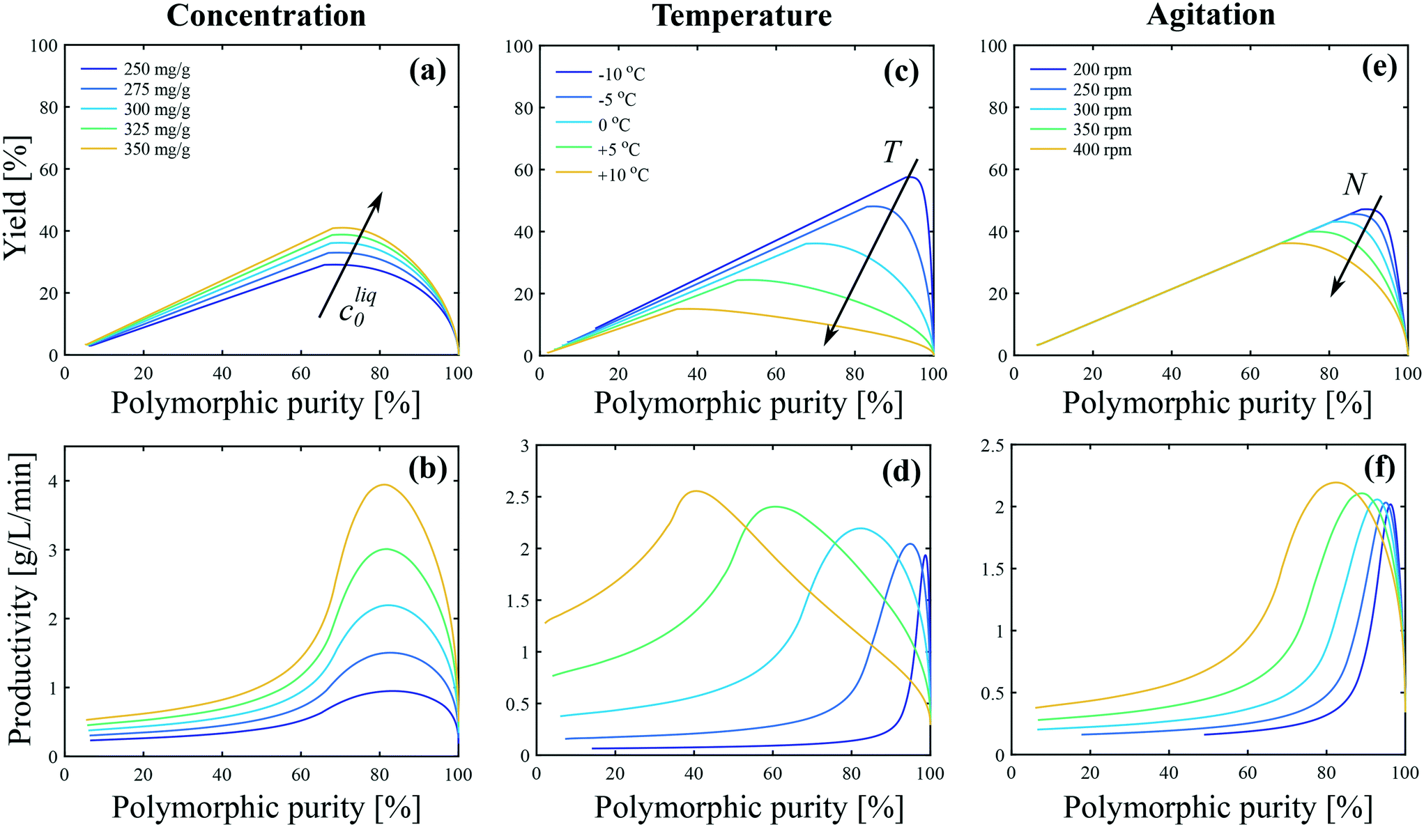 | ||
| Fig. 8 Impact of (a and b) concentration, (c and d) temperature, and (e and f) agitation on the polymorphic purity, yield and productivity. The process performance parameters are defined with respect to form II as shown in eqn (25)–(27). In panels (a and b) T = 0 °C and N = 400 rpm. In panels (c and d) cliq0 = 300 mg gEtOH−1 and N = 400 rpm. In panels (e and f) T = 0 °C and cliq0 = 300 mg gEtOH−1. | ||
The theoretical yield corresponds to the “best possible yield”, i.e., the yield that would be obtained if form II could be crystallized at 100% purity when the solute concentration reaches the solubility of form II. When the initial concentration is increased from 250 mg gEtOH−1 to 350 mg gEtOH−1, the theoretical yield increases from 44% to 60%. On the other hand, the maximum achievable yield increases from 29% to 41% (see Fig. 8(a)), so that ϑ/ϑ* increases from approximately 66% to 68%. This is better shown in Fig. S13(a) of the ESI,† where the ratio ϑ/ϑ* is plotted as a function of the polymorphic purity. It is seen that the curves obtained at various initial concentrations all overlap on one single curve. This indicates that the improvement in the yield–purity trade-off observed in Fig. 8(a) at higher concentration is mainly due to an increase in the theoretical yield. Considering now Fig. 8(b), the productivity starts at 0 (when the polymorphic purity is 100%) and increases due to the formation of crystals. When the solubility of form II is reached, solution-mediated transformation starts. No more crystals are produced and the productivity becomes inversely proportional to time. It is observed in Fig. 8(b) that an increase in cliq0 leads to an increase in productivity. This is because, for a given reactor volume, productivity is directly proportional to the concentration of crystals produced.
Let us now focus on the impact of temperature. It is observed in Fig. 8(c) that temperature has a strong impact on the yield–purity trade-off. Indeed, it is possible to obtain simultaneously a high yield and a high polymorphic purity only at low temperatures. For instance, if a polymorphic purity of 95% is targeted, the yield at +10 °C is only in the order of 5%, whereas it is around 60% at −10 °C. When the temperature is decreased from +10 °C to −10 °C, the theoretical yield increases from 43% to 62%. On the other hand, the maximum achievable yield increases from 15% to 58% (Fig. 8(b)). Consequently, the ratio ϑ/ϑ* increases from 35% to 93% when decreasing the temperature from +10 °C to −10 °C. This is further illustrated in Fig. S13(b) of the ESI,† where the ratio ϑ/ϑ* is plotted as a function of the polymorphic purity for various temperatures. The improvement in the yield–purity trade-off observed in Fig. 8(c) at low temperatures is thus mainly due to the inhibition of primary nucleation of form I (and also to an increase in the theoretical yield). However, such improvement of the yield comes at the expense of a lower productivity because lower temperatures are associated with slower kinetics. This is illustrated in Fig. 8(d), where it is seen that the productivity maximum decreases when the temperature is decreased. In addition, very cold temperatures may be difficult to achieve in large scale crystallizers and are energy intensive.
Finally, the impact of agitation can be appreciated in Fig. 8(e and f). It is observed that, for a given target purity, a higher yield is obtained at low stirring speed. This is due to the inhibition of the crystallization of form I with respect to form II at lower stirring speeds. Nevertheless, a sufficient stirring speed should be selected in order to keep the crystals suspended and ensure a good mass/heat transfer.
It is evident from Fig. 8 that all process performance parameters (i.e., polymorphic purity, yield, and productivity) cannot be maximized simultaneously. Therefore, depending on the process specifications, different operating conditions should be selected. This is illustrated in Fig. 9, where the productivity is plotted as a function of the temperature for different values of the target polymorphic purity. For instance, it is seen that if a rather low polymorphic purity is acceptable (e.g., 80%), the productivity goes through a maximum as a function of temperature, and the most productive process is obtained at around 0 °C. On the other hand, if a very high polymorphic purity is requested (e.g., 98%) and the process is still operated at 0 °C, the crystallization should be stopped prematurely to satisfy the purity constraint, which would lead to a low productivity. Therefore, if a high polymorphic purity is targeted, it is necessary to run the process at very low temperatures, in the order of −10 °C. These results illustrate how process modeling can help selecting the most appropriate operating conditions for a given system.
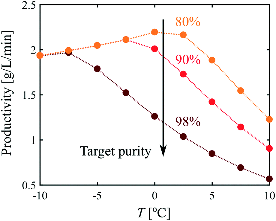 | ||
| Fig. 9 productivity as a function of temperature for different target purity values. | ||
3 Conclusions
In this work, we investigated polymorph dynamics in seeded batch crystallizers considering the cooling crystallization of paracetamol form II as a case study. The solute concentration and the polymorphic content were monitored with online ATR-FTIR and online Raman spectroscopy, respectively. A proper calibration of the Raman signal could be obtained by applying principal component regression on only one kinetic experiment, where form II crystallizes and then transforms into form I. A suitable pre-processing treatment of the spectra was found necessary to obtain a satisfactory calibration.Experimental characterization was complemented by population balance modeling considering the primary (cross) nucleation, secondary nucleation, and growth of form I, as well as the secondary nucleation, growth, and dissolution of form II. It was found that low temperatures and low agitation speeds promote the crystallization of form II with respect to form I due to a decrease in the nucleation rate of form I. In particular, it was observed that at temperatures above approximately 0 °C, seeding the crystallizer with crystals of form II is not sufficient to induce the crystallization of form II.
The impact of operating conditions (concentration, temperature, stirring speed) on process performance parameters (polymorphic purity, yield, productivity) was investigated. It was shown that the temperature leading to the most productive process strongly depends on the target polymorphic purity. This work illustrates how the combination of experimental characterization with mechanistic modeling allows gaining a deep understanding of the crystallization process and selecting the most suited operating conditions to satisfy certain process requirements.
Conflicts of interest
There are no conflicts to declare.Acknowledgements
Financial support from the Swiss National Science Foundation is gratefully acknowledged (grant P2EZP2_168909). We thank Richard Becker for interesting discussions and valuable technical support.References
- H. G. Brittain, Polymorphism in pharmaceutical solids, CRC Press, 2016 Search PubMed.
- A. Y. Lee, D. Erdemir and A. S. Myerson, Annu. Rev. Chem. Biomol. Eng., 2011, 2, 259–280 CrossRef CAS PubMed.
- E. H. Lee, Asian J. Pharm. Sci., 2014, 9, 163–175 CrossRef.
- M. Kitamura, CrystEngComm, 2009, 11, 949–964 RSC.
- A. Llinàs and J. M. Goodman, Drug Discovery Today, 2008, 13, 198–210 CrossRef PubMed.
- D. Mangin, F. Puel and S. Veesler, Org. Process Res. Dev., 2009, 13, 1241–1253 CrossRef CAS.
- Z. Yu, J. Chew, P. Chow and R. Tan, Chem. Eng. Res. Des., 2007, 85, 893–905 CrossRef CAS.
- J. F. B. Black, P. T. Cardew, A. J. Cruz-Cabeza, R. J. Davey, S. E. Gilks and R. A. Sullivan, CrystEngComm, 2018, 20, 768–776 RSC.
- J. Cornel, P. Kidambi and M. Mazzotti, Ind. Eng. Chem. Res., 2010, 49, 5854–5862 CrossRef CAS.
- J. Cornel, C. Lindenberg and M. Mazzotti, Ind. Eng. Chem. Res., 2008, 47, 4870–4882 CrossRef CAS.
- J. Schöll, D. Bonalumi, L. Vicum, M. Mazzotti and M. Müller, Cryst. Growth Des., 2006, 6, 881–891 CrossRef.
- R. Davey, N. Blagden, S. Righini, H. Alison and E. Ferrari, J. Phys. Chem. B, 2002, 106, 1954–1959 CrossRef CAS.
- K. Sato, J. Phys. D: Appl. Phys., 1993, 26, B77 CrossRef CAS.
- E. S. Ferrari and R. J. Davey, Cryst. Growth Des., 2004, 4, 1061–1068 CrossRef CAS.
- C. Gu, V. Young Jr and D. J. Grant, J. Pharm. Sci., 2001, 90, 1878–1890 CrossRef CAS PubMed.
- N. Guo, B. Hou, N. Wang, Y. Xiao, J. Huang, Y. Guo, S. Zong and H. Hao, J. Pharm. Sci., 2018, 107, 344–352 CrossRef CAS PubMed.
- G. Févotte, A. Caillet and N. Sheibat-Othman, AIChE J., 2007, 53, 2578–2589 CrossRef.
- W. Beckmann, Org. Process Res. Dev., 2000, 4, 372–383 CrossRef CAS.
- M. Müller, U. Meier, D. Wieckhusen, R. Beck, S. Pfeffer-Hennig and R. Schneeberger, Cryst. Growth Des., 2006, 6, 946–954 CrossRef.
- J. Bauer, S. Spanton, R. Henry, J. Quick, W. Dziki, W. Porter and J. Morris, Pharm. Res., 2001, 18, 859–866 CrossRef CAS.
- P. Di Martino, A. Guyot-Hermann, P. Conflant, M. Drache and J. Guyot, Int. J. Pharm., 1996, 128, 1–8 CrossRef.
- E. Joiris, P. Di Martino, C. Berneron, A. M. Guyot-Hermann and J. C. Guyot, Pharm. Res., 1998, 15, 1122–1130 CrossRef CAS.
- P. Di Martino, P. Conflant, M. Drache, J.-P. Huvenne and A.-M. Guyot-Hermann, J. Therm. Anal., 1997, 48, 447–458 CrossRef CAS.
- S. J. Smith, M. M. Bishop, J. M. Montgomery, T. P. Hamilton and Y. K. Vohra, J. Phys. Chem. A, 2014, 118, 6068–6077 CrossRef CAS PubMed.
- L. R. Agnew, D. L. Cruickshank, T. McGlone and C. C. Wilson, Chem. Commun., 2016, 52, 7368–7371 RSC.
- S. Chen, H. Xi and L. Yu, J. Am. Chem. Soc., 2005, 127, 17439–17444 CrossRef CAS PubMed.
- C. Cashell, D. Corcoran and B. Hodnett, Chem. Commun., 2003, 374–375 RSC.
- J. Tao and L. Yu, J. Phys. Chem. B, 2006, 110, 7098–7101 CrossRef CAS PubMed.
- J. Tao, K. J. Jones and L. Yu, Cryst. Growth Des., 2007, 7, 2410–2414 CrossRef CAS.
- D. Cavallo, F. Galli, L. Yu and G. C. Alfonso, Cryst. Growth Des., 2017, 17, 2639–2645 CrossRef CAS.
- S. Qamar, G. Warnecke, M. P. Elsner and A. Seidel-Morgenstern, Chem. Eng. Sci., 2008, 63, 2233–2240 CrossRef CAS.
- L. Nicoud, F. Licordari and A. S. Myerson, Cryst. Growth Des., 2018 DOI:10.1021/acs.cgd.8b01200.
- L. L. Simon, H. Pataki, G. Marosi, F. Meemken, K. Hungerbühler, A. Baiker, S. Tummala, B. Glennon, M. Kuentz and G. Steele, Org. Process Res. Dev., 2015, 19, 3–62 CrossRef CAS.
- N. A. Mitchell, C. T. Ó'Ciardhá and P. J. Frawley, J. Cryst. Growth, 2011, 328, 39–49 CrossRef CAS.
- A. Maher, Ã. C. Rasmuson, D. M. Croker and B. K. Hodnett, J. Chem. Eng. Data, 2012, 57, 3525–3531 CrossRef CAS.
- N. Al-Zoubi, J. Koundourellis and S. Malamataris, J. Pharm. Biomed. Anal., 2002, 29, 459–467 CrossRef CAS PubMed.
- C. Starbuck, A. Spartalis, L. Wai, J. Wang, P. Fernandez, C. M. Lindemann, G. X. Zhou and Z. Ge, Cryst. Growth Des., 2002, 2, 515–522 CrossRef CAS.
- G. Févotte, Chem. Eng. Res. Des., 2007, 85, 906–920 CrossRef.
- E. Simone, A. Saleemi and Z. Nagy, Chem. Eng. Res. Des., 2014, 92, 594–611 CrossRef CAS.
- Å. Rinnan, F. van den Berg and S. B. Engelsen, TrAC, Trends Anal. Chem., 2009, 28, 1201–1222 CrossRef.
- J. Huang, S. Romero-Torres and M. Moshgbar, Am. Pharm. Rev., 2010, 13, 116 CAS.
- T. Vetter, C. L. Burcham and M. F. Doherty, Chem. Eng. Sci., 2014, 106, 167–180 CrossRef CAS.
- P. J. Frawley, N. A. Mitchell, C. T. Ó'Ciardha and K. W. Hutton, Chem. Eng. Sci., 2012, 75, 183–197 CrossRef CAS.
- J. Worlitschek and M. Mazzotti, Cryst. Growth Des., 2004, 4, 891–903 CrossRef CAS.
- G. Nichols and C. S. Frampton, J. Pharm. Sci., 1998, 87, 684–693 CrossRef CAS PubMed.
- H. Li, Y. Kawajiri, M. A. Grover and R. W. Rousseau, Ind. Eng. Chem. Res., 2017, 56, 4060–4073 CrossRef CAS.
- N. Al-Zoubi, K. Kachrimanis and S. Malamataris, Eur. J. Pharm. Sci., 2002, 17, 13–21 CrossRef CAS PubMed.
- N. Al-Zoubi, I. Nikolakakis and S. Malamataris, J. Pharm. Pharmacol., 2002, 54, 325–333 CrossRef CAS PubMed.
Footnote |
| † Electronic supplementary information (ESI) available: Characterization of the seeds, example of solubility measurement of form II, density measurements, calibration of the analytical tools, shape factor of form II, additional crystallization experiments, comparison of crystallization rates of form I with previous studies, impact of operating conditions on the normalized yield. See DOI: 10.1039/c8ce01428k |
| This journal is © The Royal Society of Chemistry 2019 |