The correlation between regression coefficients: combined significance testing for calibration and quantitation of bias

Abstract

In the analytical sciences regression methods have two main uses – in calibrations in instrumental analysis, and in testing for bias in method comparison studies. In first order (straight line) regression the true values of the intercept α and the slope β are independent of each other but their estimated values [small alpha, Greek, circumflex] and [small beta, Greek, circumflex] are not independent. This can be appreciated visually by considering the straight lines joining all the individual pairs of points; those with a large slope will have a small intercept and vice versa, so the correlation between [small alpha, Greek, circumflex] and [small beta, Greek, circumflex] is negative and possibly substantial. This correlation has important consequences when the estimated coefficients are used for significance testing in the interpretation of the regression line.

---

Background

The magnitude of the negative correlation between [small alpha, Greek, circumflex] and [small beta, Greek, circumflex] is determined only by the x-values. Broadly speaking, the more distant the x-values are from the origin, the greater the magnitude of the correlation coefficient. For example, a set of x-values at (0, 2, 4, 6, 8, 10) will give rise to a correlation coefficient of r = −0.8257. If the zero point were omitted from that set, then the coefficient would be r = −0.9045. Note that we are discussing here the correlation between the coefficients, not the correlation between the x and y variables.

In calibrations the predictor (or ‘independent’) variable usually comprises a set of concentration values (the x-values) and the response (or ‘dependent’) variable the corresponding analytical signals (the y-values). In method comparison, the x-values would usually be results from a number of typical test materials analysed by a reference method, and the corresponding y-values would be obtained by a quicker, less precise method. The correlation between [small alpha, Greek, circumflex] and [small beta, Greek, circumflex] is seldom shown in regression output, but becomes an issue when we want to apply significance tests to them both.

Analytical calibration

In calibration (Fig. 1) we might be interested in whether the intercept [small alpha, Greek, circumflex] is significantly different from zero and slope [small beta, Greek, circumflex] is significantly different from yesterday’s value or perhaps a literature value; although in practice we are much more likely to be interested in the intercept than in the slope. At first sight it seems as if we can test their significance directly from the regression output. Statistical software gives the value of [small alpha, Greek, circumflex] and [small beta, Greek, circumflex] and their standard errors, se([small alpha, Greek, circumflex]) and se([small beta, Greek, circumflex]). Apparently the two coefficients can be tested for significance in the usual way, that is via the Student’s t statistic ([small beta, Greek, circumflex]−β_ref)/se([small beta, Greek, circumflex]) (and likewise for [small alpha, Greek, circumflex]) under two separate null hypotheses of interest. (The ‘ref’ subscript indicates reference values, i.e., not derived from the data.) However, that can provide a false impression. As [small alpha, Greek, circumflex] and [small beta, Greek, circumflex] are correlated, we cannot strictly-speaking treat them as having completely separate distributions, but we can calculate a joint distribution for them. This often paints a rather different picture of the valid inferences that can be drawn. This is best seen in a diagram showing the limit of the joint distribution as an ellipse.

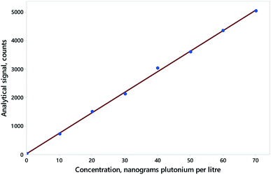Fig. 1 Calibration for ²³⁹Pu by ICP-MS, using responses from column “R1”, showing data (blue points) and simple regression (red line). Data (from AMC Datasets) can be found at http://www.rsc.org/images/Plutonium239_tcm18-57760.txt.

Fig. 2 illustrates the effect of the dependence on the outcome for the calibration shown in Fig. 1. Point A in Fig. 2 shows the values of the estimated coefficients. Points B and C show example reference pairs of values defining illustrative joint null hypotheses, that is,

H₀: α = α_ref and β = β_ref.

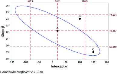Fig. 2 Outcome of regression on data from Fig. 1, showing the regression coefficients (Point A), their individual 95% confidence limits (outer dashed lines), the limit of the 95% joint confidence region (blue ellipse), and two example joint null hypotheses (points B, C).

Point B falls within both of the individual 95% confidence intervals, so the regression coefficients (Point A) might naively be taken as showing no significant difference from the reference values. Crucially, however, point B falls outside the ellipse defining the joint confidence region, and the joint null is therefore properly rejected at 95% confidence. Point C, in contrast, falls outside the two individual confidence intervals, so might be taken as significantly different and rejected on both counts. However, it is clearly within the joint 95% confidence region and therefore the null hypothesis is not rejected.

These examples serve as an illustration for interpreting joint confidence regions but, for calibration purposes, an analyst would usually be interested in testing only the single null hypothesis that the intercept was zero, α = 0. A zero intercept is useful as it means that the signal is proportion to the concentration. In any event, the slope of the graph is usually set at an arbitrary value. In Fig. 2 we see that zero is comfortably within the confidence limits (−82.5, 118.9) for the separate intercept estimate.

Comparison of two procedures for bias

In this section we consider the comparison between paired results from two analytical procedures applied to numerous different test materials. Translational bias would be present if α ≠ 0, rotational bias if β ≠ 1. At first sight it seems as though we should test the respective null hypotheses separately. However, because of the correlation between the coefficients we can validly test only the joint outcome for inferring bias (or its absence) between the analytical procedures. In such cases we can formulate a joint null hypothesis, namely,

H₀: (α = 0 and β = 1).

Random variation aside, that is what we would expect if there were no bias at all.

Fig. 3 shows some results from a comparison of a laboratory-based reference method and a field method for the determination of uranium in stream waters sampled at various sites, using unweighted regression. Fig. 4 shows the discrepant outcomes of both separate and joint tests of significance. In that instance the null hypothesis value for the slope coefficient β (that is, 1.0 exactly) is outside (just) the upper confidence limit for the slope estimate, and so might be naively taken as implying a significant rotational bias. The combined null point (0, 1), however, is clearly within the joint confidence region, so any bias indicated is not significant at 95% confidence.

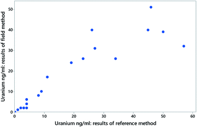Fig. 3 Data (blue solid circles) from a comparison between an experimental field method and a laboratory reference method for the determination of uranium in stream water (excluding values above 100 ng ml⁻¹). Each point is from a separate source of water. Here the laboratory method is assumed to have the smaller variance and is treated as the independent variable. Data (from AMC Datasets) can be found at http://www.rsc.org/images/Uranium_in_stream%20water_tcm18-57750.txt.

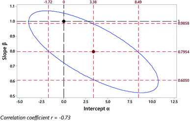Fig. 4 Outcome of regression on data from Fig. 3, showing the regression coefficients (central point), their individual 95% confidence limits (outer red dashed lines), the limit of the joint 95% confidence region (blue ellipse), and a joint null hypothesis H₀: (α = 0 and β = 1) (black dashed lines and point).

The data shown in Fig. 5, a comparison of a rapid procedure and a reference procedure for the determination of dissolved oxygen in samples of water, gives rise to a contrasting outcome. The correlation between the coefficients is more extreme than in the previous example, and the joint confidence region correspondingly narrow (Fig. 6). There we see the combined null point (0, 1) well within both of the individual 95% confidence limits, suggesting prima facie that there is no bias in the rapid procedure. However, the null point is clearly outside the joint 95% confidence region, showing that significant bias is indeed present, although not showing exactly what form the bias takes.

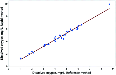Fig. 5 Data (blue solid circles) and simple regression (red line) from a comparison between an experimentally rapid method and a laboratory reference method for the determination of dissolved oxygen in water. Each point is from a separate source of water. Here the laboratory method is assumed to have the smaller variance and is treated as the independent variable. The value at about 9 mg L⁻¹ was excluded from further treatment as it seems to be an outlier and leverage point. Data (from AMC Datasets) can be found at http://www.rsc.org/images/Dissolved%20oxygen_tcm18-194855.txt.

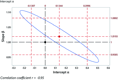Fig. 6 Outcome of regression on data from Fig. 5 (excluding high leverage point), showing the regression coefficients (central point), their individual 95% confidence limits (outer red dashed lines), the limit of the joint 95% confidence region (blue ellipse), and the joint null hypothesis H₀: (α = 0 and β = 1) (black dashed lines and point).

It should be noted that in each of these comparisons it is assumed that the reference method (i.e., the independent variable) has a much smaller variance than the other method. If a reference procedure used in method comparison has an appreciable variance, it may be preferable to use the FREML (functional relationship estimation by maximum likelihood) approach, as described in Technical Brief 10: an Excel® add-in for this method is available via the RSC web site. The datasets used in this Technical Brief can also be downloaded without formality via the Analytical Methods Committee webpages at http://www.rsc.org/amc.

Calculations

The method for calculating joint confidence regions is simple in principle when applied to ordinary (i.e., unweighted) least squares regression but requires attention to detail in practice. With predictor variable x₁… x_n, the formula defining the dependence between potential values of zero-centred coefficients [small alpha, Greek, tilde] and [small beta, Greek, tilde] is

[small beta, Greek, tilde]²Σx² + [small beta, Greek, tilde](2[small alpha, Greek, tilde]Σx) + n[small alpha, Greek, tilde]2 − 2s²F = 0,

where F represents the one-tailed variance ratio statistic F_2,n−2 for the required level of confidence and s², the mean square error. This is a quadratic equation in [small beta, Greek, tilde] with roots

By inserting any appropriate value of [small alpha, Greek, tilde], we obtain two real values of [small beta, Greek, tilde], which define points on opposite sides of the confidence ellipse. At the poles of the ellipse the two roots are equal, outside that range there are no real roots. The points obtained are re-centred on the regression coefficients and plotted by joining adjacent points. A version for weighted regression is a straightforward extension of this procedure.

Conclusion

The negative correlation between the estimates of the slope and the intercept of a regression line is clearly an important and often-neglected issue in the interpretation of calibration and method comparison plots: failure to appreciate its significance could lead to entirely incorrect interpretations of such procedures.

Further reading

Massart et al., 1997 D. L. Massart et al., Handbook of Chemometrics and Qualimetrics, Part A (1997), Elsevier, Amsterdam, Chapter 8.

M. Thompson (Birkbeck University of London).

This Technical Brief was written on behalf of the Statistics Expert Working Group and approved by the Analytical Methods Committee on 28/02/19.

---