
 Open Access Article
 This Open Access Article is licensed under a
 Creative Commons Attribution 3.0 Unported Licence
Emerging patterns in the global distribution of dissolved organic matter fluorescence†
Urban J.
Wünsch
 *a,
Rasmus
Bro
b,
Colin A.
Stedmon
c,
Philip
Wenig
d and
Kathleen R.
Murphy
a
*a,
Rasmus
Bro
b,
Colin A.
Stedmon
c,
Philip
Wenig
d and
Kathleen R.
Murphy
a
aChalmers University of Technology, Architecture and Civil Engineering, Water Environment Technology, Sven Hultins Gata 6, 41296 Gothenburg, Sweden. E-mail: wuensch@chalmers.se
bUniversity of Copenhagen, Dept. Food Science, 1958 Frederiksberg, Denmark
cNational Institute of Aquatic Resources, Technical University of Denmark, Kemitorvet, 2800 Kgs. Lyngby, Denmark
dLablicate GmbH, Martin-Luther-King Platz 6, 20146 Hamburg, Germany
First published on 17th January 2019
Abstract
The spectra responsible for natural dissolved organic matter (DOM) fluorescence in 90 peer-reviewed studies have been compared using new similarity metrics. Numerous spectra cluster in specific wavelength regions. The emerging patterns suggest that most fluorescence spectra are not tied to biogeochemical origin, but exist across a wide range of different environments.
Introduction
Fluorescence spectroscopy can characterize chromophores in dilute mixtures in the ultraviolet-visible (UV-vis) wavelength range,1 and is a popular tool for the untargeted analysis of chemically complex samples such as solutions containing dissolved organic matter (DOM).2,3The analysis of fluorescence emission excitation matrices (EEMs) most often assumes that observed fluorescence is due to the superposition of several distinct but overlapping fluorescence spectra. Thus, EEMs show broad emission spectra whose emission maxima increase towards longer excitation wavelengths (Fig. 1). Such mixtures can be described by “picking” the fluorescence intensities at predefined wavelength pairs that have been assigned names such as “peak C”, “peak A”, or “peak T” (Fig. 1, black letters).4 Alternatively, the fluorescence intensities in wavelength regions of an EEM can be summed up, as in the fluorescence regional integration (FRI) approach (Fig. 1, white letters).5 However, such approaches may sum up the fluorescence of multiple fluorophores.
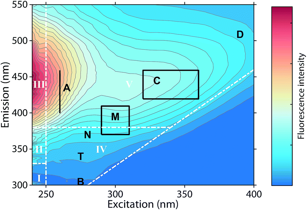 | ||
| Fig. 1 Typical emission excitation matrix (EEM) of dissolved organic matter (Öre estuary, Sweden). White inserts refer to the five regions defined through fluorescence regional integration (FRI).5 Black inserts refer to wavelengths pairs at which fluorescence intensities are “picked”.4 | ||
In contrast, trilinear models such as parallel factor analysis (PARAFAC) decompose EEMs into underlying statistical components, producing a set of corresponding excitation and emission spectra that, when multiplied by the correct weights (scores) and summed, can reproduce every EEM in the original dataset. Because fluorescence properties of chromophores are generally tied to molecular structures and respond to changes on the molecular level, PARAFAC components may also reveal information about the chemical structures responsible for their properties.6 However, the chemical origin of DOM fluorescence and the true number of distinguishable phenomena remains unknown. Thus, despite the high similarity of EEMs across environments, individual PARAFAC models are developed for new datasets with no assumptions made about the presence of particular spectra.7,8
To aid the interpretation of PARAFAC components and identify the potential emergence of global patterns, a community-driven database called OpenFluor was established in 2014.9 As of the publication of this article, OpenFluor contains over 100 entries and more than 500 PARAFAC component spectra mainly describing DOM fluorescence in natural and engineered systems (Fig. 2). Although OpenFluor is widely used to evaluate similarities between pairs of spectra, systematic trends of PARAFAC spectra in the database have not been reported.
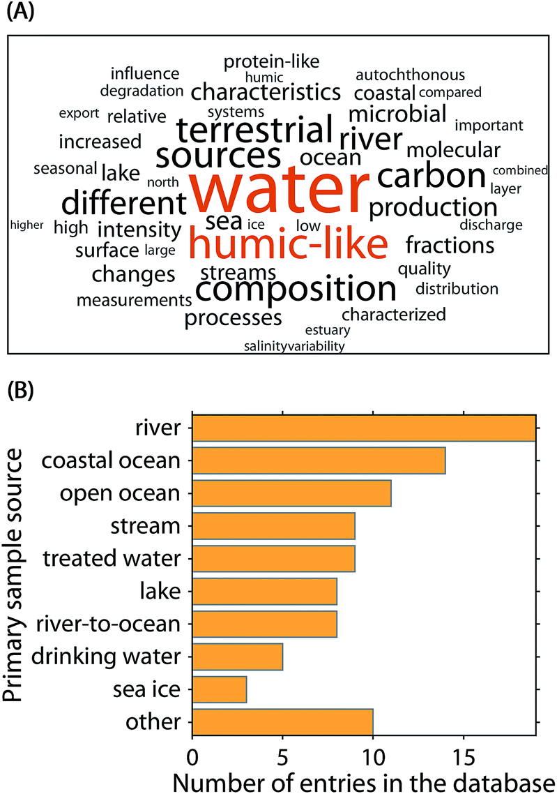 | ||
| Fig. 2 Meta-analysis of the 90 OpenFluor database entries analysed in this study. (A) Fifty most frequent words in the publication abstracts. (B) Most frequently reported sample origins. | ||
In order to identify similar fluorescence component spectra, sensitive metrics of similarity are required. For DOM fluorescence, the Tucker congruence coefficient (TCC) has been adopted.10 However, experience shows that the TCC does not adequately address the generally high resemblance of spectra, particularly if they are Gaussian-shaped. The reliable identification of patterns in large databases requires more sensitive algorithms.
Here, we develop a new metric called shift- and shape sensitive congruence (SSC) and use it to identify patterns in the global occurrence of DOM fluorescence spectra according to data in OpenFluor. SSC is based on Tucker's congruence but is more sensitive to subtle differences in peak positions and peak broadness. Additionally, we establish a new approach to quantify similarity between fluorescence models.
Experimental section
OpenFluor
Ninety published fluorescence datasets were extracted from the OpenFluor database (http://www.openfluor.org). Each dataset represented a single PARAFAC decomposition (model) of an independently sampled dataset and its associated metadata. Models contained a set of three to eight excitation and emission spectra that together represent all the underlying fluorescence components that varied independently in that study. All spectra (N = 478) were interpolated to identical wavelength increments and ranges (270–440 nm excitation, 300–540 nm emission), smoothed, and normalized by their Frobenius norm. Positions of the primary emission peak and first excitation peak (when plotted against wavenumber) were used to calculate the Stokes shift.11 Full details on the processing of spectra can be found in the ESI (section S1†).Assessment of component congruence
To sensitively assess the similarity between PARAFAC spectra, we developed the shift- and shape sensitive congruence coefficient as a modification of the Tucker congruence coefficient.10,12 The SSC penalizes mismatches in fluorescence peak area and maxima in comparisons between two spectra follows:| SSC(x,y) = TCC − (α + β) | (1) |
The two penalty terms α and β accounted for differences between two spectra x and y with regards to shape (β) and peak wavelength position (α). Further details on the calculation of α and β and their sensitivity to differences between spectral shapes are shown in Fig. 3 and given in the ESI (section S2†).
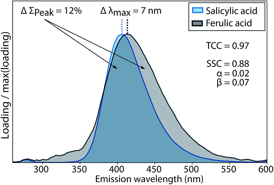 | ||
| Fig. 3 Evaluation of fluorescence emission spectrum similarity of salicylic and ferulic acid by TCC and SSC. ΔΣPeak refers to the difference in the peak integrals and Δλmax refers to the difference in peak wavelength. The two penalty terms α, β quantify differences in peak position and peak area between both spectra. | ||
The SSC was developed primarily to address a lack of sensitivity in TCC that is evident when comparing emission spectra, since these are unimodal and superficially more similar than multipeak excitation spectra. For example, emission peaks that differ by more than 15 nm in peak wavelength often have high Tucker congruence. Thus, we used the SSC for comparing emission spectra while excitation spectra were compared using the previously established TCC.
Assessment of model similarity
Each model in OpenFluor contains the excitation and emission spectra of several underlying fluorescence components reported to vary in relative concentration in a published study. An objective of the current study was to determine the similarity between collections of fluorescence components (i.e. between models). Here, we assessed the question of model similarity by focusing on the degree of spectral similarity between the components in different models. The following system was devised for comparing models with different numbers of fluorescence components: if a model X with n components was compared to another model Y with n + m components, then the best n comparisons were considered while the worst m comparisons were omitted: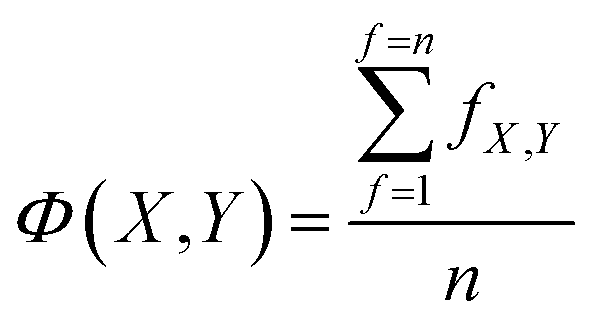 | (2) |
Results and discussion
Assessment of spectral similarity
The conventional Tucker congruence coefficient was less sensitive than the newly developed shift- and shape sensitive congruence (ESI section S2†). SSC uses the conventional TCC to assess overall shape similarity, but additionally quantifies differences in emission peak position (term α in eqn (1)) and peak areas (term β in eqn (1)). Fig. 3 shows how the conventional TCC and its general interpretation (good match > 0.95)10,12 would lead to the conclusion that the fluorescence emission spectra of salicylic and ferulic acid are interchangeable, while the corresponding SSC is far lower due to differences in peak integral and peak wavelength position. SSC is thus a sensitive metric to assess the similarity of fluorescence emission spectra with generally high resemblance.For TCC, 0.95 has been proposed as a threshold value for good similarity, whereas achieving the same score of SSC would require a better match between two spectra. In scenarios where the high quality of spectral matches is central to an interpretation, SSC would provide a more stringent assessment compared to TCC. One such scenario is model validation, where two models derived on independent halves of an overall data set are compared. Another scenario is the comparison of PARAFAC spectra between studies or with spectra of pure substances, where claims of identity have a significant impact on the (biogeochemical) interpretation of components. Reporting high scores for SSC rather than TCC would provide superior support for interpretations in these cases.
Spectral patterns in DOM fluorescence
The 478 PARAFAC component spectra in OpenFluor showed a wide range of excitation and emission peak positions and Stokes shifts (Fig. 4). Excitation peaks ranged from 270 to 427 nm with a median of 308 nm. Fluorescence emission peaks spanned the entire range of measured emission wavelengths (300–540 nm), whereby half of the components described fluorescence emission in the ultraviolet range (<416 nm). Components had an average Stokes shift of 0.85 ± 0.31 eV. In comparison, simple fluorophores have Stokes shifts in the range of 0.3–1.4 eV.13 94% of all components in OpenFluor had a Stokes shift in this range (Fig. 4). This demonstrates that, while the description of DOM fluorescence by PARAFAC makes no assumptions regarding peak shapes or positions, the resulting statistical components largely have viable Stokes shifts.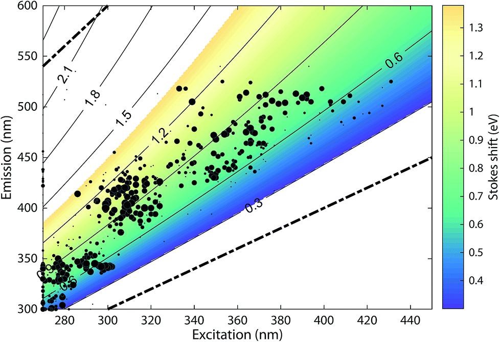 | ||
| Fig. 4 Peak location of 478 PARAFAC components and their Stokes shift. Contour lines show Stokes shifts in the wavelength range of the depicted EEM, while the coloured region depict the typical range observed for pure compounds (0.3–1.4 eV). All dots are sized according to the frequency with which they match other components in the database (also see Fig. 5). The two dashed lines represent the location of Rayleigh scatter. | ||
Numerous published fluorescence components fell within the fluorescence emission range of the classic DOM peaks defined in previous works (Table 1, Fig. 5).4,14 In 66.7% of studies, a component falling within the range of peak C was identified. Components exhibiting fluorescence in the ranges of peaks B, T, M, A, and D were less frequently identified (45.5, 40, 36.6, 16.7, and 8.9% of studies respectively, Table 1). These results indicate that some of the peaks identified historically through raw data analysis are also frequently identified as components in PARAFAC. This is particularly the case in the centre of the EEM (peak C), where fluorescence signals are high, spectral corrections are reliable, and instruments perform well. However, PARAFAC often identified components outside of, or in between the classic peak ranges.
| Peak | λ Ex/λEm | % OpenFluor studies |
|---|---|---|
| A | 260/400–460 (+20 nm) | 16.7 |
| B | 275/305 (±10) | 45.5 |
| T | 275/340 (±10) | 40 |
| M | 370–410/290–310 | 36.6 |
| C | 320–360/420–460 | 66.7 |
| D | 390/509 (±10) | 8.9 |
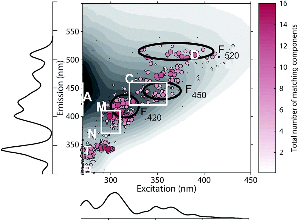 | ||
| Fig. 5 Excitation and emission maxima of 478 DOM fluorescence components. Dots are coloured and sized according to the frequency with which they match other database components. The background contour plot shows a typical riverine EEM for reference (Columbia River, USA). Match-weighted probability density plots show the distribution of emission and excitation peaks along the corresponding axis. For reference, traditional peaks are plotted (white) along with the ranges of recently defined ubiquitous components F520, F450, and F420 (black Murphy et al., [2018]). | ||
On average, each component in OpenFluor showed high spectral congruence (TCCEx > 0.95, SSCEm > 0.95) with 3.8 ± 3.6 other components in the database. This increased to 4.9 ± 3.4 if components with no matches were excluded (N = 111). The most frequently matching components showed high similarity with up to 16 other entries (Fig. 5). When components were plotted according to their excitation and emission peaks and weighted by their match-frequency in the database (Fig. 4 and 5), six distinct clusters could be identified: (1) components similar to classic peak T (λEx/λEm 275/340); (2) components similar to peak T, but with excitation maxima closer to 300 nm; (3) components located between peak M and C (λEx/λEm 300–330/380–430); (4) components similar to peak C (λEx/λEm 330–360/420–455); (5) components similar to group 4, but with longer emission maxima near 480 nm; (6) components similar to peak D with emission maxima between 500 and 520 nm and a wide range of excitation maxima.
The clustering of peaks in groups 1, 2, and 4 largely agrees with known peak locations reported earlier by Coble (2007) and provides independent evidence for the frequent occurrence of fluorescence peaks in these regions. However, group 3 notably diverges from these predefined peaks, since this group was located between peaks M and C. The frequent identification of peaks in this region by PARAFAC and a lack of identification by peak-picking is most likely a consequence of the highly overlapping nature of fluorescence components in this wavelength region. Similarly, the clustering of PARAFAC spectra between 450 and 490 nm (group 5) also does not agree with predefined “picked” peaks, or the peak positions of recently proposed ubiquitous PARAFAC spectra emitting at 417 ± 10 nm (F420), 445 ± 6 nm (F450), or 514 ± 9 nm (F520).15
Since PARAFAC modelling depends on choosing an appropriate number of components, it is susceptible to fitting models with too few or too many components. While protection against overfitting is usually provided through validation methods, the identification of underspecified models is more difficult. Such models are typically chosen as a compromise due to small sample sizes, low overall signal intensity, or highly correlated abundances of the underlying spectra.8 The use of too few components results in the description of fluorescence properties of multiple components in one “averaged” component (as demonstrated in ESI section S3†). The occurrence of components in group 5 (emission peaks near 480 nm) may be related to underspecified models having fewer than three components emitting in the visible wavelength range. Of the 90 analysed models, 53% featured two or less components with emission maxima > 420 nm, while a recent study suggests that the adequate description of DOM fluorescence requires at least three components emitting in the visible range.15
The challenge of fitting the appropriate number of components to model DOM fluorescence is especially critical in datasets with small sample sizes or little spectral variability. Recent studies demonstrate that such challenges can be addressed with methods that selectively influence the underlying constituents of fluorescent DOM in a single sample (through e.g. photochemistry or chromatography) in a manner that allows robust statistical descriptions (“one-sample PARAFAC”).15,16 Future studies can benefit from such methods and we hypothesize that this will result in a convergence towards more similar fluorescence components across independent studies.15
Similarity between PARAFAC models
The average similarity between PARAFAC models ranged from 0.37 to 0.97 (mean 0.84) for ΦEm, and 0.45 to 0.99 (median 0.89) for ΦEx. Twenty-four models in the database were highly similar to at least one other model (ΦEm and ΦEx > 0.95). While this only represents a small fraction of comparisons (0.3% of 90 × 89 comparisons between 90 models), a high model similarity may not be expected in comparisons involving multiple components since average model similarity scores are significantly impacted by the presence of any mismatching component. Artefacts possibly introduced due to laboratory-, instrument-, user-, and environment-specific factors may serve to further increase differences between models.17,18Fig. 6 shows an example comparison of a six-component model of DOM fluorescence in the Otonabee River.19 In this case, the most-similar amongst the 89 remaining models was found to be a five-component model of DOM fluorescence in boreal lakes and rivers where three components matched well between both studies.20,21 The average congruence of the five most similar components was 0.96 (ΦEm) and 0.95 (ΦEx) and the two models generally show good agreement. Our approach to investigating model similarity may be useful to quickly identify highly congruent models in spectral databases such as OpenFluor.
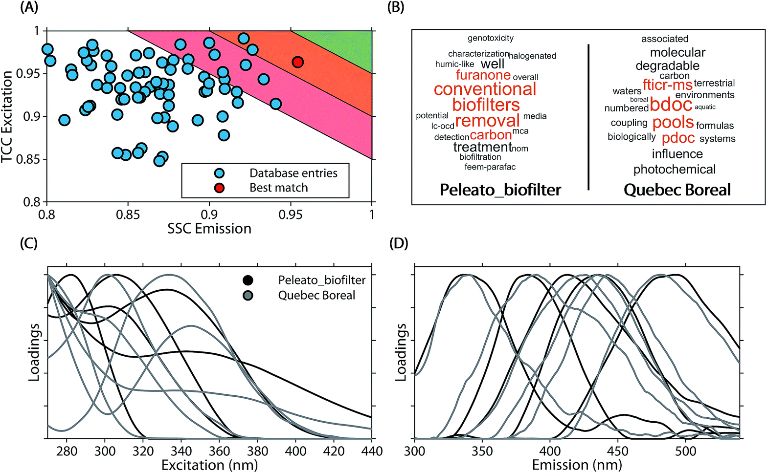 | ||
| Fig. 6 Comparison of a five component PARAFAC model (Peleato_biofilter19) with other models in the OpenFluor database. (A) Average emission SSC (ΦEm) and excitation TCC (ΦEx) between the five components in Peleato_biofilter and components in all models of the OpenFluor database. Green, orange and red patches encompass average high (>0.95), medium (>0.9<0.95), and low (>0.85<0.9) similarity. (B) Word clouds of abstracts belonging to the reference model and the best-matching database entry (Quebec Boreal20,21). (C, D) Excitation and emission spectra of Peleato_biofilter (black) and Quebec Boreal (grey). | ||
Many studies in recent years have sought to use fluorescent components of DOM to discriminate between chemical fractions and biogeochemical sources of DOM. Often, the specificity of components as proxies for terrestrial or microbial fractions is inferred. If this assumption held true, fluorescence models describing DOM in different biogeochemical contexts may also be distinguishable. However, since DOM is often highly conserved,22 and its chemical character is similar across many environments,23 a lack of specificity that reflects the ubiquitous processes governing the turnover of organic molecules in aquatic environments may be expected. Our meta-analysis of the 90 fluorescence models indeed suggests this lack of specificity (ESI section S4†). Patterns of model similarity were not driven by DOM biogeochemistry. Instead, there was a tendency for models with similar number of components to be good matches, particularly the number of components with visible wavelength fluorescence featuring emission maxima > 400 nm (Fig. 7). This indicates that the results of inter-study comparisons are likely dependent on the number of components chosen to describe a particular dataset, i.e. studies describing DOM fluorescence with similar number of components tend to converge towards similar solutions. Moreover, our analysis indicated that methodological similarities (e.g. particular choices made by users involving wavelength ranges, increments, instruments, integration time) may contribute towards model similarity (Fig. S5†). Further developments in the application of PARAFAC to DOM fluorescence should therefore focus on estimating the impact of instrument settings and other parameters on the modelling outcome to improve the comparability of globally acquired datasets.
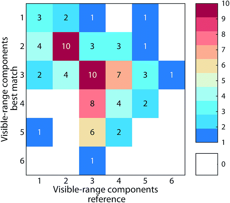 | ||
| Fig. 7 Frequency of models best matching database entries with equal or different number of components in the visible wavelength range (emission maxima > 400 nm). Matches along a diagonal line of equal numbers indicate a relationship between model similarity and number of humic-like components. | ||
Conclusions
The newly developed shape- and shift-sensitive congruence presents a sensitive metric to assess subtle differences between fluorescence emission spectra of fluorescent DOM and, in combination with the comparison of corresponding excitation spectra, reduces the risk of falsely identifying significant spectral similarity. The SSC may in the future be useful in studies seeking to identify highly similar components of fluorescent DOM or establish links between DOM fluorescence and pure organic substance fluorescence.An analysis of 90 peer-reviewed PARAFAC models revealed that most PARAFAC fluorescence spectra of DOM exhibit properties typical for fluorophores. In the past, a central hypothesis has been that these independent spectra represent different biogeochemical fractions of DOM.1 In contrast to this hypothesis, we identified six key regions of fluorescent DOM components across numerous geographical regions. A meta analyses revealed no clear connection between fluorescence spectral composition and DOM biogeochemistry. These findings provide evidence that certain fluorescence components reoccur irrespective of sample source. While methodological biases may contribute to this result, another possible interpretation is that physicochemical reactions act upon DOM to produce a set of highly conserved fluorescence spectra.15 Further investigation of this hypothesis is warranted, and methodological developments are required to utilize information about reoccurring fluorescence species in DOM.
The attribution of DOM fluorescence to specific chemical compounds remains largely unachieved.13 Therefore, deeper insights into the biogeochemistry of DOM fractions require linking fluorescence to complementary chemical information. Studies in recent years have demonstrated the benefits of DOM multidetector analysis to the interpretation of fluorescence.24–26 This approach combines the strengths of individual detection methods and thus may provide further advances in the characterization of DOM.
Conflicts of interest
There are no conflicts to declare.Acknowledgements
The authors acknowledge all scientists that have contributed to this study by sharing their data via the OpenFluor database. Significant advances in the understanding of DOM fluorescence rely on such community-driven efforts. The authors acknowledge funding from the Swedish Research Council (FORMAS 2017-00743).Notes and references
- P. G. Coble, Mar. Chem., 1996, 51, 325–346 CrossRef CAS.
- J. B. Fellman, E. Hood and R. G. M. Spencer, Limnol. Oceanogr., 2010, 55, 2452–2462 CrossRef CAS.
- K. R. Murphy, A. Hambly, S. Singh, R. K. Henderson, A. Baker, R. M. Stuetz and S. J. Khan, Environ. Sci. Technol., 2011, 45, 2909–2916 CrossRef CAS PubMed.
- P. G. Coble, Chem. Rev., 2007, 107, 402–418 CrossRef CAS PubMed.
- W. Chen, P. Westerhoff, J. A. Leenheer and K. Booksh, Environ. Sci. Technol., 2003, 37, 5701–5710 CrossRef CAS PubMed.
- J. R. Lakowicz, Principles of fluorescence spectroscopy, New York, 3rd edn, 2006 Search PubMed.
- C. A. Stedmon, S. Markager and R. Bro, Mar. Chem., 2003, 82, 239–254 CrossRef CAS.
- K. R. Murphy, C. A. Stedmon, D. Graeber and R. Bro, Anal. Methods, 2013, 5, 6557–6566 RSC.
- K. R. Murphy, C. A. Stedmon, P. Wenig and R. Bro, Anal. Methods, 2014, 6, 658–661 RSC.
- U. Lorenzo-Seva and J. M. F. ten Berge, Methodology, 2006, 2, 57–64 CrossRef.
- D. M. Reynolds, in Aquatic Organic Matter Fluorescence, ed. P. Coble, J. Lead, A. Baker, D. M. Reynolds and R. G. M. Spencer, Cambridge University Press, Cambridge, 2014, pp. 3–34 Search PubMed.
- L. R. Tucker, in Personnel Research Section Report No. 984, Department of the Army, Washington D.C., 1951 Search PubMed.
- U. J. Wünsch, K. R. Murphy and C. A. Stedmon, Frontiers in Marine Science, 2015, 2, 1–15 CrossRef.
- C. H. Lochmüller and S. S. Saavedra, Anal. Chem., 1986, 58, 1978–1981 CrossRef.
- K. R. Murphy, S. A. Timko, M. Gonsior, L. C. Powers, U. J. Wünsch and C. A. Stedmon, Environ. Sci. Technol., 2018, 52, 11243–11250 CrossRef CAS PubMed.
- U. J. Wünsch, K. R. Murphy and C. A. Stedmon, Environ. Sci. Technol., 2017, 51, 11900–11908 CrossRef PubMed.
- K. R. Murphy, K. D. Butler, R. G. M. Spencer, C. A. Stedmon, J. R. Boehme and G. R. Aiken, Environ. Sci. Technol., 2010, 44, 9405–9412 CrossRef CAS PubMed.
- C. L. Osburn, R. Del Vecchio and T. J. Boyd, in Aquatic Organic Matter Fluorescence, ed. P. Coble, J. Lead, A. Baker, D. M. Reynolds and R. G. M. Spencer, Cambridge University Press, Cambridge, 2014, pp. 233–277 Search PubMed.
- N. M. Peleato, M. McKie, L. Taylor-Edmonds, S. A. Andrews, R. L. Legge and R. C. Andrews, Chemosphere, 2016, 153, 155–161 CrossRef CAS PubMed.
- A. Stubbins, J.-F. Lapierre, M. Berggren, Y. T. Prairie, T. Dittmar and P. A. del Giorgio, Environ. Sci. Technol., 2014, 48, 10598–10606 CrossRef CAS PubMed.
- J.-F. Lapierre and P. A. del Giorgio, Biogeosciences, 2014, 11, 5969–5985 CrossRef.
- R. Flerus, O. J. Lechtenfeld, B. P. Koch, S. L. McCallister, P. Schmitt-Kopplin, R. Benner, K. Kaiser and G. Kattner, Biogeosciences, 2012, 9, 1935–1955 CrossRef CAS.
- M. Zark and T. Dittmar, Nat. Commun., 2018, 9, 3178 CrossRef PubMed.
- C. Romera-Castillo, M. Chen, Y. Yamashita and R. Jaffé, Water Res., 2014, 55, 40–51 CrossRef CAS PubMed.
- C. W. Cuss and C. Guéguen, Water Res., 2015, 68, 487–497 CrossRef CAS PubMed.
- U. Wünsch, E. Acar, B. P. Koch, K. R. Murphy, P. Schmitt-Kopplin and C. A. Stedmon, Anal. Chem., 2018, 90, 14188–14197 CrossRef PubMed.
Footnote |
| † Electronic supplementary information (ESI) available: Definitions of shift- and shape sensitive congruence , information on the processing of OpenFluor models, and meta-analysis of model similarities. See DOI: 10.1039/c8ay02422g |
| This journal is © The Royal Society of Chemistry 2019 |