
Deep learning-based component identification for the Raman spectra of mixtures†
Xiaqiong
Fan
,
Wen
Ming
,
Huitao
Zeng
,
Zhimin
Zhang
 * and
Hongmei
Lu
*
* and
Hongmei
Lu
*
College of Chemistry and Chemical Engineering, Central South University, Changsha, China. E-mail: zmzhang@csu.edu.cn; hongmeilu@csu.edu.cn
First published on 23rd January 2019
Abstract
Raman spectroscopy is widely used as a fingerprint technique for molecular identification. However, Raman spectra contain molecular information from multiple components and interferences from noise and instrumentation. Thus, component identification using Raman spectra is still challenging, especially for mixtures. In this study, a novel approach entitled deep learning-based component identification (DeepCID) was proposed to solve this problem. Convolution neural network (CNN) models were established to predict the presence of components in mixtures. Comparative studies showed that DeepCID could learn spectral features and identify components in both simulated and real Raman spectral datasets of mixtures with higher accuracy and significantly lower false positive rates. In addition, DeepCID showed better sensitivity when compared with the logistic regression (LR) with L1-regularization, k-nearest neighbor (kNN), random forest (RF) and back propagation artificial neural network (BP-ANN) models for ternary mixture spectral datasets. In conclusion, DeepCID is a promising method for solving the component identification problem in the Raman spectra of mixtures.
1. Introduction
Raman spectroscopy can retrieve vibrational information from molecules and is often used as a fingerprint technique to identify components in samples. It has the advantages of being fast and non-invasive and allows pre-treatment-free analysis in the field.1,2 However, it is still challenging to elucidate the hidden molecular structural information in Raman spectra,3–5 especially in the spectra of mixtures. Therefore, various chemometric methods have been developed to identify the components in Raman spectra.Searching algorithms combined with databases is the most important method to solve the problems of component identification. The construction of databases can provide researchers with a powerful tool to elucidate Raman spectra.6 In fact, Raman databases are the core of many applications. Nowadays, many researchers have established relevant databases, such as database for the Raman spectra of 21 azo pigments,7 database of FT-Raman spectra,8 e-VISART database,9 biological molecule database,10 explosive compound database,11 and pharmaceutical raw material database,12 for the rapid and non-destructive identification of samples. With the increasing number of databases, various searching algorithms13–16 have been developed. Most of them measure the similarity between Raman spectra using correlation, Euclidean distance, absolute value correlation and least-squares.17 However, these correlation- and distance-based methods are effective only for the comparison of pure components. In practical application, multi-components are usually present in the Raman spectra of complex samples. Therefore, there is an urgent need to develop algorithms to identify the components in the Raman spectra of mixtures.
For component identification with Raman spectra of mixtures, many statistics and chemometric methods have been proposed. The reverse search18 compares a subset of peaks in an unknown spectrum with the spectra in the database, which is more effective than the forward search method for component identification in mixtures. The interactive self-modelling method (SIMPLISMA)19 was developed by Winding to extract a pure spectrum from a mixture according to the purity spectrum and standard deviation spectrum. A spectral reconstruction algorithm20 based on minimum information entropy has been developed to recover the individual spectrum contained in mixtures without any database or priori knowledge when there is a significant number of mixture spectra. An automatic system has been presented to identify the Raman spectra of binary mixtures of pigments, with good robustness against some of the critical factors.21 A component identification method22 has been established based on the partial correlation of each component identified. The generalized linear model has been used to compute the probability that an identified component is truly present in a mixture. Recently, the sparse regularized model23 has been proposed as a complement to traditional regression methods to decompose the Raman spectra of a mixture and identify the target components. The reverse searching and non-negative least square (RSearch-NNLS)12 method has demonstrated outstanding performances for component identification and ratio estimation; however, it requires lots of spectral pre-processing including smoothing, baseline correction and peak detection.
Most of the abovementioned methods are based on the similarity or distance between spectra, the characteristic peaks and the database searching algorithms. The choice of searching algorithm, similarity criteria and characteristic peaks will significantly affect the identification results. Furthermore, spectral pre-processing, an essential step in these methods, has the potential risk to introduce errors and variability.24,25 Therefore, these factors may have an impact on the accuracy of the component identification of mixtures.
Deep learning is one of the most focused research fields in recent years, aiming to learn features and directly build predictive models from large-scale raw datasets.26 It shows excellent performances in many fields of chemistry and biology including spectroscopy,27–31 proteomics,32–34 metabolomics35,36 and genomics.37,38 These applications demonstrate the advantages of deep-learning techniques in signal-extraction, feature-learning and modelling complex relationships. Convolutional neural network (CNN) is an important branch of deep learning technology. It is inspired by the biological visual cognition mechanism.39 The neural network model Neocognitron40 for visual pattern recognition, proposed by Kunihiko Fukushima, is considered to be the predecessor of CNN. Other representative neural networks, such as wavelet neural network (WNN),41 have also been developed according to the visual characteristics of multi-resolution, local correspondence and direction. In the 1990s, the framework of modern CNN was determined by Lecun et al.,42,43 called LeNet-5. In terms of image representation and digital recognition, LeNet-5 exhibits great performances; however, it is not suitable for complex problems due to the lack of data and limited computing capabilities. In recent years, various methods have been developed for the effective training of deep CNN. The deeper CNN AlexNet44 has achieved excellent performances with the rectified linear unit (ReLU)45 and dropout46 methods. Other methods such as ZFNet,47 VGGNet,48 GoogleNet49 and ResNet50 are all representative CNNs.
In this study, deep learning-based methods were used to directly identify the components in mixtures from raw Raman spectra. CNN models were built for each compound in the database to achieve the aim of component identification in mixtures. The proposed deep learning-based component identification (DeepCID) can distil useful information from raw Raman spectra and identify the components of mixtures.
2. Method
In this study, data augmentation was applied for each compound in the database. Then, one-component identification (identification of a specific component) models were built using CNN to predict the existence of each compound in the mixtures. All the one-component identification models were trained and stored in a hard disk for reload. The simulated datasets, liquid and powder mixture dataset and ternary mixture dataset were used to test the performance of DeepCID. The flowchart of DeepCID and the architecture of CNN are shown in Fig. 1.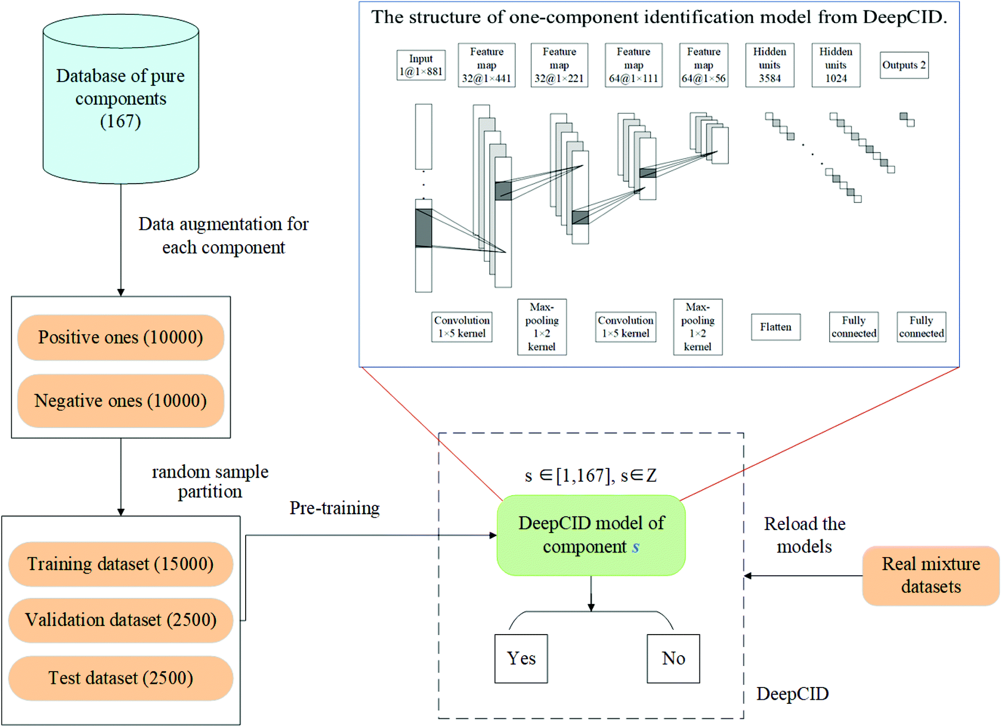 | ||
| Fig. 1 Flowchart for DeepCID and the architecture of the CNN model. The spectrum of each pure compound in the database is used for data augmentation, and both positive and negative samples are generated with equal size. The augmented dataset of each compound is divided into three parts for training, validation and testing. The 167 one-component identification models are trained and saved for further prediction. The architecture of the CNN model is shown in the top right corner. A four-layer CNN model is used in DeepCID. The first two layers are convolutional layers, and the last two layers are fully connected layers. The number of convolution output dimensions is 32 and 64, and the number of nodes in the fully connected layers is 1024 and 2. DeepCID can be easily and quickly reloaded for the prediction of components. | ||
2.1 Raman dataset
| No. | Status | Ratio | Components | Prediction results | TP | TN | FP | FN | TPR (%) | FPR (%) |
|---|---|---|---|---|---|---|---|---|---|---|
| 1 | Liquid | 5![[thin space (1/6-em)]](https://www.rsc.org/images/entities/char_2009.gif) :3:2 :3:2 |
Methanol | Methanol | 3 | 164 | 0 | 0 | 100.0 | 0.0 |
| Ethanol | Ethanol | |||||||||
| Acetonitrile | Acetonitrile | |||||||||
| 2 | Liquid | 7:2:1 |
Methanol | Methanol | 3 | 164 | 0 | 0 | 100.0 | 0.0 |
| Ethanol | Ethanol | |||||||||
| Acetonitrile | Acetonitrile | |||||||||
| 3 | Liquid | 4:3:3 |
Methanol | Methanol | 3 | 164 | 0 | 0 | 100.0 | 0.0 |
| Ethanol | Ethanol | |||||||||
| Acetonitrile | Acetonitrile | |||||||||
| 4 | Powder | 1:1 |
Polyacrylamide | Polyacrylamide | 2 | 165 | 0 | 0 | 100.0 | 0.0 |
| Sodium acetate | Sodium acetate | |||||||||
| 5 | Powder | 1:1:1 |
Polyacrylamide | Polyacrylamide | 3 | 164 | 0 | 0 | 100.0 | 0.0 |
| Sodium acetate | Sodium acetate | |||||||||
| Sodium carbonate | Sodium carbonate | |||||||||
| 6 | Powder | 5:3:2 |
Polyacrylamide | Polyacrylamide | 3 | 164 | 0 | 0 | 100.0 | 0.0 |
| Sodium acetate | Sodium acetate | |||||||||
| Sodium carbonate | Sodium carbonate | |||||||||
2.2 Data augmentation for each compound in the database
Data augmentation was applied to solve the problem of the limited number of Raman spectra during training, validation and testing. For each compound in the database, 20000 simulated mixture spectra were generated for both training and validation of its CNN model. The numbers of positive spectra (containing this compound) and negative spectra (not containing this compound) were both 10000. For the positive spectra, the ratios of the compound were randomly generated in [0.1, 1.0], and the ratios of the other interference compounds were randomly generated in [0.0, 1.0]. The negative spectra were generated by the superposition of the other compounds at random ratios in the [0.0, 1.0] range.
2.3 Spectra standardization and sample partition
The augmented dataset of each compound was divided into three parts: 15000 as the training set, 2500 as the validation set, and 2500 as the test set. The dataset of each compound was normalized to zero mean and unit variance at each Raman shift.
2.4 Convolutional neural network for component identification
CNN is a biologically inspired neural network, which consists of convolutional and subsampling layers optionally followed by fully connected layers.52 In general, a CNN consists of input, feature map, and kernel function. The feature map is achieved by moving the kernel with a certain stride (Fig. 2). Compared with a fully connected neural network (FCNN), CNN has the properties of shared weights and sparse connectivity. Shared weights can increase the learning efficiency and achieve better generalization. Sparse connectivity allows neural networks to produce the strongest response to a local input pattern.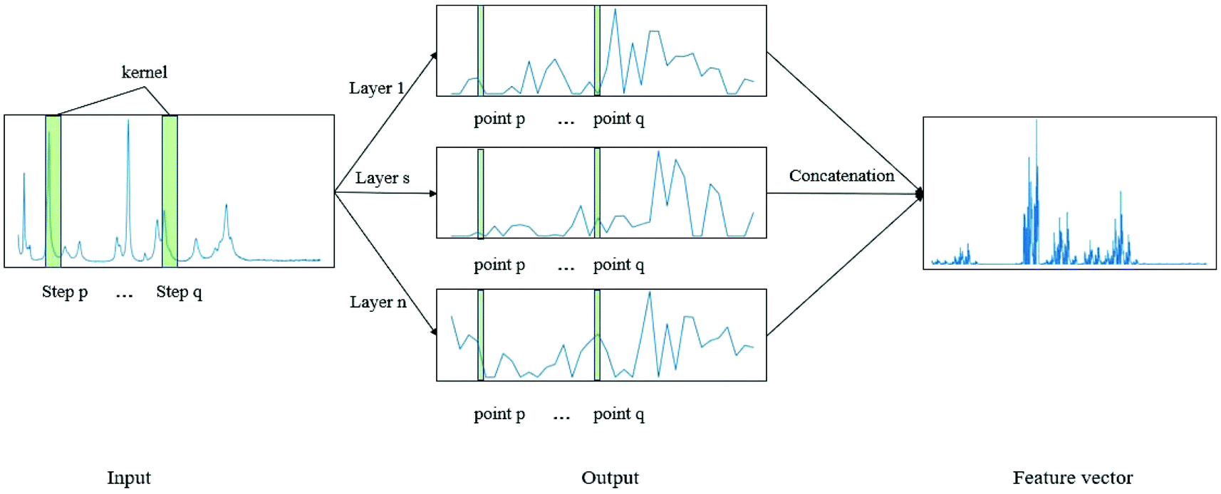 | ||
| Fig. 2 Example showing how the convolution kernel (1 × w) works on a one-layer CNN. The one-dimensional network has one input layer and n output layers. | ||
Rectify linear unit (ReLU) is used as the activation function between layers:
| ReLU = max(0, WTx + b) | (1) |
The SoftMax function is often used in the final layer of a neural network-based classifier. It normalizes the predicted output to obtain the probability distribution on the corresponding class:
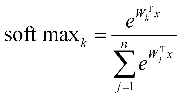 | (2) |
Pooling is another important concept of CNN. It can be regarded as non-linear down-sampling, which can reduce the size of the representation, the number of parameters and the amount of computation.52 The pooling function uses the statistical characteristics (max, in this study) of adjacent outputs at a certain location. For Raman spectra, pooling can provide the translation invariance and increase robustness to peak displacement.
For component identification, CNN can extract the features of the spectra and learn to identify compounds under complex interferences. Since each Raman spectrum can be regarded as a one-dimensional vector, a four-layered one-dimensional CNN is used. The convolutional layers are used to extract the spectral features, and the fully connected layers (1024 and 2 nodes) are used to build the relationship between the feature maps and the existence of the compound. Following each convolution layer, a pooling function is used to improve the learning efficiency. In each convolutional layer and fully connected layer, dropout is applied to prevent overfitting. The architecture of CNN that we have used herein is shown in Fig. 1.
As abovementioned, ReLU and Softmax are used as activation functions. The adaptive moment estimation (Adam)53 is used to train the networks since it requires little memory and has high computational efficiency. It is invariant to diagonal rescaling of the gradients and is well suited for problems that have a large amount of data. Cross entropy loss was used as the loss function. The weights of the network for kernels were initialized by truncated normal distribution, and biases were initialized by the constant of 0.1. Specifically, the bias from 0.01 to 1.00 was considered. The learning rate was 10−4, and the batch size was 100 after optimization. The epoch was in the range from 200 to 300 for models of different components. The criterion for selecting epochs was that the increase of epoch had no obvious contribution to accuracy. The accuracy-epoch curve and loss-epoch curve are shown in Fig. 3 (taking tri(hydroxymethyl)aminomethane as an example, and the other 166 models also achieved similar results by running the code in our GitHub repository).
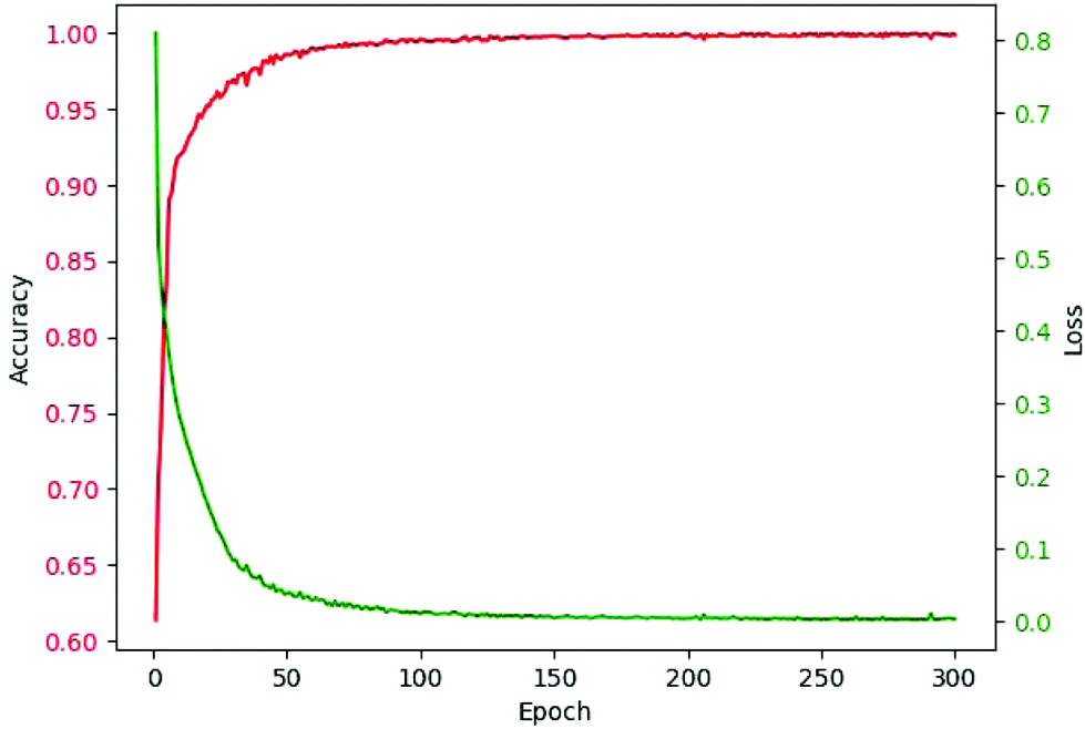 | ||
| Fig. 3 Accuracy-epoch and loss-epoch curves of a valid set during training (using tri(hydroxymethyl)aminomethane as an example). | ||
2.5 Measurement of the prediction quality
Accuracy (ACC), true positive rate (TPR, sensitivity) and false positive rate (FPR, specificity) were used to evaluate the performance of the models in this study. The formulae for ACC, TPR and FPR are as follows: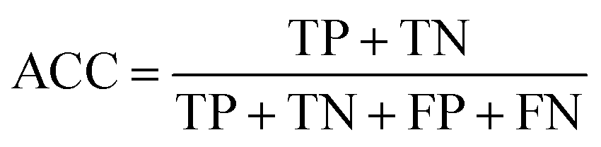 | (3) |
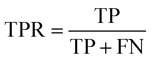 | (4) |
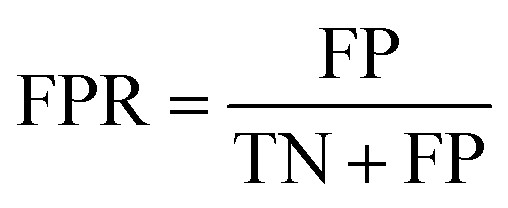 | (5) |
2.6 Computing facilities and implementation
DeepCID was implemented in Python programming language and based on NumPy, SciPy and TensorFlow, and it is available at https:github.com/xiaqiong/DeepCID. Training of the CNN models was accelerated on NVidia GeForce GTX Titan X. The operating system was Windows 10 with an Intel Core i9-7900X processor and 32G DDR4 memory.3. Results and discussion
3.1 Accuracy of the simulated test sets
Table 2 shows the results of the test sets of the simulated datasets. DeepCID achieved significantly better accuracy than k-nearest neighbor (kNN) and back propagation artificial neural network (BP-ANN)54 for the 2500 simulated test samples of each compound. It also improved the results from random forest (RF) and FCNN. DeepCID has almost the same accuracy as logistic regression (LR) with L1-regularization on one-component identification models. The receiver operating characteristic (ROC) curves of different methods are provided in Fig. 4 (tri(hydroxymethyl)aminomethane has been taken as an example, and the other 166 models have provided similar results by running the code in our GitHub repository). As can be seen from the ROC curves, the curve of DeepCID completely encloses the curves of the other methods. The ROC curve of LR with L1-regularization is close to that for DeepCID; this means that their performances are significantly better than those of the other methods. Herein, the BP-ANN models were conventional two-layer fully connected neural networks. After optimization, the number of hidden nodes in BP-ANNs was 40. The Sigmoid55 was used as the activation function, the mean squared error (MSE) was used as the loss function and the stochastic gradient descent56 was used as the optimizer. FCNN models were established by simply removing the convolutional layers of the CNN models. The Adam, ReLU and softmax were used to train the model of FCNN, just like DeepCID. For the accuracy of other compounds in the database, please see Table S1 in the ESI† for more details.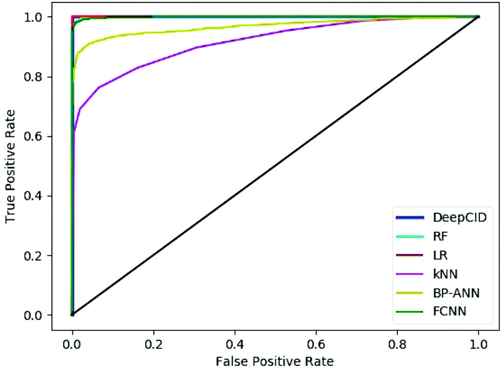 | ||
| Fig. 4 Receiver operating characteristic curves of the different methods (taking tri(hydroxymethyl)aminomethane as an example). | ||
| Model | DeepCID | RF | LR | kNN | BP-ANN | FCNN |
|---|---|---|---|---|---|---|
| Methanol | 99.2 | 98.7 | 99.7 | 91.2 | 96.7 | 98.7 |
| Ethanol | 99.5 | 98.4 | 99.7 | 82.8 | 98.2 | 98.5 |
| Acetonitrile | 99.6 | 98.4 | 99.7 | 82.2 | 95.0 | 99.2 |
| Polyacrylamide | 99.7 | 98.2 | 99.6 | 73.7 | 91.0 | 97.7 |
| Sodium acetate | 99.9 | 98.9 | 99.8 | 82.3 | 97.0 | 98.7 |
| Sodium carbonate | 99.9 | 98.2 | 99.8 | 77.6 | 90.4 | 99.0 |
3.2 Prediction result of the liquid and powder mixture dataset
Herein, six mixtures were analysed to verify the performance of DeepCID. The results are shown in Table 3. The detailed results of DeepCID are listed in Table 1. It can be seen that DeepCID can predict the existence of compounds in these mixtures with high TPR and low FPR. DeepCID, LR with L1-regularization and RF achieve 100% sensitivity (TPR). In fact, TPR reached 100% for each sample; this indicated that DeepCID found all the components existing in the mixtures. FPR reached 0.0%; this indicated that DeepCID had no false-positives on the liquid and powder mixture dataset. In contrast, RF had 8, LR with L1-regularization had 24, kNN had 224, BP-ANN had 37 and FCNN had 70 false-positives. Please see Table 3 for more details.| No. | TPR | FP | ||||||||||
|---|---|---|---|---|---|---|---|---|---|---|---|---|
| DeepCID | RF | LR | kNN | BP-ANN | FCNN | DeepCID | RF | LR | kNN | BP-ANN | FCNN | |
| 1 | 3/3 | 3/3 | 3/3 | 3/3 | 3/3 | 3/3 | 0 | 2 | 5 | 37 | 3 | 1 |
| 2 | 3/3 | 3/3 | 3/3 | 3/3 | 2/3 | 3/3 | 0 | 0 | 4 | 23 | 3 | 0 |
| 3 | 3/3 | 3/3 | 3/3 | 3/3 | 3/3 | 3/3 | 0 | 1 | 5 | 28 | 4 | 2 |
| 4 | 2/2 | 2/2 | 2/2 | 2/2 | 2/2 | 2/2 | 0 | 1 | 4 | 46 | 15 | 33 |
| 5 | 3/3 | 3/3 | 3/3 | 1/3 | 3/3 | 3/3 | 0 | 1 | 2 | 43 | 6 | 13 |
| 6 | 3/3 | 3/3 | 3/3 | 1/3 | 3/3 | 2/3 | 0 | 3 | 4 | 47 | 12 | 21 |
| Statistic | 1.00 | 1.00 | 1.00 | 0.78 | 0.94 | 0.94 | 0 | 8 | 24 | 224 | 37 | 70 |
3.3 Sensitivity of DeepCID at low concentrations
Herein, ninety-four ternary mixture samples with different percentages were used to investigate the sensitivity of DeepCID. The results (Table 4) showed that 91 samples were correctly identified by DeepCID, and only 3 samples with the lowest percentage of methanol (1%) were not identified. Moreover, FCNN correctly detected the presence of methanol only with a percentage above 13%, and LR with L1-regularization, BP-ANN, RF and kNN detected the presence of methanol only with a percentage above 16%, 20%, 23% and 33%, respectively. Thus, DeepCID has better sensitivity when compared with RF, LR with L1-regularization, kNN, BP-ANN and FCNN, especially when the concentration of the compound is low.| Percentage of methanol (%) | Volume of methanol/mL | Volume of acetonitrile/mL | Volume of distilled water/mL | DeepCID | RF | LR | kNN | BP-ANN | FCNN | ||||||||||||
|---|---|---|---|---|---|---|---|---|---|---|---|---|---|---|---|---|---|---|---|---|---|
| a ✓ represents that methanol can be detected by the corresponding method. ‘×’ represents that methanol cannot be detected by the corresponding method. | |||||||||||||||||||||
| 1 | 0.5 | 0/10/20 | 49.5/39.5/29.5 | × | × | × | × | × | × | × | × | × | × | × | × | × | × | × | × | × | × |
| 4 | 2.0 | 0/10/20 | 48/38/28 | ✓ | ✓ | ✓ | × | × | × | √ | × | × | × | × | × | √ | × | × | × | × | × |
| 7 | 3.5 | 0/10/20 | 46.5/36.5/26.5 | ✓ | ✓ | ✓ | × | × | × | √ | × | × | × | × | × | √ | × | × | √ | × | × |
| 10 | 5.0 | 0/10/20 | 45/35/25 | ✓ | ✓ | ✓ | × | × | × | √ | √ | × | √ | × | × | √ | √ | × | √ | √ | × |
| 13 | 6.5 | 0/10/20 | 43.5/33.5/23.5 | ✓ | ✓ | ✓ | × | × | × | √ | √ | × | √ | × | × | √ | √ | × | √ | √ | √ |
| 16 | 8.0 | 0/10/20 | 42/32/22 | ✓ | ✓ | ✓ | × | × | ✓ | √ | √ | √ | √ | × | × | √ | √ | × | √ | √ | √ |
| 20 | 10.0 | 0/10/20 | 40/30/20 | ✓ | ✓ | ✓ | × | × | ✓ | √ | √ | √ | √ | × | × | √ | √ | √ | √ | √ | √ |
| 23 | 11.5 | 0/10/20 | 38.5/28.5/18.5 | ✓ | ✓ | ✓ | ✓ | ✓ | ✓ | √ | √ | √ | √ | √ | × | √ | √ | √ | √ | √ | √ |
| 26 | 13.0 | 0/10/20 | 37/27/17 | ✓ | ✓ | ✓ | ✓ | ✓ | ✓ | √ | √ | √ | √ | √ | × | √ | √ | √ | √ | √ | √ |
| 30 | 15.0 | 0/10/20 | 35/25/15 | ✓ | ✓ | ✓ | ✓ | ✓ | ✓ | √ | √ | √ | √ | √ | × | √ | √ | √ | √ | √ | √ |
| 33 | 16.5 | 0/5/10 | 33.5/28.5/22.5 | ✓ | ✓ | ✓ | ✓ | ✓ | ✓ | √ | √ | √ | √ | √ | √ | √ | √ | √ | √ | √ | √ |
| 36 | 18.0 | 0/5/10 | 32/27/22 | ✓ | ✓ | ✓ | ✓ | ✓ | ✓ | √ | √ | √ | √ | √ | √ | √ | √ | √ | √ | √ | √ |
| 40 | 20.0 | 0/5/10 | 30/25/20 | ✓ | ✓ | ✓ | ✓ | ✓ | ✓ | √ | √ | √ | √ | √ | √ | √ | √ | √ | √ | √ | √ |
| 43 | 21.5 | 0/5/10 | 28.5/23.5/18.5 | ✓ | ✓ | ✓ | ✓ | ✓ | ✓ | √ | √ | √ | √ | √ | √ | √ | √ | √ | √ | √ | √ |
| 46 | 23.0 | 0/5/10 | 27/22/17 | ✓ | ✓ | ✓ | ✓ | ✓ | ✓ | √ | √ | √ | √ | √ | √ | √ | √ | √ | √ | √ | √ |
| 50 | 25.0 | 0/5/10 | 25/20/15 | ✓ | ✓ | ✓ | ✓ | ✓ | ✓ | √ | √ | √ | √ | √ | √ | √ | √ | √ | √ | √ | √ |
| 53 | 26.5 | 0/5/10 | 23.5/18.5/13.5 | ✓ | ✓ | ✓ | ✓ | ✓ | ✓ | √ | √ | √ | √ | √ | √ | √ | √ | √ | √ | √ | √ |
| 56 | 28.0 | 0/5/10 | 22/17/12 | ✓ | ✓ | ✓ | ✓ | ✓ | ✓ | √ | √ | √ | √ | √ | √ | √ | √ | √ | √ | √ | √ |
| 60 | 30.0 | 0/5/10 | 20/15/10 | ✓ | ✓ | ✓ | ✓ | ✓ | ✓ | √ | √ | √ | √ | √ | √ | √ | √ | √ | √ | √ | √ |
| 63 | 31.5 | 0/5/10 | 18.5/13.5/8.5 | ✓ | ✓ | ✓ | ✓ | ✓ | ✓ | √ | √ | √ | √ | √ | √ | √ | √ | √ | √ | √ | √ |
| 66 | 33.0 | 0/2/5 | 17/15/12 | ✓ | ✓ | ✓ | ✓ | ✓ | ✓ | √ | √ | √ | √ | √ | √ | √ | √ | √ | √ | √ | √ |
| 70 | 35.0 | 0/2/5 | 15/13/10 | ✓ | ✓ | ✓ | ✓ | ✓ | ✓ | √ | √ | √ | √ | √ | √ | √ | √ | √ | √ | √ | √ |
| 73 | 36.5 | 0/2/5 | 13.5/11.5/8.5 | ✓ | ✓ | ✓ | ✓ | ✓ | ✓ | √ | √ | √ | √ | √ | √ | √ | √ | √ | √ | √ | √ |
| 76 | 38.0 | 0/2/5 | 12/10/7 | ✓ | ✓ | ✓ | ✓ | ✓ | ✓ | √ | √ | √ | √ | √ | √ | √ | √ | √ | √ | √ | √ |
| 80 | 40.0 | 0/2/5 | 10/8/5 | ✓ | ✓ | ✓ | ✓ | ✓ | ✓ | √ | √ | √ | √ | √ | √ | √ | √ | √ | √ | √ | √ |
| 83 | 41.5 | 0/2/5 | 8.5/6.5/3.5 | ✓ | ✓ | ✓ | ✓ | ✓ | ✓ | √ | √ | √ | √ | √ | √ | √ | √ | √ | √ | √ | √ |
| 86 | 43.0 | 0/2/5 | 7/5/2 | ✓ | ✓ | ✓ | ✓ | ✓ | ✓ | √ | √ | √ | √ | √ | √ | √ | √ | √ | √ | √ | √ |
| 90 | 45.0 | 0/2/5 | 5/3/0 | ✓ | ✓ | ✓ | ✓ | ✓ | ✓ | √ | √ | √ | √ | √ | √ | √ | √ | √ | √ | √ | √ |
| 93 | 46.5 | 0/1/3.5 | 3.5/2.5/0 | ✓ | ✓ | ✓ | ✓ | ✓ | ✓ | √ | √ | √ | √ | √ | √ | √ | √ | √ | √ | √ | √ |
| 96 | 48.0 | 0/1/2 | 2/1/0 | ✓ | ✓ | ✓ | ✓ | ✓ | ✓ | √ | √ | √ | √ | √ | √ | √ | √ | √ | √ | √ | √ |
| 99 | 49.5 | 0/0.25/0.5 | 0.5/0.25/0 | ✓ | ✓ | ✓ | ✓ | ✓ | ✓ | √ | √ | √ | √ | √ | √ | √ | √ | √ | √ | √ | √ |
| 100 | 50.0 | 0 | 0 | ✓ | ✓ | ✓ | ✓ | ✓ | ✓ | ||||||||||||
3.4 Advantages of DeepCID for component identification
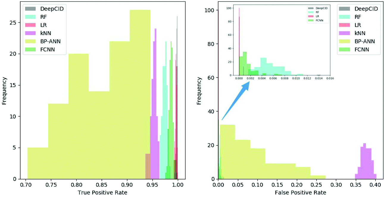
All 167 component identification models of DeepCID achieved an accuracy of 98.8% or better in the augmented test sets, and 160 of them achieved accuracy over 99.5% (Table S1†). This high accuracy ensures the excellent performance of DeepCID in component identification for mixtures.DeepCID had excellent results of TPR and FPR, and Fig. 5 shows an example of the statistical result (tri(hydroxymethyl)aminomethane is taken as an example, and the other 166 components have also achieved similar results by running the code in our GitHub repository). Moreover, one hundred times of sample partitions and trainings were performed for different models to obtain the histograms of TPR and FPR. Obviously, the TPR distribution of DeepCID is closer to 1.0 than that of the other methods. The FPR of DeepCID is closer to 0.0 than that of RF, kNN, BP-ANN and FCNN. Although the distribution of FPR of LR is close to that of DeepCID, DeepCID has a better performance in the other data sets (such as the liquid and powder mixture dataset and ternary mixture dataset.).
 | ||
| Fig. 5 Histograms of TPR (left) and FPR (right) for the different models (taking tri(hydroxymethyl)aminomethane as an example). One hundred times of sample partitions and trainings were performed for the different models. | ||
As abovementioned, the training datasets were generated randomly based on the database. The spectra in the training datasets contained not only the noise of the original spectra, but also the interference of other compounds. Moreover, the liquid and powder and ternary mixture datasets were acquired using different Raman spectrometers. In this situation, DeepCID achieved excellent identification, with no false positive and false negative errors. This means that DeepCID not only can alleviate the noise interference (different background), but also the interference of other compounds.
In fact, DeepCID can also alleviate the displacement in Raman shifts and the variation in Raman intensity between different instruments. Taking the pure spectrum of methanol as an example, it can be observed clearly in Fig. 6 that the Raman peaks shift from 1034 and 1452 cm−1 (database) to 1036 and 1454 cm−1 (ternary mixture dataset), respectively. In addition, the maximum intensity of 100% methanol from the ternary mixture dataset was nearly two times higher than that from the database. In this case, DeepCID accurately identified methanol in mixtures in the ternary mixture dataset. This is strong evidence that DeepCID has great capability to correct Raman shifts and Raman intensity.
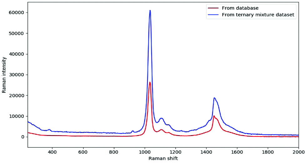 | ||
| Fig. 6 Comparison of 100% methanol from the database and ternary mixture dataset. | ||
DeepCID showed excellent sensitivity, especially at low concentrations. It effectively identified methanol mixtures with a percentage as low as 4% in the ternary mixture dataset. Thus, compared with the other methods used (FCNN correctly detected the presence of methanol with a percentage above 13%, and LR with L1-regularization, BP-ANN, RF and kNN correctly detected the presence of methanol with a percentage above 16%, 20%, 23% and 33%, respectively), it undoubtedly has great advantages and improvement.
NVidia GeForce GTX Titan X GPU was used to accelerate the training of CNNs. In 300 epochs, it took about five minutes for training. During the prediction, reloading one model and making prediction consumed less than one second. Specifically, the analysis of 6 mixture spectra with 167 CNN was completed within two minutes. If these 167 models could be preloaded into the memory, the prediction would be finished within only one second for the 6 mixture spectra. Therefore, DeepCID is efficient enough to identify components in mixtures.
Currently, DeepCID can be viewed as a pre-training model. When new samples are available for training, DeepCID can easily be further evolved to achieve better accuracy since all training samples are generated by augmentation from the database. If there are real samples for fine-tuning, DeepCID will achieve even better performance.
With DeepCID, the pre-processing process can be avoided. It not only simplifies the pipeline of DeepCID, but also avoids introduction of errors and variations from pre-processing. To compare and further prove that DeepCID does not require pre-processing, pre-processed data has also been used to build models such as DeepCID. Whittaker smoother57 and adaptive iteratively reweighted Penalized Least Squares (airPLS)51,58 were used to smooth and correct the baseline of the Raman spectra. Some of the results are listed in Tables S2 and S3.† The comparison results show that although the pre-processing improved the fitting accuracy, it also reduced the generalization ability of the models. Specifically, DeepCID with pre-processing increases the probability of false-positive errors and false-negative errors.
3.5 The function of the convolutional layers
To verify that the convolution layers play an important role in the spectral feature extraction and component identification, the convolution layers have been removed from DeepCID. In fact, the network without convolution layers is equivalent to a double-layered fully connected network, which is called FCNN herein. After adjustment of the architecture of the model and optimization of its parameters, the results of FCNN are shown in Table 2. Obviously, DeepCID had higher accuracy than FCNN. This means that the convolution layers play an important role in feature extraction and component identification.3.6 Stability and reproducibility
In deep learning, parameters are often initialized randomly, and random dropouts are presented too, which result in some randomness of the results. Thus, to verify the stability of DeepCID for component identification, we selected models of acetonitrile and methanol to perform multiple trainings. One hundred trainings were performed for both compounds. The prediction accuracy of the 2500 samples of the test dataset was used to evaluate the stability. The histograms of accuracy are shown in Fig. 7, which show that DeepCID has great stability. The distributions of accuracy approximate Gaussian distributions with small variances.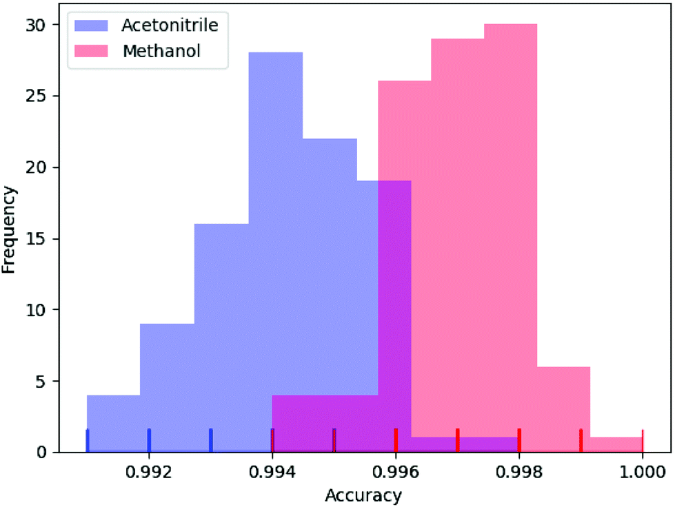 | ||
| Fig. 7 Stability and reproducibility of DeepCID. One hundred trainings were performed for the models of acetonitrile and methanol on simulated test set. | ||
4. Conclusions
In this study, DeepCID models were developed for Raman spectra based on deep learning techniques. Simulated, liquid and powder mixtures and ternary mixtures datasets were used to evaluate its performance. The results show that DeepCID can achieve better accuracy when compared with LR with L1-regularization, kNN, RF, BP-ANN and FCNN. DeepCID had no false-negatives and false-positives in all the liquid and powder mixture samples. Moreover, DeepCID showed the best sensitivity, and it could detect mixtures with volume percentage of methanol as low as 4%. In contrast, LR with L1-regularization could only detect mixtures with a volume percentage of methanol above 16%, and RF, BP-ANN, FCNN, and kNN could only detect mixtures with a volume percentage of methanol above 23%, 20%, 13% and 33%, respectively. The identification results are significantly better when compared with those obtained from other methods. It was verified that convolution layers played a crucial role in feature extraction. DeepCID models have been developed based on TensorFlow, which can make full use of GPU and learn effectively from a large number of spectra. It can also be further fine-tuned for better performance if more datasets are available. Thus, it is a promising component identification technique for Raman spectroscopy. In this study, DeepCID was established based on a pure compound Raman spectra database. However, the pipeline of DeepCID is universal and portable. For example, for some diseases with metabolomic biomarkers, DeepCID models may be constructed for quick diagnosis of these diseases.Conflicts of interest
There are no conflicts to declare.Acknowledgements
This work was financially supported by the National Natural Science Foundation of China (Grant No. 21675174, 21873116 and 21305163). The studies meet with the approval of the university's review board. We are grateful to all employees of this institute for their encouragement and support for this research.References
- M. Yang, Y. Sun, X. Zhang, B. Mccord, A. J. Mcgoron, A. Mebel and Y. Cai, Talanta, 2017, 179, 520–530 CrossRef PubMed.
- K. Kneipp, H. Kneipp, I. Itzkan, R. R. Dasari and M. S. Feld, Chem. Rev., 1999, 30, 2957–2976 CrossRef.
- K. Carron and R. Cox, Anal. Chem., 2010, 82, 3419–3425 CrossRef PubMed.
- R. Y. Satoberrú, J. Medinavaltierra, C. Medinagutiérrez and C. Fraustoreyes, Spectrochim. Acta, Part A, 2004, 60, 2225–2229 CrossRef PubMed.
- Z. P. Chen, L. M. Li, J. W. Jin, A. Nordon, D. Littlejohn, J. Yang, J. Zhang and R. Q. Yu, Anal. Chem., 2012, 84, 4088–4094 CrossRef CAS PubMed.
- W. Zhou, Y. Ying and L. Xie, Appl. Spectrosc. Rev., 2012, 47, 654–670 CrossRef.
- P. Vandenabeele, L. Moens, H. G. M. Edwards and R. Dams, J. Raman Spectrosc., 2000, 31, 509–517 CrossRef CAS.
- L. Burgio and R. J. Clark, Spectrochim. Acta, Part A, 2001, 57, 1491–1521 CrossRef CAS.
- K. Castro, M. Pérez-Alonso, M. D. Rodríguez-Laso, L. A. Fernández and J. M. Madariaga, Anal. Bioanal. Chem., 2005, 382, 248–258 CrossRef CAS PubMed.
- J. D. Gelder, K. D. Gussem, P. Vandenabeele and L. Moens, J. Raman Spectrosc., 2007, 38, 1133–1147 CrossRef.
- J. Hwang, N. Choi, A. Park, J. Q. Park, H. C. Jin, S. Baek, S. G. Cho, S. J. Baek and J. Choo, J. Mol. Struct., 2013, 1039, 130–136 CrossRef CAS.
- Z. M. Zhang, X. Q. Chen, H. M. Lu, Y. Z. Liang, W. Fan, D. Xu, J. Zhou, F. Ye and Z. Y. Yang, Chemom. Intell. Lab. Syst., 2014, 137, 10–20 CrossRef CAS.
- S. Lee, H. Lee and H. Chung, Anal. Chim. Acta, 2013, 758, 58–65 CrossRef CAS PubMed.
- S. S. Khan and M. G. Madden, Chemom. Intell. Lab. Syst., 2012, 114, 99–108 CrossRef CAS.
- J. D. Rodriguez, B. J. Westenberger, L. F. Buhse and J. F. Kauffman, Anal. Chem., 2011, 83, 4061–4067 CrossRef CAS PubMed.
- P. Vandenabeele, H. An, H. G. M. Edwards and L. Moens, Appl. Spectrosc., 2001, 55, 525–533 CrossRef CAS.
- V. A. Shashilov and I. K. Lednev, Chem. Rev., 2010, 110, 5692–5713 CrossRef CAS PubMed.
- J. R. Ferraro, K. Nakamoto and C. W. Brown, Introductory Raman Spectroscopy, Academic Press, Cambridge, 2nd edn, 2003 Search PubMed.
- W. Windig, J. Guilment and A. Chem, Anal. Chem., 1991, 63, 1425–1432 CrossRef CAS.
- Y. S. Su, E. Widjaja, L. E. Yu and M. Garland, J. Raman Spectrosc., 2003, 34, 795–805 CrossRef.
- J. J. González-Vidal, R. Perez-Pueyo, M. J. Soneira and S. Ruiz-Moreno, J. Raman Spectrosc., 2012, 43, 1707–1712 CrossRef.
- T. Vignesh, S. Shanmukh, M. Yarra, E. Botonjic-Sehic, J. Grassi, H. Boudries and S. Dasaratha, Appl. Spectrosc., 2012, 66, 334–340 CrossRef CAS PubMed.
- D. Wu, M. Yaghoobi, S. Kelly, M. Davies and R. Clewes, Sensor Signal Processing for Defence, IEEE, Edinburgh, 2014 Search PubMed.
- K. R. Coombes, K. A. Baggerly and J. S. Morris, Pre-Processing Mass Spectrometry Data, Springer, US, New York, 2007 Search PubMed.
- K. H. Liland, T. Almøy and B. H. Mevik, Appl. Spectrosc., 2010, 64, 1007–1016 CrossRef CAS PubMed.
- Y. Lecun, Y. Bengio and G. Hinton, Nature, 2015, 521, 436–444 CrossRef CAS PubMed.
- J. Acquarelli, L. T. Van, J. Gerretzen, T. N. Tran, L. M. Buydens and E. Marchiori, Anal. Chim. Acta, 2017, 954, 22–31 CrossRef CAS PubMed.
- J. Liu, M. Osadchy, L. Ashton, M. Foster, C. J. Solomon and S. J. Gibson, Analyst, 2017, 142, 4067–4074 RSC.
- C. Cui and T. Fearn, Chemom. Intell. Lab. Syst., 2018, 182, 9–20 CrossRef CAS.
- S. L. Neal, Appl. Spectrosc., 2018, 72, 102–113 CrossRef CAS PubMed.
- S. Malek, F. Melgani and Y. Bazi, J. Chemom., 2017, 32, e2977 CrossRef.
- N. H. Tran, X. Zhang, L. Xin, B. Shan and M. Li, Proc. Natl. Acad. Sci. U. S. A., 2017, 114, 8247–8252 CrossRef CAS PubMed.
- X. X. Zhou, W. F. Zeng, H. Chi, C. Luo, C. Liu, J. Zhan, S. M. He and Z. Zhang, Anal. Chem., 2017, 89, 12690–12697 CrossRef CAS PubMed.
- S. Wang, S. Fei, Z. Wang, Y. Li, J. Xu, F. Zhao and X. Gao, Bioinformatics DOI:10.1093/bioinformatics/bty684.
- P. Inglese, J. S. Mckenzie, A. Mroz, J. Kinross, K. Veselkov, E. Holmes, Z. Takats, J. K. Nicholson and R. C. Glen, Chem. Sci., 2017, 8, 3500–3511 RSC.
- M. Wen, Z. Zhang, S. Niu, H. Sha, R. Yang, Y. Yun and H. Lu, J. Proteome Res., 2017, 16, 1401–1409 CrossRef CAS PubMed.
- M. Wen, P. Cong, Z. Zhang, H. Lu and T. Li, Bioinformatics, 2018, 34, 3781–3787 CrossRef PubMed.
- D. Jiang, S. Malla, Y. J. Fu, D. Choudhary and J. F. Rusling, Anal. Chem., 2017, 89, 12872–12879 CrossRef CAS PubMed.
- D. H. Hubel and T. N. Wiesel, J. Physiol., 1962, 160, 106–154 CrossRef CAS.
- K. Fukushima, Neural Networks, 1988, 1, 119–130 CrossRef.
- Q. Zhang and A. Benveniste, IEEE Trans. Neural Networks, 1992, 3, 889–898 CrossRef CAS PubMed.
- Y. L. Cun, B. Boser, J. S. Denker, R. E. Howard, W. Habbard, L. D. Jackel and D. Henderson, Adv. Neural Inf. Process. Syst., 1990, 2, 396–404 Search PubMed.
- Y. Lecun, L. Bottou, Y. Bengio and P. Haffner, Proc. IEEE, 1998, 86, 2278–2324 CrossRef.
- A. Krizhevsky, I. Sutskever and G. E. Hinton, NIPS'12 Proceedings of the 25th International Conference on Neural Information Processing Systems, Curran Associates Inc, New York, 2012 Search PubMed.
- V. Nair and G. E. Hinton, ICML'10 Proceedings of the 27th International Conference on Machine Learning, Omnipress, Madison, 2010 Search PubMed.
- N. Srivastava, G. Hinton, A. Krizhevsky, I. Sutskever and R. Salakhutdinov, J. Machine Learning Res., 2014, 15, 1929–1958 Search PubMed.
- M. D. Zeiler and R. Fergus, Computer Vision-ECCV 2014, Springer International Publishing, Heidelberg, 2014 Search PubMed.
- K. Simonyan and A. Zisserman, The 3rd International Conference for Learning Representations, ICLR, San Diego, 2015 Search PubMed.
- C. Szegedy, W. Liu, Y. Jia, P. Sermanet, S. Reed, D. Anguelov, D. Erhan, V. Vanhoucke and A. Rabinovich, 2015 IEEE Conference on Computer Vision and Pattern Recognition, IEEE, Piscataway, 2015 Search PubMed.
- T. Wang, D. J. Wu, A. Coates and A. Y. Ng, Proceedings of the 21st International Conference on Pattern Recognition, IEEE, Piscataway, 2012 Search PubMed.
- Z. M. Zhang, S. Chen and Y. Z. Liang, Analyst, 2010, 135, 1138–1146 RSC.
- I. Goodfellow, Y. Bengio and A. Courville, Deep Learning, The MIT Press, Cambridge, 2016 Search PubMed.
- D. Kingma and J. Ba, The 3rd International Conference for Learning Representations, ICLR, San Diego, 2015 Search PubMed.
- D. E. Rumelhart, G. E. Hinton and R. J. Williams, Nature, 1986, 323, 399–421 CrossRef.
- J. Han and C. Moraga, IWANN ‘96 Proceedings of the International Workshop on Artificial Neural Networks: From Natural to Artificial Neural Computation, Springer-Verlag, London, 1995 Search PubMed.
- L. Bottou, Proceedings of COMPSTAT'2010, Physica-Verlag, Heidelberg, 2010 Search PubMed.
- P. H. Eilers, Anal. Chem., 2003, 75, 3631–3636 CrossRef CAS PubMed.
- Z. M. Zhang and Y. Z. Liang, Chromatographia, 2012, 75, 313–314 CrossRef CAS.
Footnote |
| † Electronic supplementary information (ESI) available. See DOI: 10.1039/c8an02212g |
| This journal is © The Royal Society of Chemistry 2019 |