
 Open Access Article
 This Open Access Article is licensed under a
 Creative Commons Attribution 3.0 Unported Licence
Quantitative profile–profile relationship (QPPR) modelling: a novel machine learning approach to predict and associate chemical characteristics of unspent ammunition from gunshot residue (GSR)†
Matteo D.
Gallidabino
 *a,
Leon P.
Barron
b,
Céline
Weyermann
c and
Francesco S.
Romolo
de
*a,
Leon P.
Barron
b,
Céline
Weyermann
c and
Francesco S.
Romolo
de
aCentre for Forensic Science, Department of Applied Sciences, Faculty of Health & Life Sciences, Northumbria University Newcastle, Ellison Building, NE1 8ST Newcastle Upon Tyne, UK. E-mail: matteo.gallidabino@northumbria.ac.uk; Tel: +44 (0)191 227 4859
bKing's Forensics, Division of Analytical, Environmental & Forensic Sciences, Faculty of Life Sciences and Medicine, King's College London, 150 Stamford Street, SE1 9NH London, UK
cÉcole des Sciences Criminelles, Faculté de Droit, des Sciences Criminelles et d'Administration Publique, Université de Lausanne, Bâtiment Batochime, 1015 Lausanne-Dorigny, Switzerland
dSezione di Medicina Legale, Dipartimento SAIMLAL, Sapienza Università di Roma, Viale Regina Elena 336, 00161 Rome, Italy
eFacultade de Química, Universidade de Santiago de Compostela, Avda. das Ciencias, s/n. Campus sur, 15782 Santiago de Compostela, Spain
First published on 2nd November 2018
Abstract
Evidence association in forensic cases involving gunshot residue (GSR) remains very challenging. Herein, a new in silico approach, called quantitative profile–profile relationship (QPPR) modelling, is reported. This is based on the application of modern machine learning techniques to predict the pre-discharge chemical profiles of selected ammunition components from those of the respective post-discharge GSR. The obtained profiles can then be compared with one another and/or with other measured profiles to make evidential links during forensic investigations. In particular, the approach was optimised and successfully tested for the prediction of GC-MS profiles of smokeless powders (SLPs) from organic GSR in spent cases, for nine ammunition types. Results showed a high degree of similarity between predicted and experimentally measured profiles, after adequate combination and evaluation of fourteen machine learning techniques (median correlation of 0.982). Areas under the curve (AUCs) of 0.976 and 0.824 were observed after receiver operating characteristic (ROC) analysis of the results obtained in the comparisons between predicted–predicted and predicted–measured profiles, respectively, in the specific case that the ammunition types of interest were excluded from the training dataset (i.e., extrapolation). Furthermore, AUCs of 0.962 and 0.894 were observed in interpolation mode. These values were close to those of the comparison of the measured SLP profiles between themselves (AUC = 0.998), demonstrating excellent potential to correctly associate evidence in a number of different forensic scenarios. This work represents the first time that a quantitative approach has successfully been applied to associate a GSR to a specific ammunition.
1. Introduction
Association is a key challenge in forensic science.1 In the reconstruction of shooting events, in particular, associating a variety of different entities and/or items discovered during an investigation (as, for example, a spent cartridge case with a reference ammunition or entry hole) may provide law-enforcement authorities with crucial intelligence and scientific evidence.2,3 As bullets and spent cartridges are primarily involved in discharge, they carry physical marks left by the used firearm and other intrinsic features. Thus, special emphasis is usually put on their examination. Their usefulness, however, may be limited in a number of cases. For example, physical characteristics may be poorly selective or not exploitable due to post-discharge deformations, poor impression quality or high frequency in the general population. Moreover, bullets, in particular, may pass through the target and/or be lost to inaccessible locations, whilst spent cartridges may be collected by the perpetrator or simply not released after the discharge (e.g., use of a revolver). Under these circumstances, and several more, alternative pieces of evidence, such as the gunshot residue (GSR), must be exploited.The GSR is the chemical trace systematically released as a secondary effect of a firearm discharge.4–7 It is a heterogeneous mixture of different species containing contribution from all the cartridge elements. The most forensically relevant fractions are the so-called organic GSR (OGSR) and primer GSR (pGSR). The OGSR is primarily the residue from the explosion of the smokeless powder (SLP) and contains both the organic species originally present in it, as well as numerous transformation products. The pGSR is, on the contrary, mainly the residue of the explosion of the primer mixture and is composed of microscopic particles resulting from the condensation of vaporised metals. After discharge, these fractions are released from every opening of the firearm and deposited on surfaces nearby, such as the hands/body of the shooter. A large portion can also reach the target or remain inside the spent cartridge. For these reasons, GSR analysis already finds many successful applications in the investigation of firearm-related crimes,8,9 such as, for example, the identification of persons involved in shooting events, the estimation of shooting distance and/or the time since discharge.
Concerning evidence association, a number of works have explored the possibility to establish links between different GSRs found on a crime scene and/or between a GSR and a specific ammunition or firearm. In this regard, it has been observed that both pGSR and OGSR display large variation between different sources, at micro- and macro-physicochemical levels, in a number of different features, including particle/flake morphology,10,11 chemical composition12–18 and distribution of particle classes.19,20 Through the comparison of quantitative chemical profiles, in particular, grouping different GSR traces released from the same source has been frequently proved to be achievable, as long as these were collected from similar deposition surfaces.21–25 Clustering or classification models, such as hierarchical clustering analysis or linear discriminant analysis, have shown promise for this purpose. Additionally, comparison of qualitative or simple semi-quantitative characteristics, such as the occurrence of certain particle classes or ratios between specific chemical species, has been proved to provide some insight about the general type of ammunition or firearm used.12,26–30
These reported approaches, however, suffer from some important limitations. In particular, association of evidence has essentially been limited to GSRs recovered from the same deposition surface. GSRs released by the same ammunition, but collected at different locations (e.g., spent cartridge cases and target entry holes) were found to potentially differ in their physicochemical characteristics.23,31 Even more importantly, the profiles of GSRs and their original ammunition elements were generally observed to be inconsistent (even if mutually dependent), due to discharge-induced alterations, sampling effects and/or differences in analytical procedures.14,16,32–34 As a result, only the comparison of the basic qualitative or semi-quantitative measurements was possible, which holds a weak association efficacy. When a stronger association needs to be established, indirect comparison is currently carried out. This involves the firing of reference ammunition (for example, seized from the suspect) using the suspected firearm, followed by the analysis and comparison of the reference GSRs deposited on the different surfaces of interest.23 As a trial-and-error procedure, this is time consuming, laborious and depends on the availability of both reference ammunition and firearm. As a consequence, it can be applied only in selected cases.
More flexible, rapid and efficient strategies are required, as highlighted in various recent critical publications.6,8,35 In this regard, the possibility to use statistical methods to quantitatively predict the chemical profiles of the initial cartridge components from those of the respective GSRs (i.e., in silico profiling) may hold significant advantages. This, indeed, would allow rapid and direct comparison between a GSR and a specific ammunition, without requiring shooting tests or analytical procedures. Additionally, it could also enable direct comparisons of GSRs deposited on different surfaces, thus solving inherent limitations of current approaches and providing high association powers, which could flexibly be applied in a number of different situations. Building reliable predictive models, however, is obviously a challenging procedure given the complex combination of variables that may contribute to differences between pre- and post-discharge profiles. Nonetheless, in recent years, deconvolution of highly complex relationships using advanced regression techniques, mainly borrowed from machine learning,36,37 has been extensively demonstrated in a wide range of fields. In the field of chemistry, these have led to the possibility of in silico prediction of a large range of quantitative bio- and physicochemical properties from molecular descriptors. This family of methods collectively fall under the umbrella term of “quantitative structure–activity relationship (QSAR) modelling”.38,39
Herein, a new modelling procedure inspired by QSAR modelling approaches is investigated, specifically developed to model quantitative relationships between GSR and initial cartridge components. This new concept is called “quantitative profile–profile relationship (QPPR) modelling” and involves two steps. Firstly, machine learning techniques are applied to model and deconvolute the complexity of the discharge process, in order to quantitatively predict individual characteristics in the pre-discharge profile of ammunition components of interest (e.g., the peak areas of the different stabilisers in a SLP chromatogram) from the whole post-discharge profile of a GSR. The best models for the different pre-discharge characteristics are then selected and combined in order to assemble a reconstructed profile.
In particular, QPPR has been tested here to predict pre-discharge chromatographic profiles of SLPs from those of the respective OGSRs in spent cartridges. To this end, SLPs and OGSRs from nine different types of ammunition were extracted by solvent extraction (SE) and headspace sorptive extraction (HSSE), respectively, before analysis with gas chromatography-mass spectrometry (GC-MS), to compile a suitable database of pre- and post-discharge profiles for modelling. Output and input compounds were then selected and fourteen different machine learning techniques tested for their ability to quantitatively relate their observed signals. As different machine learning techniques have been shown to have variable performances across different applications,40 QPPR was implemented here in a multimodal approach by combining a number of them together. General validity of the overall QPPR modelling procedure was finally tested on a set of independent external cases. To our knowledge, this work represents the first time that a quantitative approach has successfully been applied to associate OGSRs to their original ammunition. It is also the first time that an in silico profiling approach based on multivariate analysis has been suggested.
2. Experimental
2.1. Materials and equipment
Nine types of ammunition were purchased from different suppliers available in Switzerland. Five of them were of .45 ACP calibre and manufactured by Geco (Ge45), PMC (Pm45), Remington UMC (Re45), Sellier & Bellot (Se45) and Magtech (Ma45). The remaining four were of .357 Magnum calibre and manufactured by Geco (Ge357), Sellier & Bellot (Se357), Samson (Sa357) and Magtech (Ma357). Preliminary analysis revealed that all ammunition types contained double-base SLPs, except Ma45, which contained a single-base SLP. Methanol was of puriss. grade and purchased from Sigma Aldrich (Buchs, Switzerland).An Agilent 7890A gas chromatograph coupled to an Agilent 5975C mass selective detector (Agilent Technologies, Basel, Switzerland) was used for all analyses. This was equipped with a Gerstel CIS-4 programmed temperature vaporising (PTV) injector, as well as a Gerstel TDU thermal desorption unit that was connected on-line to the injector. The system was also equipped with a Gerstel MPS multi-purpose sampler, which was used to automatically inject aliquots of liquid samples into the PTV injector or load tubes containing HSSE stir-bars into the TDU. Liners for CIS-4 were obtained from Gerstel and packed with quartz-wool. Separations were performed on a HP-5MS (30 m × 0.25 mm × 0.25 μm) column from Agilent. The carrier gas was helium.
2.2. Analysis of SLPs and OGSRs
SLPs contained in the different ammunition types were recovered by opening the respective cartridges using a kinetic hammer. SLPs were then extracted and analysed according to a previously reported protocol.41 This involved SE with methanol and direct analysis of the supernatant liquids by GC-MS using a cold split injection technique, in order to minimise degradation of thermo-labile compounds. For each ammunition type, four cartridges from the same ammunition box were opened and analysed (n = 36).In order to obtain OGSR samples, cartridges from the different ammunition types were discharged with different handguns depending on the calibre, i.e. a Colt 1911 semi-automatic pistol (.45 ACP) and a Colt Python revolver (.357 Magnum). For each ammunition type, three cartridges from the same boxes as those used for SLP experiments were sampled at random (n = 27). Test shootings were carried out by singly loading cartridges in the magazine/cylinder. OGSRs were directly recovered from spent cases and analysed according to another previously published protocol.41 Briefly, this involved the headspace extraction of the spent cases in a glass vial for 72 h at 80 °C with high-capacity HSSE stir bars (polydimethylsiloxane, volume of 110 μL). The stir bars were then thermally desorbed in the TDU and volatilised compounds injected on-line onto the GC-MS.
2.3. Descriptor extraction and data pre-treatment
A total of eight compounds were detected in the GC-MS chromatograms of the pre-discharge SLPs. These were all retained as descriptors for the SLP profiles and thus used as outputs (abbreviated with “O”) in QPPR modelling. The eight compounds were: nitroglycerin (ONG, tR = 9. 861 min, m/z = 46), diphenylamine (ODPA, tR = 12.128 min, m/z = 169), ethyl centralite (OEC, tR = 14.138 min, m/z = 120), dibutyl phthalate (ODBP, tR = 14.497 min, m/z = 149), 2-nitrodipihenylamine (O2ND, tR = 14.651 min, m/z = 214), akardite II (OAK2, tR = 14.989 min, m/z = 169), dioctyl fumarate (ODOF, tR = 16.076 min, m/z = 70), and 4-nitrodiphenylamine (O4ND, tR = 16.384 min, m/z = 214).Hundreds of compounds were detected by GC-MS in all OGSRs. Amongst them, eight were specifically selected as descriptors for the OGSR profiles and used as inputs (abbreviated with “I”) in QPPR modelling, i.e. 2-ethyl-1-hexanol (IHEX, tR = 8.508 min, m/z = 57), diphenylamine (IDPA, tR = 21.407 min, m/z = 169), ethyl centralite (IEC, tR = 27.117 min, m/z = 120), dibutyl phthalate (IDBP, tR = 28.426 min, m/z = 149), 2-nitrodiphenylamine (I2ND, tR = 28.506 min, m/z = 214), akardite II (IAK2, tR = 29.512 min, m/z = 169), 4-nitrodiphenylamine (I4ND, tR = 32.374 min, m/z = 214), and 2,4-dinitrodiphenylamine (IDND, tR = 34.353 min, m/z = 259). These eight compounds were mainly chosen because they were either the same as the outcome compounds (i.e., DPA, 2ND, 4ND, AK2, EC and DBP), or directly related to them in terms of their synthesis and/or degradation pathways (i.e., DND and HEX). This made them close in terms of reciprocal dependence, which was likely beneficial for predictive modelling. They also have a higher probability of being detected in OGSRs compared to most of the other analytes. Indeed, previous research reported slower disappearance rates due to lower volatility and, on average, higher measured concentrations in OGSR samples.25
Chromatographic peak areas corresponding to the base ion of each of the aforementioned compounds were extracted using Enhanced Data Analysis software provided by Agilent. These were then transformed into their base-10 logarithms (logPAs). Indeed, this transformation was preliminarily found to significantly reduce distribution skewness and heteroscedasticity. See ESI† for a comparison of data distributions before and after transformation (Tables S1 and S2, as well as Fig. S1 and S2†). For the sake of use in QPPR modelling, output variables were further averaged within each set of four replicate SLP analyses before base-10 logarithm transformation, in order to build consensus profiles to be associated with the respective OGSR analyses. Input variables were centred by subtracting their respective distribution means across the different OGSR analyses and scaled to the standard deviations (i.e., they were standardised). A summary of the compounds selected as variables, along with their respective characteristics, is reported in Table 1.
| Compound | General abbr. | Target ion (m/z) | t R in OGSR method (min) | Input abbr. | t R in SLP method (min) | Output abbr. | Best model |
|---|---|---|---|---|---|---|---|
| Blank spaces indicate that the specific compound was not selected as descriptor for the considered group of profiles. | |||||||
| 2-Ethyl-1-hexanol | HEX | 57 | 8.508 | IHEX | |||
| Nitroglycerin | NG | 46 | 9.861 | ONG | RF-CIT | ||
| Diphenylamine | DPA | 169 | 21.407 | IDPA | 12.128 | ODPA | CR |
| Ethyl centralite | EC | 120 | 27.117 | IEC | 14.138 | OEC | CR |
| Dibutyl phthalate | DBP | 149 | 28.426 | IDBP | 14.497 | ODBP | ANN |
| 2-Nitrodiphenylamine | 2ND | 214 | 28.506 | I2ND | 14.651 | O2ND | CR |
| Akardite II | AK2 | 169 | 29.512 | IAK2 | 14.989 | OAK2 | OLS |
| Dioctyl fumarate | DOF | 70 | 16.076 | ODOF | RF-CIT | ||
| 4-Nitrodiphenylamine | 4ND | 214 | 32.374 | I4ND | 16.384 | O4ND | SVM-RAD |
| 2,4-Dinitrodiphenylamine | DND | 259 | 34.353 | IDND | |||
2.4. Prediction of output compounds
The first step in QPPR modelling involved the prediction of logPAs for the single output compounds. This was performed one by one, using the full set of input compounds each time. The eight outputs were thus treated as mutually independent variables and predicted from of all the inputs taken as a group.Fourteen machine learning-based regression methods were tested (see also Table S3 in ESI†): multinomial ordinary least-squares (OLS), partial least-squares (PLS), ridge regression (RR), elastic net (EN), multivariate adaptive regression splines (MARS), k-nearest neighbors regression (KNN), extreme learning machine (ELM), single-layer feed-forward perceptron neural network (ANN), support vector machines with radial basis function (SVM-RAD) or polynomial function (SVM-POL) as kernels, random forest exploiting classification and regression trees (RF-CART) or conditional inference trees (RF-CIT) algorithms as base learners, boosted trees (BT) and Cubist regression (CR). This specific set of models was selected to cover and test all the main categories of machine learning modelling techniques, such as support vectors, neural-based and tree-based methods. Indeed, different modelling methods have previously been shown to have variable performance in fitting the same dataset.40 This set also allowed comparison of linear (i.e., OLS, PLS, RR and EN) with non-linear methods (MARS, KNN, ELM, ANN, SVM, RF, BT and CR).
Due to their recognised instability, an ensemble approach was applied to MARS and ANN in order to potentially improve predictions. In particular, averaging between five models was used for ANN and bagging between ten models for MARS.
2.5. Training and validation of regression models
Two different training schemes were followed to assess the performance of the QPPR-modelling procedure in different casework scenarios. These were: (1) the case where the developed models were not trained on the OGSR of the ammunition type of interest and the corresponding SLP profile thus needed to be extrapolated (i.e., no replicate analysis for this OGSR was part of the training library); (2) the opposite case where the developed models were trained on the OGSR of the ammunition type of interest and the corresponding SLP profile could be interpolated (i.e., replicate analyses for this OGSR were included in the training library). An extrapolation perspective, in particular, was adopted for method optimisation and selection of best models, as it represents the worst-case forensic scenario.To test prediction performance in extrapolation mode, all three replicate OGSR analyses of a given ammunition were excluded from the training dataset and the models trained on the remaining data, which comprised all OGSR analyses of the remaining eight ammunition types. To test performance in interpolation mode, on the contrary, only one of the three replicate OGSR analyses for a given ammunition was omitted from the training dataset and the models trained on the remaining data, which also included the remaining two OGSR analyses of the same ammunition. In both cases, the procedure was repeated for all the available analyses; the omitted data were used as validation subsets to determine global regression performances.
Model fitting was carried out using R statistical computing software v3.4.1 and the caret package, as described by Kuhn and Johnson.40 All tested regression methods involved at least one tuning parameter, which was optimised during model fitting by resampling of the training subset using a leave-one-out cross-validation procedure. The root-mean-square error (RMSE) of predicted logPAs was used to assess global prediction performance. See Table S3 in ESI† for details about models, related algorithms, tuning parameters and specific R packages. For further model assessment, linearity between each output and the full set of inputs was measured through the coefficients of determination (R2) of their respective OLS models, inferred from the complete dataset of analyses, without left out. Input importance on the prediction of the different outputs was determined using the internal scoring method of RF-CART. This automatically ranked inputs as a function of their impact on regression and returned a relative importance factor.
2.6. Assembly and comparison of profiles
For each OGSR analysis used in model validation, predicted logPA values for each of the eight output compounds were merged in order to build a reconstructed SLP profile. As for the variable performance of the tested regression methods depending on the specific output, different combinations of models (CoMs) were tested and compared. These were selected following different criteria (see Results and discussion).Pairwise profile comparisons were performed in order to determine similarity, which was measured with Pearson's correlation coefficient (PCC). PCC was determined only for those pairs of SLP profiles that were acquired or predicted from different analyses. Then, values were split into within- or between-source groups depending on whether the compared profiles belonged to the same ammunition or not. In particular, similarity was assessed for all three possible combinations of measured and predicted profiles: measured–measured, predicted–measured and predicted–predicted. From a forensic point of view, these correspond to the cases where association is attempted between ammunition–ammunition, GSR–ammunition and GSR–GSR, respectively. Ammunition–ammunition comparisons were not the main focus of this study, but the results were used as a reference to validate the suggested QPPR-modelling procedure for determination of a common source between GSR–ammunition and GSR–GSR. The numbers of pairwise comparisons carried out under each tested scenario (that also match the number of measured PCCs) are reported in Table S8 in ESI.†
Receiver operating characteristics (ROC) analysis was used to assess the ability of the tested CoMs to correctly identify whether two profiles came from the same or different sources based on the observed PCCs in within- and between-source comparisons and thus to assess association performances.42 This involved plotting the observed true positive rate against the observed true negative rate for all the possible threshold values of PCC, (i.e., a ROC curve). ROC analysis was performed using R statistical computing software and the pROC package. Areas under curve (AUCs) values were used as summary performance metrics. Between- and within-source PCCs were used as control and case observations, respectively. ROC analysis was chosen here to assess association performances, as it has advantages over other evaluation measures, such as precision-recall graph and lift curves, due to its ability to decouple classifier performances from class skew and error costs.42
3. Results and discussion
3.1. Variability and comparison of measured profiles
The chromatograms (n = 36) of the nine SLPs revealed the presence of only eight different compounds, amongst them one explosive (i.e., NG) and seven different additives (i.e., DPA, 2ND, 4ND, AK2, EC, DBP and DOF). Despite some similarities in their qualitative characteristics, all the SLPs presented differentiable and unique compositions from a quantitative point of view. Indeed, inspection of the PCA score plots revealed no superimposable groups (Fig. 1a and b). The OGSR chromatograms (n = 27) were generally much more complex and characterised by hundreds of peaks, of which the related compounds were consistent with previously reported data.25,43 As for SLPs, OGSR compositions were very similar in their qualitative characteristics but presented significant quantitative, between-source differences, which allowed discrimination according to their ammunition (Fig. 1c and d). Their within-source variability, however, was higher, as highlighted by the larger dispersion on PCA score plots. This could be attributed to a suboptimal repeatability of the different factors controlling the discharge process, such as the handgun working pressure and temperature.25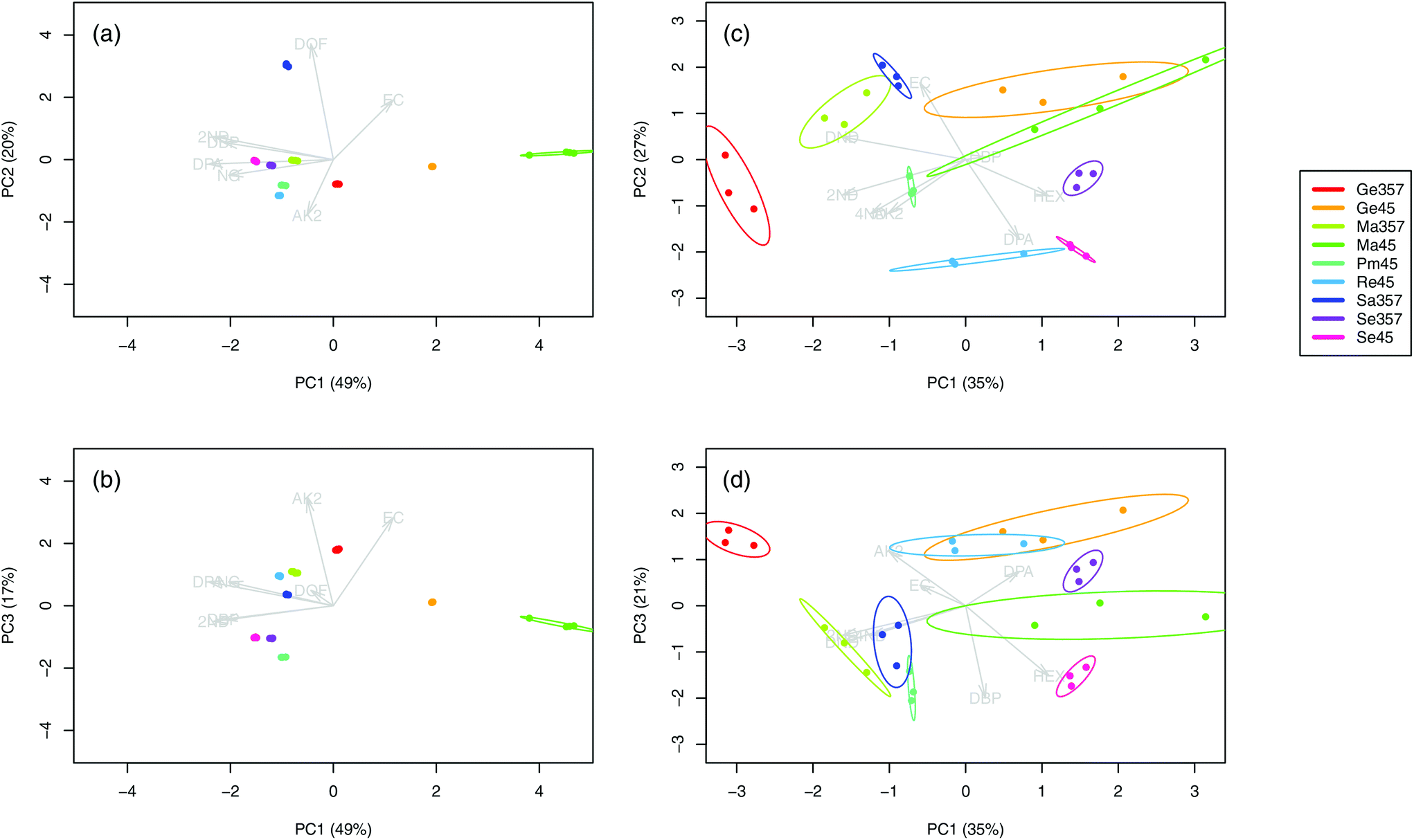 | ||
| Fig. 1 Score plots of the first three principal components for the logPA profiles (selected compounds, see Table 1) of the nine analysed SLPs (a–b, 4 replicates per SLP, n = 36) and respective OGSRs (c–d, 3 replicates per OGSR, n = 27). Arrows represent PCA loadings. | ||
For each type of ammunition, data were compared to assess the feasibility of associating OGSRs with their SLPs through simple methods. In all cases, however, significant differences were observed, which could be easily visualised in total ion chromatograms (TICs) and extracted ion chromatograms (EICs) (see example in Fig. 2). In particular, ratios of those compounds detected in both OGSRs and SLPs (i.e., DPA, 2ND, 4ND, AK2, EC and DBP) showed little consistency between pre- and post-discharge chromatograms. Their absolute peak areas also presented large inconsistencies and, most importantly, were not always well correlated (Fig. 3a). These observations were consistent with previous works on OGSR32,33 and were surely the result of a series of different factors. The discharge process itself is likely to be the most influential, given the numerous chemical reactions involved that will affect the amounts of original compound remaining and relative ratios. Further dissimilarities might be explained by the use of different sampling and extraction methods (i.e., SE and HSSE), with their specific selectivities and yields. The low-medium correlation observed between most equivalent compounds in pre- and post-discharge chromatograms highlighted complex relationships between them, which likely included non-linear and multivariate trends. This was further supported by the equally intriguing correlation patterns observed between the different compounds themselves (Fig. 3a), as well as by pre- and post-discharge similarities between general profiles. Indeed, ammunition types with very similar SLP profiles, such as Se357 and Se45, presented OGSRs with significantly different profiles, as seen in PCA score plots (Fig. 1). On the contrary, ammunition types with different SLP profiles, such as Ma357 and Sa357, presented very similar OGSR profiles. In any case, using the acquired data to directly associate OGSRs with corresponding SLPs was deemed challenging without any modelling method, as well as predicting post-discharge profiles from pre-discharge ones using univariate statistical methods.
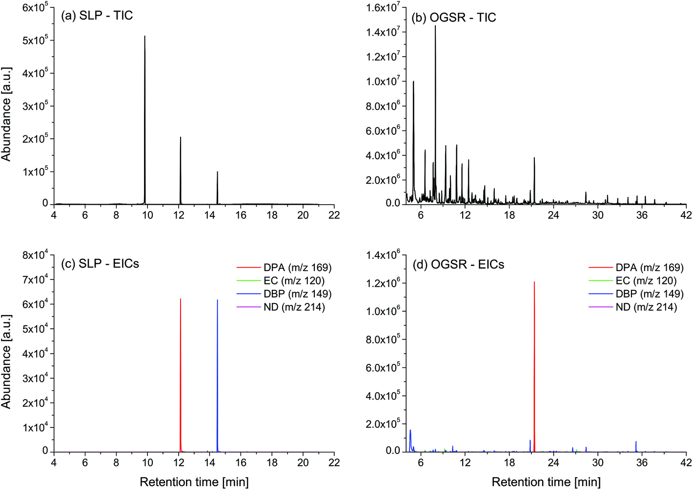 | ||
| Fig. 2 Comparison of total ion chromatograms (TICs) and overlaid extracted ion chromatograms (EICs) for selected compounds (i.e., DPA, EC, DBP, 2ND and 4ND) between a SLP analysed by SE-GC-MS and its respective OGSR analysed by HSSE-TD-GC-MS. Ammunition was a Sellier & Bellot .357 Magnum. Noteworthy are the significant differences in the ratios of the selected compounds. | ||
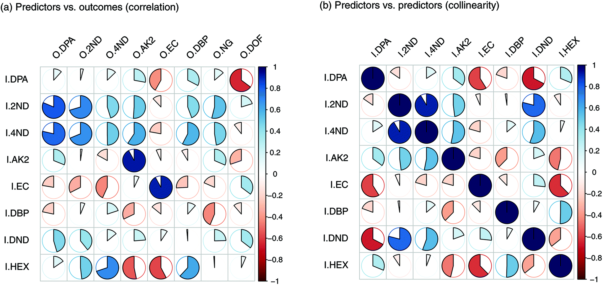 | ||
| Fig. 3 Plots of Pearson's correlation coefficients (PCCs) between (a) the input and output compounds and (b) the input compounds themselves. | ||
3.2. Predictive modelling of the single output compounds
In order to handle the aforementioned complexity and enable reliable in silico profiling, a novel modelling approach, called QPPR, was developed. The objective was to predict the measured logPAs of each of the eight compounds observed in SLP chromatograms (i.e. the “outputs” abbreviated with “O”) from those of a set of preselected compounds observed in OGSR chromatograms, taken as a group (hereafter, “inputs” abbreviated with “I”). The latter were limited to eight, which included six of the original additives observed in SLPs (i.e., DPA, 2ND, 4ND, AK2, EC and DBP) and two other molecules strictly related to their synthesis and/or degradation pathways (i.e., DND and HEX). These were mainly chosen because of their slower ageing rate and higher concentration in OGSRs compared to the other compounds, as shown in previously reported data.25 Additionally, they were either the same as, or related to, the outcome compounds. All the chosen variables are summarised in Table 1.At first, the best machine learning techniques were investigated. Fourteen multivariate regression methods, ranging from intrinsically linear methods (e.g., OLS and PLS) to inherently non-linear ones (e.g., ANN and RF), were thus tested and compared for their performances on predicting logPAs of the single output compounds for ammunition types excluded from the training database (i.e., extrapolation mode). Results are reported in Fig. 4, after tuning and optimisation of every fitted model by resampling (see also Table S4 is ESI†). An extrapolation perspective was specifically adopted at this stage, as it represents the worst-case forensic scenario. The MARS algorithm did not converge to a solution for some resampled data subsets during the training of models for OAK2 and ODOF. It was therefore excluded from further evaluation of these output compounds. For the remaining subsets, MARS, in any case, showed the highest median RMSE across all the outputs (1.628 logPA) and was thus the method providing the worst average prediction accuracies. On the contrary, RF-CART displayed the lowest median RMSE (1.233 logPA). It was followed by SVM-POL (1.259 logPA) and CR (1.261 logPA).
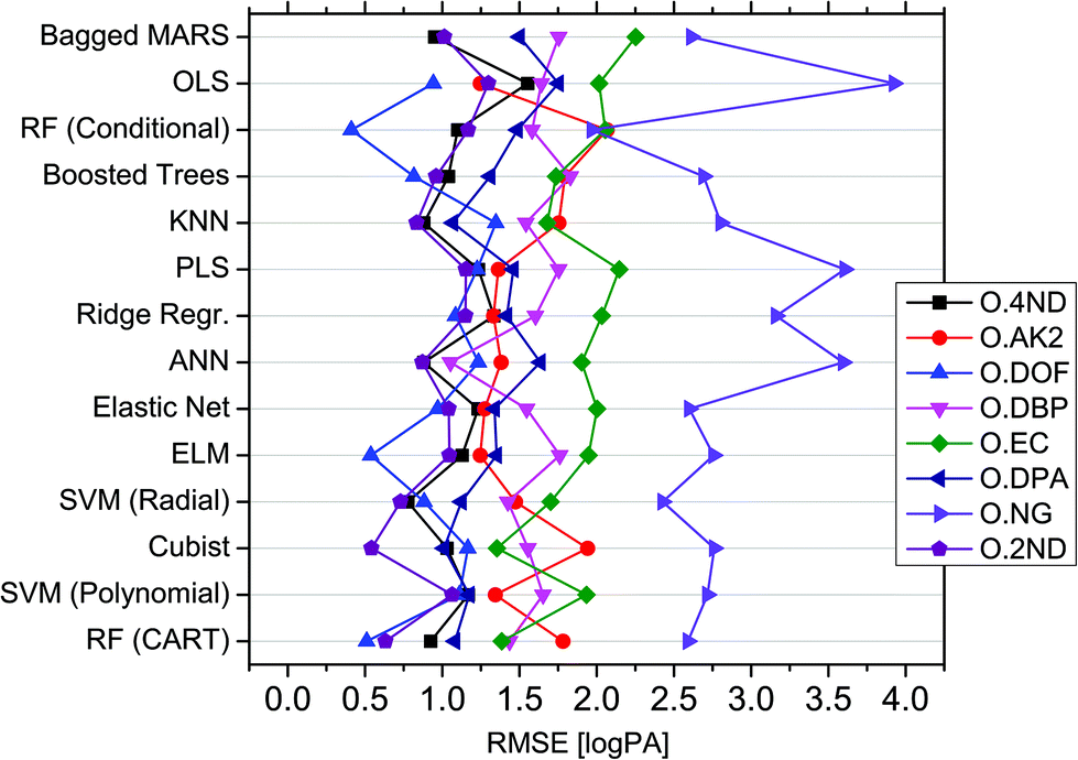 | ||
| Fig. 4 Comparison of the root-mean-square errors (RMSEs) observed on predicted logPAs for the eight output compounds (extrapolation mode), as a function of the fourteen tested regression methods. Regression methods were ranked according to their median RMSE (highest at the top; lowest at the bottom). RMSE values for the application of Bagged MARS to OAK2 and ODOF are missing because of its failure during training of respective models. | ||
On closer inspection, the performances of the different tested methods were found to actually be output-dependent (Fig. 4). For example, ANN offered significantly better performance for ODBP whilst generally ranking in the middle according to its median RMSE (1.307 logPA) across all output compounds. OLS was the method yielding the best accuracy for OAK2, despite its poor performance for the other outputs. ONG seemed the most challenging compound to be predicted, given the large RMSEs across the different regression methods. RF-CIT, however, offered significantly better performance compared to the other techniques. Cubist was the most accurate method for predicting ODPA, OEC and O2ND. Interestingly, the technique providing the best average performance (i.e., RF-CART) was not the best method for any of the outputs in particular. Correlations between the absolute errors observed after fitting using the different regression techniques were relatively low (general average around 0.65), thus supporting a low statistical dependence between them (see Fig. S3 in ESI† for further details).
Non-linear regression methods performed better, on average, on a higher number of outputs (seven vs. one; see Table S5 in ESI†). This further supported the existence of important non-linear (and multivariate) relationships between variables. As perhaps expected, for both classes of regression methods, a negative correlation between their RMSE and the mean logPAs and logPA ranges was observed across the different output compounds, meaning that the most accurate results were generally obtained on the less concentrated and less variable output compounds. The mean RMSE difference observed between linear and non-linear methods (δRMSE), however, was positively correlated with the degree of linearity of the outputs with the inputs (Fig. S4 in ESI†). As a consequence, the enhancement in performance actually depended on the observed deviation from linearity. Linear methods performed better on the outputs showing the most linear relationship with the inputs, and vice versa. Overall, all these results showed that a compound-dependent choice of techniques may be advantageous for the purpose of profile reconstruction. Best models for each output compound are reported in Table 1.
Input importance in the prediction of the eight outputs was estimated (Fig. 5). I2ND was found to be particularly important, as it explained a large amount of variability for most of the outputs, including ODPA, O2ND, O4ND, ONG and ODBP. The next most important inputs were IEC, IHEX, IDPA and IAK2. The less important ones were I4ND, IDND and IDBP. For the first two, in particular, this was most likely due of their strong collinearities with I2ND, which make them redundant and downgraded their role in regression (Fig. 3b). In any case, all input compounds showed a non-negligible impact on at least one output, supporting the usefulness of the entire set. Furthermore, all outputs were significantly influenced by more than one input, which again supported the need for a multivariate approach in QPPR modelling.
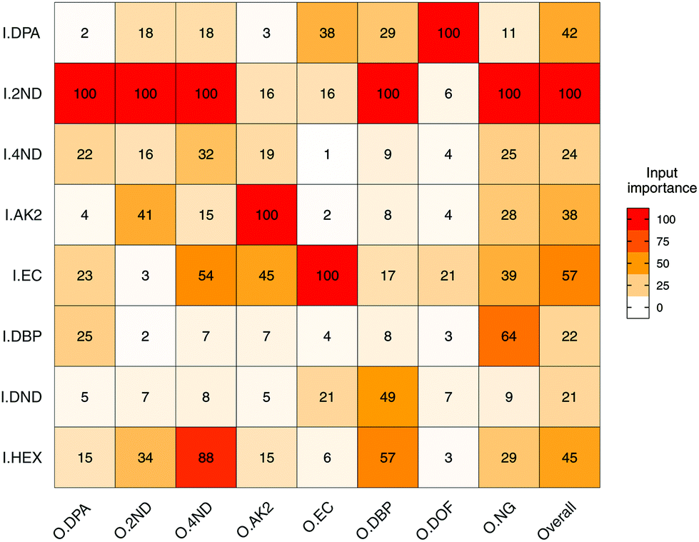 | ||
| Fig. 5 Heatmap of the mean importance (from 0 to 100%) for the eight selected input compounds (I) in the prediction of logPAs of the eight output compounds (O). Mode used was extrapolation. | ||
3.3. Selection of an optimal set of models
As for the variable performance of the tested regression methods in the prediction of the different outputs, the selection of an optimal combination of models (CoM) was deemed particularly important to guarantee both a high accuracy in profile reconstruction and increased performance regarding evidence association/discrimination. In particular, two different selection approaches were tested and compared, which were based on different criteria:- CoM1: the eight equivalent models (same regression method) that minimised the median RMSE of logPAs across all the response compounds (i.e., RF-CART);
- CoM2: the eight different models (variable regression methods) that minimised the single RMSEs of logPAs for each specific response compound (see Table 1).
Predicted SLP profiles were first compared pairwise with their respective measured profiles in order to assess similarity, which was measured through Pearson's correlation coefficient (PCC). Experiments were performed in both extrapolation and interpolation modes, in order to test for accuracy differences in case of inclusion of the ammunition of interest in the training library.
Overall, CoM2 led to highly accurate predicted profiles in both extrapolation and interpolation modes on average (Fig. 6). Indeed, a median PCC value of 0.908 and interquartile range (IQR) from 0.874 to 0.937 were observed after within-source comparisons between extrapolated and measured profiles, while a median PCC value of 0.986 and IQR from 0.926 to 0.994 were observed between interpolated and measured profiles. Concerning CoM1, the degree of similarity observed was more dependent on the exhaustiveness of the training dataset. In fact, despite the results obtained on interpolated profiles being very similar to CoM2 (distribution of PCCs with a median value of 0.982 and IQR from 0.965 to 0.993), those observed in extrapolation mode had significantly lower PCCs. A median PCC value of 0.839 and IQR from 0.711 to 0.918 were observed, which proved that CoM1 less accurately predicted profiles than CoM2, in those cases where the ammunition type of interest was not included in the training dataset. Similar results were also observed if the eight RF-CART models in CoM1 were substituted with the corresponding SVM-POL or CR ones, which were the next best predictive regression methods (data not shown).
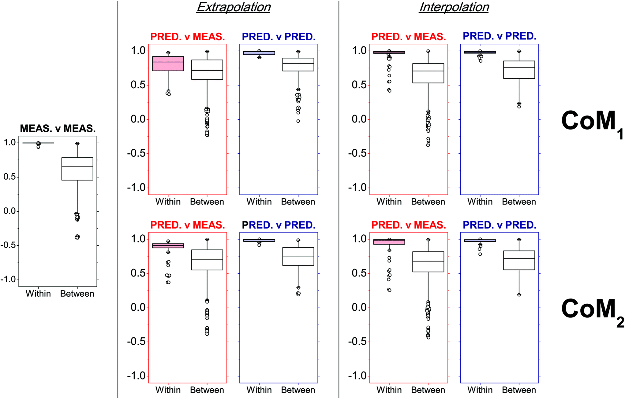 | ||
| Fig. 6 Within- and between-ammunition distributions of Pearson's correlation coefficients (PCCs) observed after comparison of SLP profiles in a number of different situations (measured–measured, predicted–measured, predicted–predicted), as a function of the tested combinations of models (CoMs). Within-ammunition PCC distributions observed in predicted–measured comparisons (i.e., red boxplots) were particularly used to assess prediction accuracies. The number of observed PCCs (n) included in each boxplot is reported in Table S8 in ESI.† | ||
Between-source comparisons between predicted and measured SLP profiles were performed. As perhaps expected, observed PCC values were, on average, lower than those obtained from within-source comparisons for both CoMs (Fig. 6). Furthermore, IQRs of between-source distributions did not overlap with those of the respective within-source distributions for most of the situations. This was promising for the purpose of correctly associating questioned GSRs with their corresponding ammunition. Receiver operating characteristics (ROC) analysis was used to assess this potential, using both CoMs. Results are summarised in Fig. 7. Almost identical results were obtained on interpolated profiles, with areas under curve (AUCs) of 0.916 and 0.894 for CoM1 and CoM2, respectively. In extrapolation mode, on the contrary, the lower accuracy in profile reconstruction previously observed with CoM1 led to big differences in the association performance compared to that observed with CoM2. Indeed, AUCs of 0.633 and 0.824 were observed in this case for CoM1 and CoM2, respectively. Therefore, overall, CoM2 allowed both superior accuracy in profile reconstruction and enhanced discrimination of within- and between-source distributions of PCCs. This was selected as optimal. As a result, the use of a unique machine learning technique to predict all the single outputs was not deemed an advantageous strategy, at least on this dataset: a multimodal approach is preferable. For the sake of illustration, Fig. 8 shows examples of the comparison between measured profiles and those predicted with CoM2.
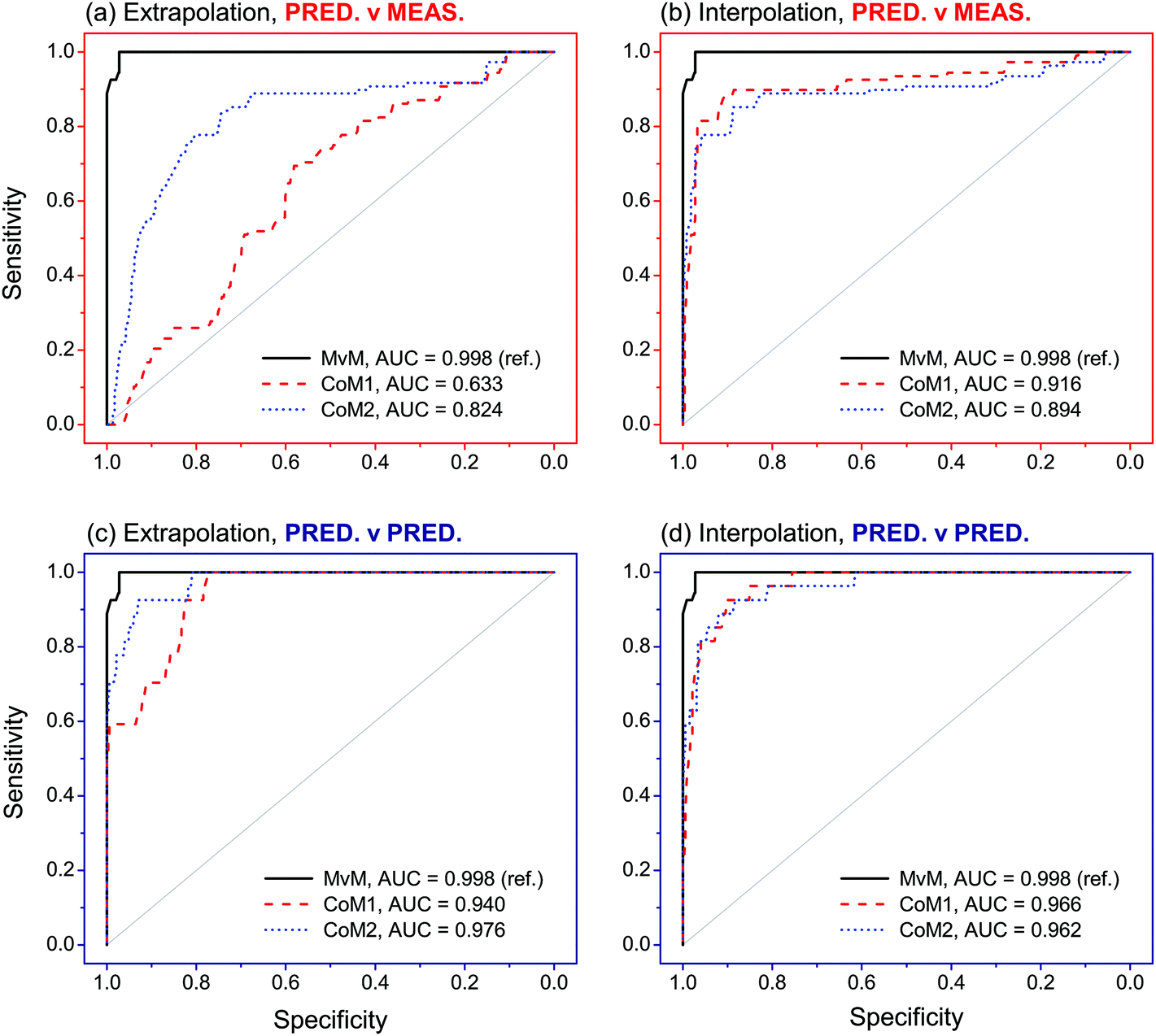 | ||
| Fig. 7 Receiver operating characteristic (ROC) curves observed after analysis of PCCs obtained in the comparisons between predicted–measured and predicted–predicted profiles, as a function of the tested combinations of models (CoMs). The closer the ROC curves are to the upper left corner, the higher the overall association performances. Measured–measured (MvM) comparisons were used as reference for validation. Areas under the curve (AUCs) are also reported (maximum allowed value is 1). The number of PCCs (n) included in each ROC curve is reported in Table S8 in ESI.† | ||
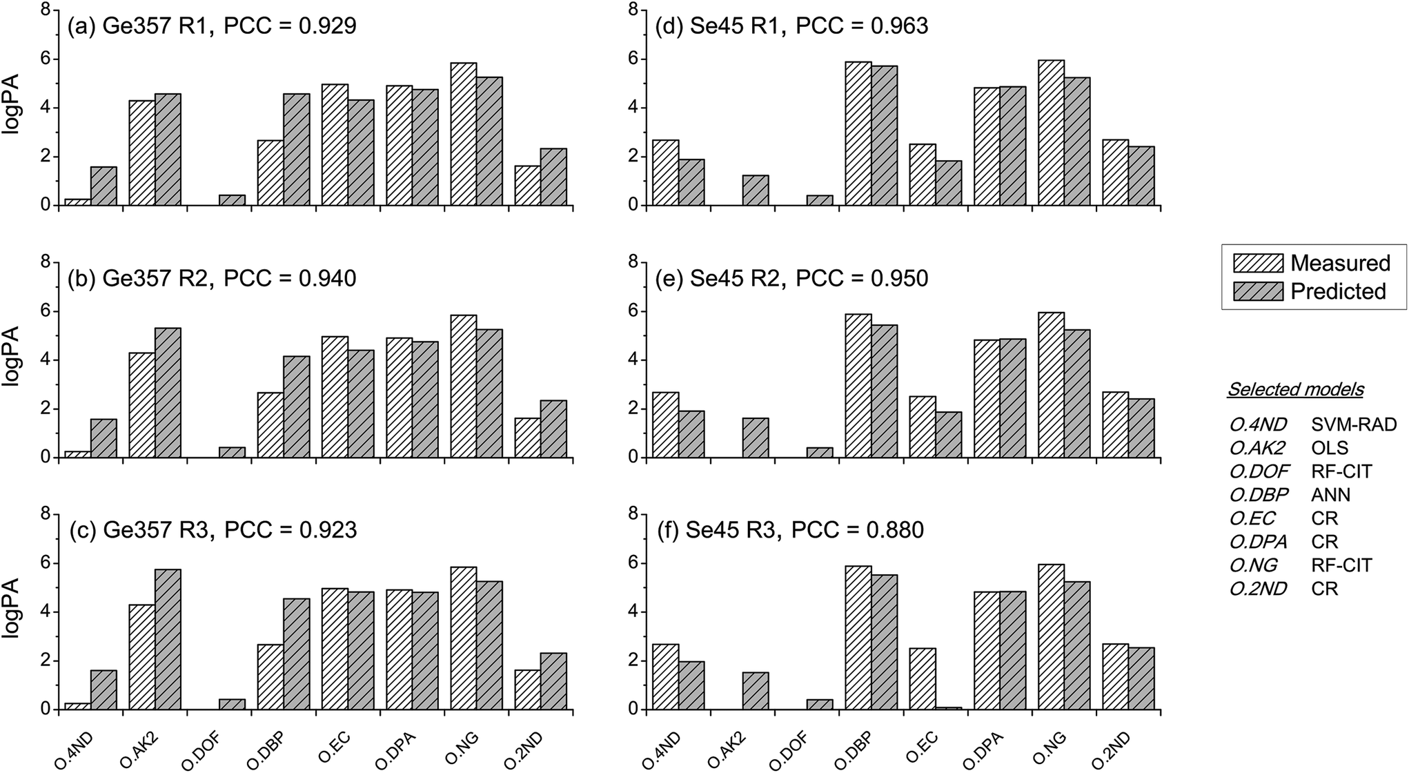 | ||
| Fig. 8 Comparison between measured and predicted SLP profiles for two ammunition types: Magtech .357 Magnum and Sellier & Bellot .45 ACP. For each ammunition, predicted profiles were obtained by assembling logPAs returned by the optimal combination of models (i.e., CoM2, reported at right side of the image) for three different replicate OGSR analyses (extrapolation mode). | ||
Even using the optimal model combination, a few outliers were still observed, especially in within-source distributions of PCCs for the comparison of predicted–measured profiles. Upon closer inspection, it could be noted that these all belonged to the Ma45 ammunition (Fig. 6; see also Table S6 in ESI†), which was not surprising. Being a single-base propellant, measured SLP profiles displayed particularly rare features compared to those of the other SLPs (see PCA plots in Fig. 1a and b), making them particularly hard to be predicted, especially in extrapolation mode. Results obtained in interpolation mode generally showed a better accuracy. This proved the ability of the approach to learn and further improve itself from additional data included in the training dataset, as well as the added value of working with exhaustive training datasets.
3.4. Evaluation of overall association performances
Evaluation of association performances was extended to other scenarios. In particular, pairwise comparisons between predicted–predicted profiles were performed, in addition to those previously performed between predicted-measures profiles. From a forensic point of view, these correspond to the cases where association is attempted between GSR–GSR and GSR–ammunition, respectively. Comparisons between measured–measured profiles (i.e., association between ammunition–ammunition) were also performed in order to serve as reference and to further validate the approach.Comparisons between measured–measured profiles showed excellent results (Fig. 7). Indeed, an AUC of 0.998 was observed after ROC analysis, which was really close to the maximum value of 1 and thus showed an almost perfect ability to correctly predict whether two samples come from the same or different sources. Comparisons between predicted–predicted profiles achieved largely comparable results in both extrapolation and interpolation modes. With the optimal set of models (i.e., CoM2), in particular, AUCs of 0.940 and 0.966 were observed, respectively. Particular noteworthy was that no significant differences between association performances were observed between the different tested sets of models on both extrapolated and interpolated profiles. Comparisons between predicted–measured profiles were slightly less performant and, again, more dependent on the exhaustiveness of the training dataset. Indeed, AUCs of 0.824 and 0.894 were observed with CoM2 on extrapolated and interpolated profiles, respectively, as reported in the previous section. These latter values, however, are still high and close to those observed in the previous scenarios.
Considering the similar results observed after ROC analysis between the comparisons of measured–measured and predicted–predicted profiles, the final developed and optimised QPPR modelling approach proved to be particularly efficient at matching predicted SLP profiles between them and also associating samples in GSR–GSR scenarios. It, furthermore, showed a remarkable robustness to model selection in this specific application, as supported by the high consistency between the two tested CoMs. All these observations were, nonetheless, perhaps expected, considering that the application of the same CoM to different OGSR samples released from the same ammunition type is prone to naturally converge to the same profiles. This leads to high PCCs independent from the actual similarity of the predicted profiles with those experimentally measured on the original SLP, which is an important advantage in view of applications in which GSR–GSR associations are of interest. Results are promising but further tests are necessary to investigate if GSR–GSR comparisons between residues recovered from different locations would also benefit from use of such an approach.
Comparison of predicted–measured profiles proved to be more challenging, as shown by the higher sensitivity of the results to the CoM and slightly lower association performances compared to both measured–measured and predicted–predicted comparisons. This was due to the presence of systematic prediction errors in SLP profiles after QPPR modelling. As for this, the choice of an optimal CoM was shown to be extremely critical, but good association performances were obtained using a multimodal approach (Fig. 7 and 8). These were close to those observed in the other comparison scenarios and thus strongly supported the possibility of using the developed QPPR approach for evidence association in GSR–ammunition scenarios.
4. Conclusion
A novel in silico profiling approach, known as quantitative profile–profile relationship (QPPR) modelling, was successfully used to predict profiles of smokeless powders (SLPs) from those of the respective organic GSR (OGSRs) in spent cases. Promising results were observed through an adequate optimisation of the modelling procedure to include a multimodal combination of different machine learning techniques. ROC analysis was used to assess association performances and showed a remarkable potential to correctly associate OGSRs with the respective unexploded SLPs. To our knowledge, this work represents the first time that a quantitative approach has successfully been applied to make an association in a GSR–ammunition scenario. Very promising results were also observed for association of samples in GSR–GSR scenarios.The developed approach represents a significant and valuable improvement compared to those currently available for evidence association in GSR analysis. It particularly showed increased association capability, enhanced flexibility across forensic scenarios, less reliance on case-related reference ammunition and a reduced requirement for supplementary analyses. Indeed, QPPR can enable association of samples through the use of general statistical models that can be applied to a large number of different cases. For example, this can be used as a screening technique, in order to focus further actual analyses on pertinent reference material only, thus minimising consumption of materials, time and money. Potential for further developments is promising. QPPR modelling, in particular, could be extended for application to data acquired with other analytical methods, such as OGSR analysed by liquid chromatography. Adaptation to pGSR seems also feasible, through exploitation of elemental profiles of particles and/or distribution of particle types. The successful development of specific QPPR models for all these types of residues would potentially allow association of GSR samples deposited on different surfaces. It could also unlock wholly new possibilities in the field, such as the comparison of GSRs recovered from different crime scenes, in order to link events and introduce new “profiling” and “intelligence-led” perspectives.44 The benefits are countless and may even extend to other fields in analytical sciences that routinely encounter mutable chemical traces, such as, for example, the analysis of improvised explosive devices, arson accelerants, toxicological samples and environmental contaminants/pollutants.
Conflicts of interest
There are no conflicts to declare.Acknowledgements
This work has been kindly supported by the Swiss National Science Foundation (Grant No. P2LAP1_164912). The authors would like to thank Rachel Irlam (King's College London, UK) for proof-reading the document.References
- K. Inman and N. Rudin, Principles and practices of criminalistics, CRC Press, Boca Raton, USA, 2001 Search PubMed.
- M. G. Haag and L. C. Haag, Shooting incident reconstruction, Academic Press, San Diego, USA, 2nd edn, 2011 Search PubMed.
- B. J. Heard, Handbook of firearms and ballistics, John Wiley & Sons, Hoboken, USA, 2nd edn, 2008 Search PubMed.
- J. S. Wallace, Chemical analysis of firearms, ammunition, and gunshot residue, CRC Press, Boca Raton, USA, 2008 Search PubMed.
- F. S. Romolo and P. Margot, Forensic Sci. Int., 2001, 119, 195–211 CrossRef.
- O. Dalby, D. Butler and J. W. Birkett, J. Forensic Sci., 2010, 55, 924–943 CrossRef PubMed.
- H.-H. Meng and B. Caddy, J. Forensic Sci., 1997, 42, 553–570 CAS.
- L. S. Blakey, G. P. Sharples, K. Chana and J. W. Birkett, J. Forensic Sci., 2018, 63, 9–19 CrossRef PubMed.
- M. Maitre, K. P. Kirkbride, M. Horder, C. Roux and A. Beavis, Forensic Sci. Int., 2017, 270, 1–11 CrossRef CAS PubMed.
- K.-M. Pun and A. Gallusser, Forensic Sci. Int., 2008, 175, 179–185 CrossRef CAS PubMed.
- V. R. Matricardi and J. W. Kilty, J. Forensic Sci., 1977, 22, 725–738 CAS.
- G. M. Wolten, R. S. Nesbitt, A. R. Calloway, G. L. Loper and P. F. Jones, J. Forensic Sci., 1979, 24, 409–422 CAS.
- J. Lebiedzik and D. L. Johnson, J. Forensic Sci., 2000, 45, 83–92 CAS.
- H.-H. Meng and H.-C. Lee, Forensic Sci. J., 2007, 6, 39–54 Search PubMed.
- S. Benito, Z. Abrego, A. Sanchez, N. Unceta, M. A. Goicolea and R. J. Barrio, Forensic Sci. Int., 2015, 146, 79–85 CrossRef PubMed.
- J. Andrasko, J. Forensic Sci., 1992, 37, 1030–1047 CAS.
- M. Morelato, A. Beavis, A. Ogle, P. Doble, P. Kirkbride and C. Roux, Forensic Sci. Int., 2012, 217, 101–106 CrossRef CAS PubMed.
- F. S. Romolo, A. Stamouli, M. Romeo, M. Cook, S. Orsenigo and M. Donghi, Forensic Chem., 2017, 4, 51–60 CrossRef CAS.
- Z. Brozek-Mucha and A. Jankowicz, Forensic Sci. Int., 2001, 123, 39–47 CrossRef CAS PubMed.
- Z. Brozek-Mucha, G. Zadora and F. Dane, Sci. Justice, 2003, 43, 229–235 CrossRef CAS PubMed.
- Z. Brozek-Mucha and G. Zadora, Forensic Sci. Int., 2003, 135, 97–104 CrossRef CAS PubMed.
- S. Steffen, M. Otto, L. Niewoehner, M. Barth, Z. Brozek-Mucha, J. Biegstraaten and R. Horvath, Spectrochim. Acta, Part B, 2007, 62, 1028–1036 CrossRef.
- M. R. Rijnders, A. Stamouli and A. Bolck, J. Forensic Sci., 2010, 55, 616–623 CrossRef PubMed.
- M. E. Christopher, J.-W. Warmenhoeven, F. S. Romolo, M. Donghi, R. P. Webb, C. Jeynes, N. I. Ward, K. J. Kirby and J. A. Bailey, Analyst, 2013, 138, 4649–4655 RSC.
- M. Gallidabino, F. S. Romolo and C. Weyermann, Anal. Bioanal. Chem., 2015, 407, 7123–7134 CrossRef CAS PubMed.
- J. Lebiedzik and D. L. Johnson, J. Forensic Sci., 2002, 47, 483–493 CAS.
- H. Wrobel, J. J. Millar and M. Kijek, J. Forensic Sci., 1998, 43, 324–328 CAS.
- D.-M. K. Dennis, M. R. Williams and M. E. Sigman, Forensic Chem., 2017, 3, 41–51 CrossRef CAS.
- M. R. Reardon, W. A. MacCrehan and W. F. Rowe, J. Forensic Sci., 2000, 45, 1232–1238 CAS.
- W. A. MacCrehan, M. R. Reardon and D. L. Duewer, J. Forensic Sci., 2002, 47, 260–266 CAS.
- Z. Brozek-Mucha, X-Ray Spectrom., 2007, 36, 398–407 CrossRef CAS.
- K. L. Reese, A. D. Jones and R. W. Smith, Forensic Sci. Int., 2017, 272, 16–27 CrossRef CAS PubMed.
- A.-L. Gassner and C. Weyermann, Forensic Sci. Int., 2016, 264, 47–55 CrossRef CAS PubMed.
- A. Duarte, L. M. Silva, C. T. De Souza, E. M. Stori, L. A. B. Niekraszewicz, L. Amaral and J. F. Dias, Forensic Chem., 2018, 7, 94–102 CrossRef CAS.
- M. Gallidabino, A. Biedermann and F. Taroni, J. Forensic Sci., 2015, 60, 539–541 CrossRef PubMed.
- M. I. Jordan and T. M. Mitchell, Science, 2015, 349, 255–260 CrossRef CAS PubMed.
- Y. LeCun, Y. Bengio and G. Hinton, Nature, 2015, 521, 436–444 CrossRef CAS PubMed.
- C. Nantasenamat, C. Isarankura-Na-Ayudhya, T. Naenna and V. Prachayasittikul, EXCLI J., 2009, 8, 74–88 Search PubMed.
- C. Nantasenamat, C. Isarankura-Na-Ayudhya and V. Prachayasittikul, Expert Opin. Drug Discovery, 2010, 5, 633–654 CrossRef CAS PubMed.
- M. Kuhn and K. Johnson, Applied predictive modeling, Springer, New York, USA, 2013 Search PubMed.
- M. Gallidabino, F. S. Romolo, K. Bylenga and C. Weyermann, Anal. Chem., 2014, 86, 4471–4478 CrossRef CAS PubMed.
- T. Fawcett, Pattern Recognit. Lett., 2006, 27, 861–874 CrossRef.
- J. Andrasko, T. Norberg and S. Stahling, J. Forensic Sci., 1998, 43, 1005–1015 Search PubMed.
- M. Morelato, A. Beavis, M. Tahtouh, O. Ribaux, K. P. Kirkbride and C. Roux, Forensic Sci. Int., 2013, 226, 1–9 CrossRef PubMed.
Footnote |
| † Electronic supplementary information (ESI) available. See DOI: 10.1039/c8an01841c |
| This journal is © The Royal Society of Chemistry 2019 |