Thermo-economic analysis and multi-objective optimisation of lignocellulosic biomass conversion to Fischer–Tropsch fuels

Abstract

This paper addresses the techno-economic evaluation and optimisation of processes converting lignocellulosic biomass into liquid fuels, through the development of a suitable framework and the modelling and design of Biomass to Liquids (BTL) processes. In particular, the focus is on the production of drop-in fuels through gasification and Fischer–Tropsch (FT) synthesis. Several conversion technologies are presented and evaluated in the literature, but the comparison of different options is hazardous because of the different assumptions and methodologies adopted in each study. A systematic and consistent approach is therefore developed to explore the trade-offs of alternative process configurations and of the operating conditions. The comparison presented in this study explores the trade-offs of different technological options in terms of competing economic and thermodynamic objectives. Results show that for 200 MW_th biomass input plant capacities, production costs are in the range of 1.0–1.4 € l⁻¹ for technologies producing up to about 0.5 kJ_FT kJ_th⁻¹ and close to being neutral in terms of electricity balance. For technologies using electrolysis the conversion can increase to 0.8 kJ_FT kJ_th⁻¹ with production costs of 1.8 € l⁻¹. The electricity storage capacity, in this case, is of 0.5 kJ_e kJ_FT⁻¹, corresponding to a net electricity requirement of about 0.4 kJ_e kJ_th⁻¹.

---

1 Introduction

The growing interest in the use of biomass for the production of liquid fuels is driven by the potential to (i) reduce Greenhouse Gas (GHG) emissions by displacing the use of fossil-derived fuels, (ii) improve energy security by reducing oil imports for the transport sector, (iii) contribute to rural communities' development by supporting the agricultural industry and (iv) convert a low-cost low energy density material, such as organic waste, into a crude oil equivalent product.

Biomass today supplies slightly over 10% of the world's primary energy demand, with 53.48 EJ per year (53.48 10⁹ GJ) in 2011.¹ Estimates for long-term sustainable potential vary widely from 100 to 400 EJ per year in 2050, the main uncertainties being land availability and yield levels in energy crop production, but also the availability of forest wood and of residues from agriculture and forestry.²

According to the International Energy Agency (IEA) the transportation sector accounts for 19% of global energy use and about 23% of energy-related CO₂ equivalent emissions. Given the current trends, transport energy use and CO₂ emissions are projected to increase by 50% by 2030.^3,4 However, the United Nations Intergovernmental Panel on Climate Change (IPCC), suggests that at least a 50% reduction in global CO₂ emissions (compared to 2000 levels) is to be achieved by 2050 to limit the long-term global average temperature rise between 2.0 °C and 2.4 °C.⁵ In this context, the IEA proposes the BLUE map scenario ‘examining the least-cost means of achieving that goal through the deployment of existing and new low-carbon technologies’⁵ where second-generation biofuels contribute to 3% of the cumulative CO₂ emissions reduction.

Second-generation biofuels rely on lignocellulosic biomass feedstock which may include by-products (cereal straw, sugar cane bagasse, forest residues), wastes (organic components of municipal solid wastes, wood processing waste) and dedicated feedstock (purpose-grown vegetative grasses, short rotation forests and other energy crops). They should not enter in direct competition with the production of food and fodder, tackling one of the drawbacks of first generation biofuels. Some concerns remain in terms of GHG emissions related to land use change and soil degradation when removing organic matter from the land, which may affect nutrient content.⁶ The rational use of the biomass resource remains therefore of fundamental importance for second-generation fuels to be sustainable.

The two main conversion pathways for second-generation biofuels are biochemical and thermochemical conversion processes. Biochemical conversion consists in the enzymatic or chemical hydrolysis of the cellulose in biomass into sugars before fermentation to alcohols. Thermochemical conversion consists in the high-temperature thermal gasification of biomass to produce a synthesis gas rich in H₂ and CO that can be converted in transport fuels. The main steps in the process chain are feed preparation, gasification, gas cleaning and synthesis. Each of these steps can be performed with different technologies. For example, the gasifier itself, can be a fluidised bed or an entrained flow reactor.

The abundant literature on second-generation biofuels through thermochemical‡ shows the important interest for this biomass conversion pathway, from both governments, universities and the research community.

An overview and summary of the techno-economic evaluations carried out since 2002 is presented in the studies by Haarlemmer et al.^14,15 These studies present the total investment cost and production cost determined in the literature and normalised, as far as possible, to the same basis (in terms of reference year, 2011, and input capacity, 400 MW_th). The studies analysed in the literature, concern the evaluation of different technological options and process configurations, but the dispersion of the results makes drawing conclusions regarding their trade-offs very difficult. This is due to the different economic and modelling assumptions considered in each study. In particular, the investment costs of BTL processes are unavoidably affected by large uncertainties as commercial plants have yet to be built. The techno-economic studies on BTL conversion can only be considered prospective at this stage. Nevertheless, the thermochemical pathway is gaining momentum and many demonstration and pilot plants are being built, especially in Europe and North America, but also China and India.

The thermochemical conversion of biomass represents a complex system characterised by non-linear relationships and multiple interactions between the steps of the process, which in turn affect the overall performance. The conceptual design of such processes requires the development of adequate models for the representation of the conversion processes, heat integration to optimise heat recovery, and optimisation to select the best designs. Several authors have addressed this issue in the context of biomass conversion processes, using different methodologies. A detailed comparison of the methodologies goes beyond the scope of this study, but the most relevant ones are briefly summarised in Table 1.

Table 1 Main optimisation strategies applied to biomass conversion processes in the literature

Main literature	Floudas et al.^16–19	Grossmann et al.^20–22	Maréchal et al.^23–27
Optimisation	Mix Integer Non-Linear Programming (MINLP) with non-convex functions. Rigorous deterministic global optimisation approach with branch-and-bound global optimisation algorithm	MINLP using shortcut models consisting of mass and energy balances. Problem decomposed into NLP problems, implemented in GAMS	MINLP problem decoupled in a master optimisation problem and a slave problem. Heuristic multi-objective optimisation using an evolutionary algorithm
Objective	Minimum production cost (optimal topology, scenario type investigation)	Simplified production cost (income from products and expenditures for energy and utilities) or energy input	Multi-objective: investment cost, efficiency, environmental performance, etc.
Solution	Guaranteed to be within a small percentage of the best possible value	—	The optimisation is ended after a large number of iterations
Heat integration	Simultaneous	Heat exchanger network design (SYNHEAT)^28 for the optimal solution	Heat integration formulated as a MILP problem,^29 simplified estimate of the HEN cost as part of the slave problem
Operating conditions	Fixed points (i.e. gasifier temperature)	Continuous variables, part of the decision variables	Continuous and integer variables, part of the decision variables
Feedstock	Biomass, coal, natural gas	Biomass	Biomass, coal
Products	FT, methanol, methanol to gasoline, methanol to olefines	Hydrogen. FT, ethanol	Synthetic Natural Gas (SNG), hydrogen

---

The first two methodologies presented in Table 1 have the advantage of using rigorous optimisation techniques, but evaluate a single objective. The methodology reported in the third column of Table 1, proposed by Maréchal et al.^23–27 uses a master-slave optimisation approach and uses heuristic multi-objectives optimisation techniques at the master level. It allows multiple objectives as well as both continuous and integer variables to be considered. This methodology is at the basis of the work carried out in this study.

In the context of BTL conversion routes, beyond the thermo-economic evaluation by Tock et al.,³⁰ such a holistic approach has not yet been applied. This study proposes a comprehensive process integration approach in which design options, technological alternatives, and operating conditions, that could be implemented in a BTL plant, are systematically and thoroughly compared on a consistent basis.

The main objective of this work is therefore to propose a framework for the analysis of BTL conversion routes, which allows a large number of process chains to be systematically generated and evaluated by selecting the unit operations belonging to a superstructure. Such framework, described in Section 2 allows the synergies between the process steps to be systematically exploited through process integration and the effect of process variable to be taken into account through multi-objective optimisation.

The second objective is to carry out a detailed analysis of the alternative process designs to evaluate the effect of different technological options on performance and for a through comparison with previous literature results. The definition and the results of this analysis are presented and discussed in Section 3.

2 Methodology

The methodology adopted in this study is based on the previous work by Bolliger³¹ and Maréchal et al.^29,32,33 Bolliger³¹ developed a framework for the synthesis of industrial energy systems through multi-objective optimisation, based on the separation of the unit models from the data required for their heat and mass integration. Maréchal et al.^29,32,33 formulated the integration of the optimal utility system as a Mix Integer Linear Programming (MILP) problem, including the combined production of heat and power.

The resolution strategy adopted in this study for the design and evaluation of BTL conversion routes is schematically represented in Fig. 1.

Fig. 1 Process system design methodology.

The first step is the conceptual design of the superstructure, presented in Section 2.1, representing the unit operations and the possible process options to be investigated. The unit operations correspond to single alternative technologies which may be selected to evaluate different process chains. The superstructure approach allows, therefore, for a large number of configurations to be extracted and evaluated.

For each unit operation, a thermochemical model is developed for the computation of the energy and mass balances, as well as the excess and required heat and corresponding temperature levels. The models are developed using the flowsheeting software Vali™ by Belsim³⁴ and summarised in the ESI.†

These models are coupled with the process integration optimisation algorithm, which closes the energy balance by maximising the production of fuel and by optimising the heat integration of the process, the co-production of power. The process integration model is formulated as a MILP optimisation problem to calculate the flow-rates corresponding to each unit (or sub-system), such as the process units, the heat recovery units, the utilities (hot and cold). The heat requirement (hot utility) is provided by the combustion of the off-gases from the process. If this is not sufficient, selected process streams can be used as fuel to close the balance, reducing the overall production. The cooling requirement (cold utility) is provided by conventional cooling by river water. The detailed formulation of the process integration optimisation problem is described elsewhere^24,29,32,33 and the general assumption can be found in the ESI.†

Once the process is completely defined, the performance evaluation can be carried out according to thermodynamic, environmental and economic criteria described in Section 2.2.

The results of the performance evaluation can then be used as objectives in the frame of a Multi-Objective Optimisation (MOO). The MOO is carried out using the evolutionary algorithm developed by Molyneaux et al.^35,36 Given the decision variables, the optimal solutions in terms of conflictive objectives can therefore be obtained. The integer variables represent binary type choices, for example, the type of technology, the optional inclusion of a co-generation unit and/or a heat pump, or process configurations, such as the activation of optional interconnection between units. The continuous variables represent the operating conditions (for example temperatures, pressures, recycling fractions etc.) of the process and may regard both the thermochemical models of the unit operations and the energy recovery systems belonging to the process integration model. The resolution is set up as a slave sub-problem (the thermochemical, the energy integration, the economic models) and a master problem (the MOO), as displayed in Fig. 1.

2.1 Process design

The ideal conversion of biomass into liquid FT fuels can be summarised by eqn (1).

The stoichiometry of this general ideal reaction shows that biomass lacks hydrogen and has oxygen in excess with respect to the FT fuel. Oxygen is removed in the form of water and carbon dioxide, and only part of the biogenic carbon is converted into the final fuel. The overall process is shown to be slightly exothermic.

As an alternative, it is possible to imagine adding enough hydrogen to the system (in the form of water) and removing oxygen (in the form of molecular oxygen) so as to convert all the carbon in biomass to carbon in the final FT fuel. The ideal conversion can be represented by eqn (2). In this case the reaction is endothermic, indicating that energy will be needed to realise the operation.

However, in order to achieve such a high conversion, pure O₂ would need to be removed, not only from the added water, but also from the original biomass.

In practice, BTL processes, begin with a pre-treatment section, where biomass is generally dried, reduced in size and optionally torrefied and/or transformed into pellets, in order to make it suitable for the following steps. Pre-treatment can be carried out on the same site as the rest of the process or in a different site, close to where biomass is harvested/collected, in order to reduce transportation costs. Gasification transforms biomass into a raw synthesis gas, mainly composed of CO, H₂, CO₂ and other minor gases and contaminants. This gas is cooled, cleaned, and its composition is adjusted in the gas conditioning section, so it satisfies the specifications required for the synthesis. In the synthesis section, the clean synthesis gas is transformed into the final liquid fuel.

The literature describes a large number of possible options and technologies that could be implemented in BTL conversion plants. In order to limit the dimensions of the problem, the first step of the analysis is the layout of a superstructure encompassing a subset of technologies, hereafter referred to as unit operations and process options of interest. This selection is represented in Fig. 2. This figure also shows the optional recycles, material flows and the heat recovery in the steam network for the co-production of electricity.

Fig. 2 Superstructure representing the process design of the technologies of interest for BTL conversion. The technologies retained for the final evaluation and optimisation in this study are displayed in black font. The ones suggested for future evaluation in grey font.

The possibility of adding hydrogen to the system, shown in eqn (2) with respect to eqn (1), is represented in the process design by using the High-Temperature Electrolysis (HTE) as an alternative to the Water Gas Shift (WGS) unit operation.

The system boundaries are represented in Fig. 2 by the dashed line. The material and energy flows crossing these boundaries from and to the ‘environment’ are:

• Biomass: delivered to the BTL plant or the pretreatment facility in the form of wood-chips;

• Fuel: the final product, a drop-in fuel§ which can be used in the current infrastructure;

• Electricity: which is bought/sold from/to the grid;

• Carbon dioxide: which can be an emission from combustion (diluted with N₂) or ‘storage ready’ from the Acid Gas Removal (AGR) process;

• Water: considered available from the environment.

• Air: considered available from the environment;

The upstream processes, such as electricity production, and with regard to biomass: harvesting, chipping, transportation from the harvesting grounds to a collection site, are not directly included in the superstructure. Similarly CO₂ sequestration and the final use of the fuel are not part of the analysis.

The process unit operations retained and evaluated in this study, represented in black font in Fig. 2, stems primarily from the literature survey of promising process options for BTL conversion. The selection is of course also based on the possibility to accurately model them and represent the trade-offs between competing options in the context of this study. The ‘reduced’ superstructure, including only the technologies evaluated in this study, is inherently limited, but the approach allows the coherent comparison and optimisation of a large number of options and always leaves the possibility for the addition of new ones. The unit operations represented with the grey font are suggested for future evaluation.

2.2 Performance evaluation

The performance evaluation is carried out calculating several indicators representing the thermodynamic, economic and environmental performance. The indicators can be used as criteria, to evaluate and compare different processes, or as the objective functions, for the MOO. The indicators considered in the present study are described hereafter.

2.2.1 Thermodynamic performance. The thermodynamic performance is evaluated by considering several definitions of efficiency (η), which are used in this study to represent the different relative importance of resources and products.

These definitions are reported in eqn (3)–(5).

the superscripts − and + refer respectively to net produced (output) and consumed (input) services, and ΔĖ = |Ė⁻ − Ė⁺|.

Eqn (3) represents the first thermodynamic principle of energy efficiency, for which electricity, biomass and FT fuel are evaluated on an energy basis (the Lower Heating Value (LHV) for biomass and the FT fuel). Either the net electric power input (ΔĖ⁺) or output (ΔĖ⁻) of the process is considered, since only the overall balance is of interest.

Eqn (4) represents chemical conversion efficiency and takes into account the fraction of the heating value of the final fuel with respect to that of the biomass input.

Eqn (5), represents the equivalent conversion efficiency. The term represents the fuel equivalent of the electricity produced or consumed by the process. ΔĖ* is positive if it represents a net output and negative otherwise. The value of η_substitution therefore depends on the type of technology considered as a reference. If an internal combustion engine is used to generate electricity its efficiency is about 33%.³⁷ A flexible fuel gas turbine operating in combined cycle has an electric efficiency of about 50%.³⁸ The highest efficiency for this type of cycle, operating on natural gas, is about 60% (60.75%).³⁹ The value considered for η_substitution represents the trade-off assumed between the production of electricity and fuel. A lower value corresponds to a higher relative weight of electricity in the calculation of η_{en_eq}. When this indicator is set as an objective of the optimisation, the choice η_substitution may affect the optimal solutions, depending on the type of process considered. The value retained for η_substitution, is 60%. This value allows to take into consideration that the FT fuel is the main product of the BTL process, while assigning technical relevance to the net electricity co-produced (or required). An alternative could have been to consider the exergy values: for fuels they are proportional to the LHV, 113% for biomass and 107% for liquid fuels^40,41 whereas exergy and energy are equivalent for electricity. Therefore, as these processes involve only high-exergy inputs/outputs, overall process energy efficiencies are only slightly, distorted. Furthermore, as an input, the use of electricity is favoured if the upstream efficiency for power production is not considered. This is explained well by Bernical et al.⁴¹. For these reasons, exergy is not retained in this analysis even though it can be a useful indicator to point out irreversibilities, as for example shown by Cruz et al.⁴²

2.2.2 Economic performance. The methodology used to estimate the total investment and profitability of a plant is adapted from ref. 43. The cost of each main piece of equipment is based on Turton et al.,⁴⁴ Ulrich et al.,⁴⁵ and literature data for units associated with BTL biomass conversion processes.

The main elements estimated for the economic modelling are:

• CAPital EXpenditure (CAPEX) – represents the investment and determines its financial costs;

• OPErational EXpenditure (OPEX) – includes fixed and variable costs of operation and determines the production costs.

CAPEX and OPEX are often used as general terms in the literature. Their structures, considered in the context of the current study, and their relation to the production cost is graphically summarised in Fig. 3.

Fig. 3 CAPEX and OPEX structure and production costs, adapted from ref. 14.

The main difficulty in this approach is assuring the coherence between estimates from different sources, as well as between the estimates and the evaluation of the total investment. It can be difficult to understand what cost estimates exactly include, and do not include, and to quantitatively discern the contributions of each factor that comes into play. There is often a risk to double account certain costs and to neglect others. This risk cannot be avoided and, in this study, is taken into account in the uncertainty associated with the evaluation.

The summary of the cost functions for the main pieces of equipment and the assumptions of the economic evaluation are reported in the ESI.†

2.2.3 Environmental performance. The environmental modelling takes into account the CO₂ emissions related to the production and use of BTL fuels. However, the CO₂ emissions directly related to biomass-carbon combustion are considered neutral. It is assumed that biomass carbon belongs to a closed loop, where the CO₂ emitted during combustion and use is reabsorbed by new biomass growing under the constraint of sustainable biomass harvesting (the biomass harvested should be less than the biomass grown in a given amount of time). The assumption of carbon neutrality for biomass is in-line with the emissions accounting suggested by the United Nations Framework Convention on Climate Change (UNFCCC).⁴⁶

The CO₂ emissions related to the production and use of BTL fuels can therefore be expressed by eqn (6).

where Em_pCO₂ represents the specific emissions of the fuel produced, EmCO_2,el represents the specific emissions related to the generation/substitution of electricity and EmCO_2,harvesting the specific emissions related to harvesting and transport of biomass. ΔE⁺ represents the net electricity input of the plant. If the plant exports electricity it will represent a negative emission contribution by substitution of green electricity to electricity from the electric mix. The specific CO₂ emissions saved (Em_sCO₂) from the substitution of conventional, fossil-derived diesel with a BTL fuel is expressed by eqn (7).

Em_sCO₂ = EmCO_2cDiesel + EmCO_2geDiesel − Em_sCO₂ (7)

where EmCO_2cDiesel and EmCO_2geDiesel represent the specific emission of combustion and generation of conventional diesel.

The assumptions, in terms of reference specific emissions, are obtained from the Ecoinvent™ database⁴⁷ and summarised in Table 2. Emissions strongly depend on the specific context and these figures represent average values taken into consideration in this study.

Table 2 CO₂ Emissions, from the Ecoinvent™ database⁴⁷

a European electricity mix.
Electricity generation	EmCO2,el^a	320	kg MW h^−1
Biomass harvesting	EmCO2,harvesting	6.25	kg MW h^−1
Diesel generation	EmCO2,geDiesel	36.7	kg MW h^−1
Diesel combustion	EmCO2cDiesel	266.803	kg MW h^−1

---

These figures represent the average values of emissions which can nevertheless be highly variable. Emissions, in fact, strongly depend on the specific context of the BTL plant (for example, the electricity mix, the type of biomass etc.). Therefore, they should be considered with a certain degree of uncertainty.

The values reported in Table 2 are used in eqn (6) to determine the emissions related to the production and use of the BTL fuel, EmCO_2,p in kg MW h⁻¹, considering the appropriate unit conversions.

2.3 Problem definition

The capacity considered for the BTL plants is of 200 MW_th of biomass input on an LHV basis. This capacity is chosen as a compromise between the economies of scale and the availability of biomass from studies reported in the literature. In the study by Steubing et al.,⁴⁸ economic optima in the Swiss context¶ are found for biomass plant capacities between 100 and 200 MW_th. Nevertheless, BTL plant capacities analysed in the literature vary widely, ranging from 20 MW_th (e.g. by Tock et al.³⁰) and up to 2000 MW_th (e.g. by Van Vliet et al.⁴⁹) and it is often considered that the main limitation to the scale-up of biomass conversion plants is the feedstock supply.⁵⁰

The process chains considered are divided into two main families, according to the type of gasifier used for biomass thermochemical conversion. The Entrained Flow (EF) and Fast Internally Circulating Fluidised Bed (FICFB) gasifiers define the ‘hot’ and ‘cold’ process chains respectively. Within these families, further distinction is made between processes using the WGS (or tar reforming, for FICFB) and the ones using the HTE as an advanced technology to adjust the H₂/CO ratio before synthesis and improve biomass carbon conversion.

In Fig. 4, the base-case configurations employing the most ‘conventional’ technologies with EF and FICFB gasification, for the ‘hot’ and ‘cold’ process chains, are presented as examples.

Fig. 4 Reduced superstructure representing the technologies considered in this study for BTL conversion. The base-case configurations employing the EF and the FICFB gasifier are highlighted in red and blue.

In the attempt to name each configuration unambiguously, each process chain is referred to by the corresponding sequence of unit operations defined by one or two letters. The acronyms used for each unit operation are illustrated in Table 3. For example, the base-case configuration employing the EF gasifier is referred to as A-T-EF-W-C-WG.

Table 3 Configuration nomenclature

A	Air drying
S	Steam drying
T	Torrefaction
EF	EF gasifier
FB	FICFB gasifier
HT	High-temperature stage
R	Tar reforming
W	Water quench
G	Gas quench
RP	Radiant panels
H	Hot clean-up
C	Cold clean-up
WG	WGS
E	HTE (steam)
E-CO2	HTE (steam and CO2)
GT	Gas turbine
FTrec	FT with recycling

---

All solutions use AGR and FT synthesis and upgrading, therefore these unit operations are not specifically indicated in the configurations' nomenclature. Only the case where the recycling of the FT off-gases is used is specified. Each solution includes the integration with a steam network and the co-generation of electricity through a Rankine cycle (steam turbines), therefore only the cases which also use a gas turbine are highlighted with the corresponding acronym (GT).

Given the unit operations retained from the superstructure presented in Fig. 2, the problem is set-up by defining:

• The process chain by activating the unit operations of interest (binary variables);

• The value of the decision variables and, for the multi-objective optimisation, their operating range, as the inputs of the thermochemical models;

• The performance indicators to be considered or used as objective functions for the multi-objective optimisation: the equivalent efficiency, η_eq, and the capital investment, CAPEX;

• The assumptions regarding energy integration and the economic modelling (reported in the ESI†), and CO₂ emissions accounting (specific emissions reported in Table 2).

The value of the process variables for the base-case operating conditions and their operating range (in parenthesis) for each of the models are summarised in Table 4. The operating ranges reported in this table are considered, when applicable, as the decision variables of the multi-objective optimisation.

Table 4 Key assumptions for the energy flow models and decision variables

Section	Variable	Value
a Ref. 24 and 51. b The inlet temperature of the HGC is equal to the outlet temperature of the previous unit. HGC will not be used if the synthesis gas is already cooled to low temperature, as in the case of the gas quench and total water quench. c Torrefaction reaction residence time (ttorr) could be used alternatively to the Anhydrous Weight Loss (AWL). The torrefaction model is based on previous studies presented in ref. 52 and^53 as shown in the ESI. d Ref. 54. e The recycling ratio may be limited: in the case of EF gasification, part of the CO2 is required for pressurised injection, in the case of catalytic tar reforming, part of the CO2 is required for adjusting the equilibrium of the WGS reaction.
Air drying	Air inlet temperature^a, Td,in	200 [180–240] °C
	Pressure drop^b, ΔP	100 mbar
	Wood humidity after drying^a, Φd,wood	10 [5–35]%
Steam dryer	Steam inlet temperature^a, Td,in	200 [180–240] °C
	Pressure drop^b, ΔP	100 mbar
	Wood humidity after drying^a, Φd,wood	10 [5–35]%
Torrefaction	Torrefaction temperature, Torr	250 [210–300] °C
	Anhydrous weight loss^c, AWL	0.2 [0.10–0.25]
Gasification	Steam preheating temperature, Tsteam	400°
	Steam overpressure, ΔPsteam	12 bar
	EF gasification temperature, Tg	1350°
	EF steam to biomass ratio, S/B	0.6
	EF gasification pressure, Pg	30 bar
	FICFB gasification temperature, Tg	850°
	FICFB steam to biomass ratio, S/B	0.5
	FICFB gasification pressure, Pg	1.15 bar
High-temperature stage	Outlet temperature, THTS	1300 °C
Tar reformer	Outlet temperature, TCTR	870 °C
	Steam to carbon ratio, S/C	2.5
Water quench	Outlet temperature, Tw,quench	750 [700–1000] °C
	Feed water over pressure, Δpw,feed	12 bar
Gas quench	Outlet temperature, Tg,quench	315 °C
Radiant panels	Outlet temperature, Trad	800 °C
Oxygen production	Oxygen purity, Poxy	99.5 [85–99.875]%O2
Hot gas clean-up	Inlet temperature^b, Tin,HGC	≈800 °C
	Outlet temperature, THGC	400 °C
Cold gas clean-up	Inlet temperature, Tin,CGC	150 °C
	Inlet temperature, Tout,CGC	25 °C
Water gas shift	Temperature WGS, TWGS	300 [250–320] °C
Electrolysis^d	Temperature, Tel	725 [700–1000]°C
	CO2 recycling ratio^e, RCO2	[0–1]
FT synthesis	Temperature, TFT	220 [180–250] °C
	Pressure, Psyn	20–35 bar
	Recycling, RFT	[0.1–0.65]
Steam network	Header pressure, PH,1	120 [60 120] bar
	Header pressure, PH,2	90 [60 90] bar
	Super-heating, ΔTH,1	150 [50 200] °C
	Super-heating, ΔTH,2	150 [50 200] °C
	Draw-off pressure, PD,1	20 [20 40] bar
	Draw-off pressure, PD,2	10 [5 10] bar
	Draw-off pressure, PD,3	4 [2 4] bar
	Condensation pressure, PC	0.02 bar

---

The superstructure approach allows to select alternative technologies through integer variables, setting the unit operations on or off. In principle, therefore, it is possible to include these along with the operating conditions as decision variables to be optimised by the multi-objective evolutionary algorithm.

It should be taken into account, however, that the convergence of the thermochemical models depends on the good initialisation of the problem, which is especially important when using a simultaneous resolution method, as is the case in this study, with Vali by Belsim™. Furthermore, including the integer variables in the optimisation problem, even though it would allow to consider the complete range of possibilities given by the superstructure, would explode the size of the optimisation problem. Therefore, in order to reduce issues related to non-convergence during the multi-objective optimisation and reduce the computation time, the relevant configurations are enumerated, initialised and then optimised one-by-one.

The objective functions are represented by the minimisation of the investment, the CAPEX, and the maximisation of the equivalent efficiency, η_eq as described in Section 2. The evolutionary algorithm used for the multi-objective optimisation, previously developed by,^35,36 is setup with a maximum number of 5000 iterations, starting with a population of 20.

3 Results and discussion

The BTL conversion routes are first evaluated by carrying out a comparison between configurations by considering the slave sub-problem (the thermochemical, the energy integration, the economic models) and fixed operating conditions (Section 3.1). This comparison is then extended to the master problem through the multi-objective optimisation by taking into account the operating range of the process variables and their effect towards competing economic and efficiency objectives (Section 3.2).

3.1 Single run results

For a first evaluation, the performance of several process chains is evaluated in terms of the following indicators: the total investment (CAPEX) in M€, the production cost P* in € l⁻¹, the equivalent, energy and chemical efficiency (η_chem, η_en, η_eq), the CO₂ emissions (Em_pCO₂) in kg_CO2 MW h_FT⁻¹. These evaluations consider fixed values of the process variables, as indicated in Table 4 and provide the results of a single run of the thermochemical model and its process integration, before the multi-objective optimisation.

The results for the evaluations of several configurations are presented in Tables 5, and 6 for solutions adopting the EF and the FICFB gasifier, respectively. The ‘conventional’ base-case configurations highlighted in Fig. 4 are presented in the first row of the corresponding table. All configurations presented will be optimised using the multi-objective genetic algorithm in the following section.

Table 5 Single run evaluations of base-case configurations using the EF gasifier

Name	Drying	Torref	Gasifier	Quench	Gas cleaning	H2/CO	CAPEX [M€]	P* [€ l^−1]	η chem	η en	η eq	EmpCO2 [kgCO2 MW hFT^−1]
a Steam/CO2 co-electrolysis.
A-T-EF-W-C-WG	Air	On	EF	Water	Cold	WGS	270.674	1.19	0.434	0.427	0.408	25.7
A-T-EF-G-H-WG	Air	On	EF	Gas	Cold	WGS	291.270	1.19	0.440	0.438	0.432	17.6
A-T-EF-W-H-WG	Air	On	EF	Water	Hot	WGS	275.209	1.15	0.447	0.442	0.429	21.6
A-EF-G-H-WG	Air	Off	EF	Gas	Cold	WGS	286.291	1.36	0.453	0.413	0.293	81.7
S-T-EF-G-H-WG	Steam	On	EF	Gas	Cold	WGS	292.302	1.21	0.440	0.435	0.421	22.5
A-T-EF-W-C-WG-GT	Air	On	EF	Water	Cold	WGS	277.438	1.07	0.434	0.468	0.490	−10.5
A-T-EF-G-H-WG-GT	Air	On	EF	Gas	Hot	WGS	290.223	1.16	0.447	0.447	0.447	14.0
A-T-EF-W-H-WG-GT	Air	On	EF	Water	Hot	WGS	287.323	1.04	0.447	0.487	0.514	−14.6
A-T-EF-W-H-WG-GT-FTrec	Air	On	EF	Water	Hot	WGS	282.988	1.02	0.517	0.509	0.492	21.1
A-T-EF-G-C-E	Air	On	EF	Gas	Cold	HTE	879.596	1.92	0.799	0.539	−0.006	201.2
A-T-EF-W-H-E	Air	On	EF	Water	Hot	HTE	564.543	1.66	0.624	0.495	0.189	143.8
A-T-EF-W-C-E	Air	On	EF	Water	Cold	HTE	529.510	1.63	0.598	0.483	0.203	137.2
A-T-EF-W-H-E-CO2	Air	On	EF	Water	Hot	coHTE^a	611.407	1.71	0.660	0.504	0.142	160.1
A-T-EF-G-C-E-CO2	Air	On	EF	Gas	Cold	coHTE^a	908.482	1.94	0.818	0.540	−0.040	209.0
A-T-EF-G-H-E-CO2	Air	On	EF	Gas	Hot	coHTE^a	934.615	1.95	0.842	0.546	−0.061	213.4

---

Table 6 Single run evaluations of base-case configurations using the FICFB gasifier

Name	Drying	Torref.	Gasifier	Tar	Quench	Gas cleaning	H2/CO	CAPEX [M€]	P* [€ l^−1]	η chem	η en	η eq	EmpCO2 [kgCO2 MW hFT^−1]
a Steam/CO2 co-electrolysis. b In this case, process integration results in part of the synthesis gas being burnt towards the co-production of electricity. This is reflected in the low chemical efficiency. Most importantly, the CO2 recovered from the AGR unit operation is not sufficient to adjust the H2/CO in the reforming unit leading to an external CO2 input requirement and a large negative CO2 contribution. This result is misleading, as external CO2 input is not evaluated in detail in this study. Therefore, this process-chain will not be considered in the following analysis.
A-FB-HT-W-C-WG	Air	Off	FICFB	HT	Water	Cold	WGS	309.310	1.14	0.474	0.472	0.469	15.0
A-FB-HT-RP-H-WG	Air	Off	FICFB	HT	Rad P	Hot	WGS	349.962	1.17	0.474	0.488	0.497	3.7
A-T-FB-HT-W-C-WG	Air	On	FICFB	HT	Water	Cold	WGS	305.343	1.19	0.438	0.446	0.452	8.5
S-FB-HT-W-C-WG	Steam	Off	FICFB	HT	Water	Cold	WGS	310.520	1.15	0.474	0.470	0.459	19.2
A-FB-HT-W-C-WG-GT	Air	Off	FICFB	HT	Water	Cold	WGS	311.679	1.05	0.442	0.501	0.540	−28.6
A-FB-HT-W-C-E	Air	Off	FICFB	HT	Water	Cold	HTE	351.102	1.22	0.501	0.482	0.437	36.8
A-FB-HT-RP-C-E	Air	Off	FICFB	HT	Rad P	Cold	HTE	647.648	1.63	0.683	0.535	0.221	139.0
A-FB-HT-RP-H-E	Air	Off	FICFB	HT	Rad P	Hot	HTE	690.194	1.68	0.683	0.536	0.225	137.9
A-FB-HT-W-C-E-CO2	Air	Off	FICFB	HT	Water	Cold	coHTE^a	434.352	1.38	0.552	0.496	0.363	77.1
A-FB-R-C	Air	Off	FICFB	R	Off	Cold	Off	318.826	1.15	0.496	0.484	0.452	29.7
A-FB-R-H	Air	Off	FICFB	R	Off	Hot	Off	415.263	1.21	0.500	0.519	0.532	0.1
A-FB-R-H-GT^b	Air	Off	FICFB	R	Off	Hot	Off	372.270	1.15	0.387	0.504	0.581	−80.6

---

Several preliminary observations can be made from this first analysis of the conversion pathways.

• The investment cost, CAPEX, of the configurations analysed ranges between 270 M€ to almost 1000 M€. As expected, the most expensive solutions are the ones using electrolysis and co-electrolysis, given the high investment of this technology. However, it should be underlined that electrolysis is still to be considered under development and therefore a large uncertainty should be associated with its cost and operability at large scale.

• The equivalent efficiency, η_eq, ranges between slightly negative values for certain configurations using electrolysis to a maximum of 0.54. The η_eq with the CAPEX allows to differentiate the configurations into three groups: low and negative η_eq (<0.1), intermediate η_eq (>0.1 and <0.4), and high (>0.4) η_eq.

• The fuel production cost, P*, ranges between about 1 and almost 2 € l⁻¹. The solutions employing a gas turbine (GT) to produce electricity from the off-gases generally have the lowest costs, as green electricity can be sold as a by-product. As expected, the solutions employing the electrolysis unit are the ones with the highest production costs.

• The CO₂ emissions related to the production and use of the BTL fuel, Em_pCO₂, can vary between negative and positive values. The highest emissions are obtained for the processes using electrolysis, which have a high electricity requirement, whereas the lowest and negative ones are obtained for the processes using gas turbines, which can be net electricity producers. This result shows the importance of the emissions related to electricity when considering electrolysis in the process.

• The η_chem varies between 0.4 and over 0.8. The processes displaying the highest η_chem are A-T-EF-G-H-E-CO₂ and A-T-EF-G-C-E-CO₂, reported in the last rows of Table 5. These designs employ co-electrolysis with a process using an EF gasifier with a gas quench and hot and cold clean-up respectively. These configurations avoid the WGS reaction in the synthesis gas, which reduces the amount of CO producing CO₂.

• Avoiding torrefaction in the configurations that use the EF gasifier allows a slight increase of the η_chem (from 0.44 to 0.453, for the configurations A-T-EF-G-H-WG and A-EF-G-H-WG). However, the higher electricity required to grind raw biomass significantly lowers the η_eq (from 0.432 to 0.293). In order to obtain similar values of η_eq for the two processes, the electricity required to grind raw biomass should be reduced about fivefold.

• The results also show that the values of the energy efficiency, η_en, for all the solutions obtained, vary between 0.43 and 0.54, a smaller range with respect to the η_chem and the η_eq. This indicator is widely used, but does not differentiate between the use of electricity and biomass in the process, therefore it is not sufficient, alone, to describe and highlight the difference between multi-resource and multi-product conversion processes.

From these considerations, it is clear that the processes using electrolysis stand out from the rest of the configurations and should therefore be analysed with particular attention. The first observations in this regard are:

• The solutions employing electrolysis display the lowest equivalent efficiency η_eq, which can be negative, and the highest CAPEX. However, these processes display the highest chemical efficiencies, η_chem, which can reach over 0.8.

• The configurations for which electrolysis has the greatest impact, in terms of η_chem, are the ones employing the EF gasifier. Using this technology, the synthesis gas is richer in CO with a lower H₂/CO ratio in comparison to the synthesis gas obtained from an FICFB gasifier. As a consequence more H₂ can be added to the process through the electrolysis unit.

• For the configurations employing the FICFB gasifier, the processes displaying the highest η_chem are the ones using radiant panels (RP) for gas cooling. Again, the reason is that high-temperature radiant panels avoid the WGS reaction in the synthesis gas. This is interesting, in terms of η_chem, when H₂ is provided by the electrolysis unit.

As said before, the results presented in this section are obtained using a single set of fixed values for the decision variables. It is therefore interesting to extend the comparison to processes where the values of the decision variables are optimised towards competing objectives. As will be shown in the following sections, through multi-objective optimisation, the comparison can be carried out between families of optimal solutions and not only between single processes.

3.2 Optimisation results

In this section, each configuration presented in Tables 5 and 6 is optimised towards the maximum equivalent efficiency (η_eq) and the minimum investment cost (CAPEX) as a function of the decision variables reported in Table 4.

The Pareto solutions obtained from the optimisation of each configuration are reported in Fig. 5. The configurations using the EF gasifier are represented in shades of red to orange, the corresponding ones using electrolysis and co-electrolysis are represented in shades of pink to violet. The configurations using the FICFB gasifier are presented in shades of blue to cyan, whereas the corresponding ones using electrolysis and co-electrolysis are represented in shades of green. The processes represented in yellow and gold are the ones using the FICFB gasifier in combination with tar reforming.

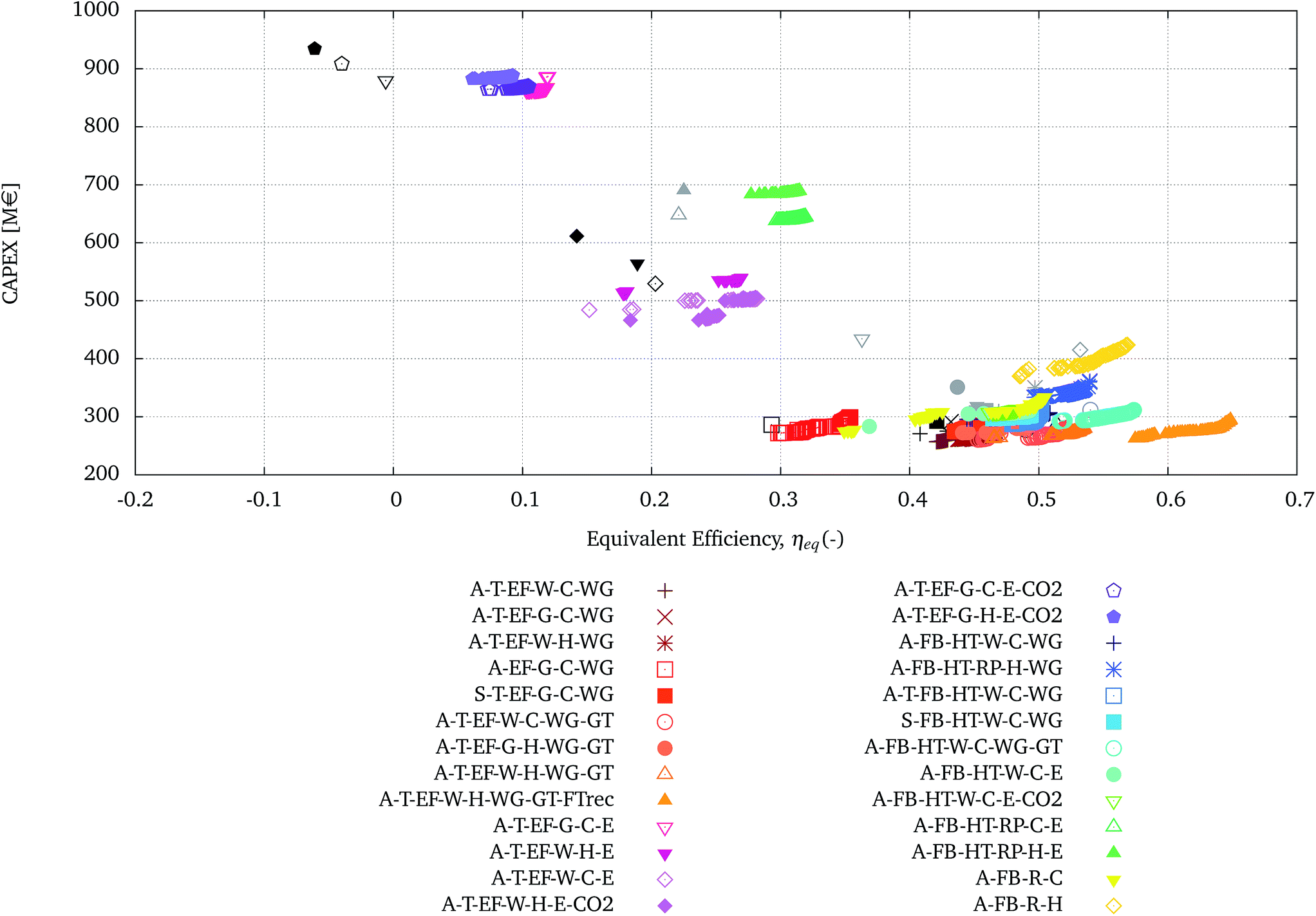Fig. 5 ‘Pareto’ solutions obtained from the multi-objective optimisation of each configuration presented in Tables 5 and 6. The initial points of each configuration, relative to the single runs, are presented in black for the configurations employing the EF gasifier and in gray for the ones employing the FICFB gasifier.

Fig. 5 also presents the results corresponding to the base-case of each configuration, in black from Table 5 and grey from Table 6. The comparison between the Pareto solutions and the base-case results clearly shows the effect of the multi-objective optimisation, in terms of improving the objective functions and extending the range of possibilities to a family of optimal solutions.

Three broad regions can be identified in Fig. 5 plotted: the top-right, centre and bottom-left.

• At the top left there are the high investment cost and low equivalent efficiency solutions, which are the ones using electrolysis with EF gasification and gas quench.

• In the centre, with intermediate values of investment cost and equivalent efficiencies, there are processes employing electrolysis with EF gasification with water quench or FICFB with radiation panels.

• At the bottom left, with the lowest investment cost and highest equivalent efficiency, there are processes employing EF, FICFB with WGS and/or tar reforming.

The processes in the bottom-right corner have similar performances and are shown with more detail in the zoomed-in graph in Fig. 6.

Fig. 6 Zoom of a section of Fig. 5 highlighting the relative performance of the optimal solutions.

It is clear that with the multi-objective optimisation, the relative positions of the single runs and Pareto solutions can change. In certain cases, the Pareto fronts cross and the relative performance can be reversed for different values of the optimisation variables. For example configuration A-FB-HT-W-C-WG () and configuration A-T-FB-HT-W-C-WG () cross at η_eq of 0.5. For values of η_eq smaller than 0.5 the second process dominates the first one, whereas for greater values of η_eq the first process is dominant. For other configurations it is possible to see that to further improve the η_eq, beyond the solutions found for a configuration, a change in the configuration itself is necessary. For example to further increase the efficiency with respect to the Pareto solutions of configuration A-T-EF-W-H-WG-GT () it is necessary to switch to configuration A-FB-HT-W-C-WG-GT ().

It should be remembered that the solutions proposed by the multi-objective optimisation maximise the η_eq, rather than the production of the FT fuel. Therefore the η_chem, even though not directly represented in the Pareto solutions, should always be taken into consideration for process comparison. Likewise, the η_en is not considered here as an objective function, but it is widely accepted and used in the industry for comparing processes and is therefore taken into account as an indicator. The η_chemversus the CAPEX and the η_enversus the CAPEX for each solution are reported in the ESI.†

3.3 Fuel produced and electricity balance

To further analyse the relative performance of the processes, Fig. 7 presents the fuel produced versus the net electricity balance (positive if exported, negative if imported) in kW of fuel or electricity per MW_th of biomass input. For different processes, the ratio between the delta of fuel produced over the delta of electricity required can be referred to as a marginal electricity to fuel efficiency.

Fig. 7 FT fuel production vs. electricity balance (positive if exported, negative if imported) of the optimised solutions presented in Fig. 5.

Most configurations displayed in Fig. 7 form a horizontal line, showing that the production of FT fuel, and consequently the η_chem, remains similar within the family of solutions. In these cases the increase in η_eq is mostly due to a better integration of the steam network which includes larger (and more expensive) steam turbines. The marginal efficiency can also vary within a family of optimal solutions. For example, the configuration A-T-EF-W-H-WG-GT-FTrec (), displaying the highest equivalent efficiencies, also displays decreasing chemical conversion efficiency with respect to the increase of electricity production, but corresponding to a very small marginal efficiency of 0.10. In this case, in certain optimal solutions, part of the synthesis gas is burnt for the production of heat and electricity, directly affecting the production of the FT fuel. For other configurations, the marginal efficiency can change abruptly within the same family of solutions, for example for A-FB-R-C when greater fractions of the synthesis gas are burnt in the processes.

Fig. 7 also highlights a general trend, across technologies, where the increasing net electricity balance corresponds to a decreasing chemical conversion efficiency. From this graph it is possible to estimate that, on average, and including all the configurations evaluated in this study, an increase of 0.84 kW_FT of FT fuel produced per MW_th of biomass corresponds to an extra electricity consumption of 1 kW_e per MW_th of biomass, and therefore a marginal efficiency of 0.84. It should be underlined that this result is significant across technologies and not within specific configurations. It is in fact a consequence of the introduction of electrolysis in the configurations and the consequent relative position of processes using HTE with respect to processes using WGS or tar reforming. The stoichiometry of the ideal reactions converting biomass to FT and the related enthalpy and Gibbs free energy balances are evaluated in ref. 55. Results show that the marginal efficiency of the ideal process (considering the Gibbs free energy balance equivalent to a net electricity balance) is about 25% lower than the marginal efficiency obtained in the present study.

3.4 Specific emissions

The specific CO₂ emissions, Em_pCO₂, versus the amount of fuel produced per MW_th of biomass are displayed in Fig. 8. The same graph reports for comparison the horizontal line representing the sum of the specific CO₂ emissions related to conventional diesel fuel generation, EmCO_2geDiesel of 36.7 kg MW h⁻¹, and combustion, EmCO_2cDiesel of 266.803 kg MW h⁻¹, as reported in Section 2.2.3.

Fig. 8 CO₂ emissions (Em_pCO₂) vs. FT fuel production of the optimised solutions presented in Fig. 5. Em_pCO₂ are presented with the same legend as presented in Fig. 5. The horizontal line represents the sum of the specific CO₂ emissions related to conventional diesel fuel generation, EmCO_2geDiesel of 36.7 kg MW h⁻¹, and combustion, EmCO_2cDiesel of 266.803 kg MW h⁻¹.

The configuration A-T-EF-W-H-WG-GT-FTrec () using recycling of the FT appears to have the lowest specific emissions. This is because the optimisation of this configuration leads to processes where the recycling ratio, R_FT, is driven to a minimum and the off-gases from the FT synthesis are used to fuel the gas turbine. The low Em_pCO₂ is due to the high electricity production (but consequent low FT fuel yield) and the corresponding displacement of electricity derived from the European electricity mix.

Again, it is possible to set the position of the processes using electrolysis aside from the rest of the configurations. In terms of Em_pCO₂, the high electricity consumption of these processes reduces the benefits from a higher conversion of biomass into FT fuel, at least considering the European context as a reference for electricity emissions. Processes using electrolysis display the highest Em_pCO₂. Electrolysis, therefore, may play an important role in BTL processes to increase biogenic carbon conversion into liquid fuels, but the emissions related to the corresponding electricity consumption should be carefully accounted for. This technology could be especially interesting in a BTL process, as a means to store renewable and low carbon electricity in the form of liquid fuels.

3.5 Cost analysis

The fuel production costs, P*, versus the capital investment, CAPEX, obtained through the multi-objective optimisation are represented in Fig. 9 against the values adapted from the literature survey of BTL techno-economic evaluations published by Haarlemmer et al.¹⁴ The literature values are scaled to a capacity of 200 MW_th using the same method illustrated by the authors. As discussed in Section 1, the comparison between different technologies and process options, on the basis of different studies, is very difficult. The underlying reasons for the dispersion of the literature values are amply analysed by^14,15 and strongly depend on the different assumptions taken into consideration. The values from the literature reported in Fig. 9 are relative to conversion pathways employing either an EF gasifier or a fluidised bed gasifier. These configurations do not include technologies designed to enhance the overall biogenic carbon conversion, such as electrolysis.

Fig. 9 The fuel production costs, P*, versus the capital investment, CAPEX of the optimised solutions presented in Fig. 5 compared to literature values. The literature values adapted from ref. 14 are displayed with +, the red dashed line represents 2σ intervals of the literature values.

Results show that the values obtained in this study, in terms of capital investments, CAPEX, and production costs, P*, are within the range of values proposed by the literature and slightly below their average. Most of the configurations appear clustered in the bottom left section of Fig. 9. Considering the uncertainties relative to the economic evaluation it is indeed difficult to differentiate, in terms of costs, between these configurations. Nevertheless, given the fact that the same modelling approach, economic evaluation method, and assumptions have been considered for each solution, it is possible to infer the general and relative trends engendered by the choice of the different technological options. Again, as expected, the solutions using HTE display the highest investment and production costs. The interest of using electrolysis depends, apart from the emissions related to the use of electricity, also on its availability at low cost and the possibility to reduce the investment relative to the Solid Oxide Electrolyser Cell (SOEC) stack.

4 Discussion

The contributions of this work are represented by the framework for the thermo-economic evaluation and optimisation of BTL conversion processes, by the database of thermochemical and economic models and by the analysis of the results with the comparison to the literature.

The modelling of the conversion of the synthesis gas to the final FT fuel takes into account several options for cleaning, cooling and composition adjustment. In particular, the possibility of reforming tars from FICFB gasification, using hot gas clean-up and adjusting the H₂/CO ratio by the external H₂ supply through HTE are represented. These processes are considered as promising and innovative technologies in the design of BTL conversion systems.

27 BTL process configurations are first analysed and then evaluated through multi-objective optimisation, maximising the η_eq and minimising the CAPEX. The results emphasise the contribution of multi-objective optimisation in the analysis of process configurations, showing that the comparison is extended to a large number of processes, belonging to the optimal solutions, that can be evaluated on the same basis. The economic analysis shows that results, in terms of production costs and CAPEX, are consistent with literature values. On the one hand, as explained earlier, because of the different assumptions considered in different literature studies, no clear trend regarding technological options can be inferred. On the other, the optimal solutions obtained in this study can be clearly distinguished in three families ranging from low to high CAPEX (and high to low η_eq): (i) processes using WGS (and not electrolysis), (ii) processes using electrolysis in combination with FICFB gasification or EF gasification with water quenching, and (iii) processes using electrolysis with EF gasification with the gas quench.

The effect of alternative technological options is analysed for each section of the conversion process and the combination of technologies, which can improve performance are highlighted. In particular, the main conclusions regarding process configurations alternatives are:

• The WGS unit operation, for gas adjustment, produces the best performing processes in terms of η_eq (0.4 < η_eq < 0.65) and CAPEX (<350 M€ for 200 MW_th plant capacity), with intermediate to low conversion efficiencies (0.1 < η_chem < 0.5).

• FICFB gasification, in configurations using the WGS unit operation, yields slightly higher η_eq efficiencies with respect to EF gasification. However the CAPEX of processes using EF gasification are generally slightly lower.

• HTE introduces the greatest impact on process performance.

• The configurations employing HTE are always sub-optimal with respect to more conventional processes, in terms of the objectives considered in this study, with low η_eq (0.05 < η_eq < 0.4) and high CAPEX (450 M€ < CAPEX < 900 M€, for 200 MW_th plant capacity). Nevertheless, HTE provides significant improvements in terms of the conversion of biomass into fuel, η_chem (0.5 < η_chem < 0.8).

• The introduction of HTE allows, on average, 84% additional energy in the FT fuel output produced with respect to the additional input energy in the form of electricity (the marginal efficiency).

• The highest conversion of biomass into FT fuels, up to slightly over 0.8 kJ_FT kJ_th⁻¹, is obtained by configurations which combine HTE with EF gasification and gas quenching. These configurations avoid the WGS reaction along the process the most, reducing therefore the amount of carbon lost in the form of CO₂.

• Electricity requirement to grind raw biomass is the bottle neck for the improvement of the yield of processes using EF gasification. This electricity requirement should be reduced significantly, about fivefold, to avoid torrefaction and obtain similar values of η_eq.

• The use of tar reforming, avoiding the WGS and HTE unit operations, improves the η_eq of the base-case configuration, employing FICFB gasification, a high temperature stage, water quench, WGS, and cold gas clean-up, when used in combination with the hot gas clean-up. The η_eq increases from a maximum of slightly over 0.50 to about 0.57 with a corresponding increase in CAPEX from about 300 to 420 M€.

In this context, several improvements could be especially interesting, both in terms of model detail and concepts that could require further analysis in a future evaluation. Some of the improvements could be:

• The superstructure could be extended considering other unit operations as shown in Fig. 2 and to include several syngas to fuels and chemicals options, as evaluated for example by ref. 56.

• The process integration could be carried out considering the design and synthesis of the Heat Exchanger Network (HEN).⁵⁷

• A thorough analysis of the effect of the uncertainty of model parameters, investment cost estimates and the price of resources should be included in this study. Work on the application of global sensitivity analysis in multi-objective optimisation is carried out, for example, by ref. 58. The best configurations and processes under uncertain market conditions could be determined using the methodology developed by ref. 59 in the context of CO₂ capture.

• It would be interesting to analyse the effect of the definition of the objectives on the solutions proposed, and in particular the electricity to fuel equivalent defined in this study. Given the trade-off observed in the analysis of the results in terms of electricity balance and FT produced, the maximisation of the ratio of the fuel produced over the net electricity consumed is proposed as an objective.

5 Conclusions

In this study, it has been clearly shown that there are many possible ways to configure and evaluate BTL process chains. Results show three different families of solutions: (i) EF, FICFB with WGS and/or tar reforming, (ii) EF with water quench, FICFB with radiation panels and electrolysis, (iii) EF with gas quench and electrolysis. Their performances, in terms of the indicators analysed in this study, are summarised in Table 7.

Table 7 Summary of performances

	η eq	η chem	Elec. balance [kWe MWth^−1]	CAPEX [M€]	P* [€^−1]	EmpCO2 [kgCO2 MW hFT^−1]
(i) EF, FICFB with WGS and/or tar reforming	[0.4, 0.65]	[0.1, 0.48]	[−100, +350]	[250, 350]	[1, 1.4]	[80, −1000]
(ii) EF with water quench, FICFB with radiation panels and electrolysis	[0.15, 0.3]	[0.52, 0.7]	[−150, −250]	[450, 700]	[1.5, 1.6]	∼100
(iii) EF with gas quench and electrolysis	[0.05, 0.1]	∼0.8	[−400, −450]	880	1.8	∼200

---

The cheapest processes with the highest efficiencies belong to the families of solutions (i) and (ii), whereas processes that maximise the chemical conversion of biomass into the final fuel (η_chem) belong to the family of solutions (iii) which use electrolysis to add H₂ to the process. In terms of CO₂ emissions, considering the average European electricity mix, processes belonging to family (iii) display emissions per unit of fuel produced approaching that of conventional diesel (266.803 kg MW h⁻¹). These processes can therefore become interesting to reduce CO₂ emissions when they use low carbon intensity electricity (e.g. the French electricity mix) or carbon neutral electricity.

To conclude, this study formulated a coherent and complete framework for multi-objective evaluations, which can be a decision-support tool in the design of a BTL conversion facility. The results should be analysed critically, considering several indicators of interest. They do not provide a single best configuration, but highlight the trade-offs between different technological options.

Conflicts of interest

There are no conflicts to declare.

Acknowledgements

The research for this paper was in part financially supported by the Commissariat à l'énergie atomique et aux énergies alternatives of Grenoble (CEA-Grenoble) in France and in part by the Swiss Competence Center for Energy Research BIOSWEET – Biomass for Swiss Energy Future. The authors would also like to thank Shivom Sharma for providing useful input for the revision of the manuscript.

References

1. International Energy Agency, World Energy Outlook 2012, IEA Technical Report, 2012.
2. G. Berndes, M. Hoogwijk and R. van den Broek, Biomass Bioenergy, 2003, 25, 1–28.
3. International Energy Agency, Transport, Energy and CO₂, 2009.
4. International Energy Agency, CO₂ Emissions From Fuel Combustion – Highlights, 2011.
5. International Energy Agency, Energy Technology Perspectives 2010, scenarios and strategies to 2050, IEA publications, Paris, France, 2010.
6. Development Policy Review Network, http://www.agrofuelsplatform.nl, 2012.
7. C. A. Floudas, J. A. Elia and R. C. Baliban, Comput. Chem. Eng., 2012, 41, 24–51.
8. A. S. Snehesh and S. Dasappa, Renewable Sustainable Energy Rev., 2016, 58, 267–286.
9. A. S. Snehesh, H. S. Mukunda, S. Mahapatra and S. Dasappa, Energy, 2017, 130, 182–191.
10. M. Patel, X. Zhang and A. Kumar, Renewable Sustainable Energy Rev., 2016, 53, 1486–1499.
11. V. S. Sikarwar, M. Zhao, P. Clough, J. Yao, X. Zhong, M. Z. Memon, N. Shah, E. J. Anthony and P. S. Fennell, Energy Environ. Sci., 2016, 9, 2939–2977.
12. X. Zhang, Green Chem., 2016, 18, 5086–5117.
13. Y.-D. Kim, C.-W. Yang, B.-J. Kim, J. Moon, J.-Y. Jeong, S.-H. Jeong, S.-H. Lee, J.-H. Kim, M.-W. Seo, S.-B. Lee, J.-K. Kim and U.-D. Lee, Appl. Energy, 2016, 180, 301–312.
14. G. Haarlemmer, G. Boissonnet, J. Imbach, P.-A. Setier and E. Peduzzi, Energy Environ. Sci., 2012, 5, 8445.
15. G. Haarlemmer, G. Boissonnet, E. Peduzzi and P.-A. Setier, Energy Environ. Sci., 2012, 5, 8445–8456.
16. J. A. Elia, R. C. Baliban and C. A. Floudas, Ind. Eng. Chem. Res., 2010, 7371–7388.
17. R. C. Baliban, J. A. Elia and C. A. Floudas, Comput. Chem. Eng., 2011, 35(9), 1647–1690.
18. R. C. Baliban, J. A. Elia, R. Misener and C. A. Floudas, Comput. Chem. Eng., 2012, 42, 64–86.
19. A. M. Niziolek, O. Onel, J. A. Elia, R. C. Baliban, X. Xiao and C. A. Floudas, Ind. Eng. Chem. Res., 2014, 140507101404002.
20. M. Martín and I. E. Grossmann, Comput. Chem. Eng., 2011, 35, 1798–1806.
21. M. Martín and I. E. Grossmann, Ind. Eng. Chem. Res., 2011, 50, 13485–13499.
22. M. Martín and I. E. Grossmann, AIChE J., 2011, 57, 3408–3428.
23. M. Gassner and F. Maréchal, Comput. Chem. Eng., 2009, 33, 769–781.
24. M. Gassner, Process design methodology for thermochemical production of fuels from biomass, Application to the production of synthetic natural gas from lignocellulosic resources, École Polytechnique Fédérale de Lausanne, Switzerland, 2010.
25. L. Gerber, M. Gassner and F. Maréchal, Comput. Chem. Eng., 2011, 35, 1265–1280.
26. M. Gassner and F. Maréchal, Energy Environ. Sci., 2012, 5, 5768–5789.
27. L. Tock and F. Maréchal, Comput. Chem. Eng., 2014, 61, 51–58.
28. T. Yee and I. Grossmann, Comput. Chem. Eng., 1990, 14, 1165–1184.
29. F. Maréchal and B. Kalitventzeff, Comput. Chem. Eng., 1998, 22, S149–S156.
30. L. Tock, M. Gassner and F. Maréchal, Biomass Bioenergy, 2010, 34, 1838–1854.
31. R. Bolliger, PhD thesis, École Polytechnique Fédérale de Lausanne, Lausanne, 2010.
32. F. Maréchal and B. Kalitventzeff, Comput. Chem. Eng., 1996, 20, 225–230.
33. F. Maréchal and B. Kalitventzeff, Comput. Chem. Eng., 1999, 23, s133–s136.
34. S. A. Belsim, Belsim Vali, 2013, http://www.belsim.com.
35. A. Molyneaux, PhD thesis, École Polytechnique Fédérale de Lausanne, 2002.
36. A. Molyneaux, G. Leyland and D. Favrat, Energy, 2010, 35, 751–758.
37. U.S. Energy Information Agency, Average annual heat rates for specific types of fossil-fuel generators and nuclear power plants, 2014, http://www.eia.gov.
38. GE Energy, Heavy duty gas turbine products, 2014, http://www.ge-energy.com/.
39. Siemens, Efficiency Record of Combined Cycle Power Plant, 2014, http://www.siemens.com.
40. J. Szargut, D. R. Morris and F. R. Steward, Exergy analysis of thermal, chemical, and metallurgical processes, Hemisphere, 1988, p. 332.
41. Q. Bernical, X. Joulia, I. Noirot-Le Borgne, P. Floquet, P. Baurens and G. Boissonnet, Ind. Eng. Chem. Res., 2013, 52, 7189–7195.
42. P. L. Cruz, D. Iribarren and J. Dufour, Fuel, 2017, 194, 375–394.
43. A. Chauvel, G. Fournier and C. Raimbault, Manuel d'évaluation économique des procédés, 2001, p. 488.
44. R. Turton, B. Richard C, B. W. Wallace and S. A. Joseph, Analysis, Synthesis, and Design of Chemical Processes, Prentice Hall, 2nd edn, 2002, p. 987.
45. G. D. Ulrich and T. V. Palligarnai, Chemical Engineering Process Design and Economics, a Practical Guide [Hardcover], Process Publishing, 2nd edn, 2004, p. 706.
46. J. P. Ros, J. G. van Minnen and E. J. Arets, Climate effects of wood used for bioenergy, Pbl/alterra note technical report, 2013.
47. Swiss Centre for Life Cycle Inventories, Ecoinvent, 2007, http://www.ecoinvent.ch.
48. B. Steubing, I. Ballmer, M. Gassner, L. Gerber, L. Pampuri, S. Bischof, O. Thees and R. Zah, Renewable Energy, 2014, 61, 57–68.
49. O. P. R. Van Vliet, A. P. C. Faaij and W. C. Turkenburg, Energy Convers. Manage., 2009, 50, 855–876.
50. C. Hamelinck, A. Faaij, H. Denuil and H. Boerrigter, Energy, 2004, 29, 1743–1771.
51. M. Gassner and F. Maréchal, Biomass Bioenergy, 2009, 33, 1587–1604.
52. E. Peduzzi, G. Boissonnet, G. Haarlemmer, C. Dupont and F. Maréchal, Energy, 2014, 70, 58–67.
53. E. Peduzzi, G. Boissonnet and F. Maréchal, Fuel, 2016, 181, 207–217.
54. J. Van herle, F. Maréchal, S. Leuenberger and D. Favrat, J. Power Sources, 2003, 118, 375–383.
55. E. Peduzzi, G. Boissonnet and F. Maréchal, Comput.-Aided Chem. Eng., 2016, 38, 1893–1898.
56. N. L. Truong and L. Gustavsson, Appl. Energy, 2013, 104, 623–632.
57. A. Mian, E. Martelli and F. Maréchal, Ind. Eng. Chem. Res., 2016, 55, 168–186.
58. S. Fazlollahi, Decomposition optimization strategy for the design and operation of district energy systems, École Polytechnique Fédérale de Lausanne, Switzerland, 2014.
59. L. Tock and F. Maréchal, 24th European Symposium on Computer Aided Process Engineering -ESCAPE24, Budapest, Hungary, 2014.

---

Footnotes

† Electronic supplementary information (ESI) available. See DOI: 10.1039/c7se00468k

‡ Critical reviews are provided for example by Floudas et al.,⁷ Snehesh et al.,^8,9 Patel et al.,¹⁰ Sikarwar et al.¹¹ and Zhang et al.,¹² whereas the research status in terms of biomass BTL processes is reported by Kim et al.¹³

§ Liquid bio-hydrocarbons that are functionally equivalent to petroleum fuels and, as such, compatible with the existing petroleum infrastructure.

¶ The process under investigation is, in this case, biomass to synthetic natural gas.

---