
 Open Access Article
 This Open Access Article is licensed under a Creative Commons Attribution-Non Commercial 3.0 Unported Licence
Structural–elastic determination of the force-dependent transition rate of biomolecules†
Shiwen
Guo‡
a,
Qingnan
Tang‡
b,
Mingxi
Yao
a,
Huijuan
You
c,
Shimin
Le
b,
Hu
Chen
d and
Jie
Yan
 *abe
*abe
aMechanobiology Institute, National University of Singapore, Singapore 117411. E-mail: phyyj@nus.edu.sg; Fax: +65-6777-6126; Tel: +65-6516-2620
bDepartment of Physics, National University of Singapore, Singapore 117551
cSchool of Pharmacy, Tongji Medical College, Huazhong University of Science and Technology, Wuhan, China 430030
dDepartment of Physics, Xiamen University, Xiamen, China 361005
eCentre for Bioimaging Sciences, National University of Singapore, Singapore 117557
First published on 29th May 2018
Abstract
The force-dependent unfolding/refolding of protein domains and ligand-receptor association/dissociation are crucial for mechanosensitive functions, while many aspects of how force affects the transition rate still remain poorly understood. Here, we report a new analytical expression of the force-dependent rate of molecules for transitions overcoming a single barrier. Unlike previous models derived in the framework of Kramers theory that requires a presumed one-dimensional free energy landscape, our model is derived based on the structural–elastic properties of molecules which are not restricted by the shape and dimensionality of the underlying free energy landscape. Importantly, the parameters of this model provide direct information on the structural–elastic features of the molecules between their transition and initial states. We demonstrate the applications of this model by applying it to explain force-dependent transition kinetics for several molecules and predict the structural–elastic properties of the transition states of these molecules.
1 Introduction
It has been known that single cells can sense the mechanical properties of their micro-environment and transduce the mechanical cues into biochemical reactions that eventually affect the cell shape, migration, survival, and differentiation.1 This mechanotransduction requires transmission of force through a number of mechanical linkages, each of which is often composed of multiple linearly arranged force-bearing proteins that are non-covalently linked to one another. Under force, the domains in each protein in the linkage may undergo transitions between folded and unfolded states. In addition, two neighbouring proteins in the linkage can dissociate and re-associate under force. Therefore, the force-dependent transition rates of protein domains and protein–protein complexes is a key factor that affects mechanotransduction on a particular mechanical linkage. Determining the force-dependent transition rate of biomolecules has been the focus of experimental measurements2–7 and theoretical modelling.8–18 Previous single-molecule force spectroscopy measurements have revealed complex kinetics for a variety of molecules,2–6 yet the mechanisms still remain elusive.An extensively applied phenomenological expression of k(F) was proposed by Bell et al.:8k(F) = k0eβFδ*, where β = (kBT)−1, k0 is the rate in the absence of force and δ* is the constant transition distance. This model assumes that the force applied to the molecule results in change of the energy barrier by the amount of −Fδ*, while the physical basis of this assumption is weak. The limitation of Bell's model has been revealed in many recent experiments that reported complex deviations from its predictions.2–6
In order to explain such deviations, several analytical expressions of k(F) were derived based on extending Brownian dynamics theory from Kramers19 for force-dependent dissociation of bonds.9–12 Kramers theory was originally proposed to study the kinetics of particles escaping from an energy well through diffusion on a presumed one-dimensional free energy landscape. This theory shows that for a sufficiently high barrier, the escaping rate exponentially decreases with the height of the barrier, which proves the Arrhenius law for the one dimensional case. k(F) in the framework of Kramers theory is derived based on a force-dependent free energy landscape U(x) = U0(x) − Fx, where U0(x) is a fixed zero force free energy landscape and x is the extension change of the molecule during the transition. Assuming a sufficiently high energy barrier such that the energy well and the barrier are well separated and for the cases where U0(x) can be approximated by a cusp or a linear–cubic function, an analytical expression of k(F) was derived,11 which has been extensively applied to explain experimental data.
In general, the applications of the expression of k(F) derived based on the framework of Kramers theory are limited by three factors, namely (1) the assumption that the transition pathway is one dimensional, (2) the assumption that the molecular extension change is a good transition coordinate, and (3) the shape of the presumed free energy surface U0(x). A more recent publication20 shows that k(F) can be re-expressed as  in the framework of Kramers theory, where δ*(F) is the average extension difference of the molecule between its transition state and native state. This expression does not have an explicit dependence on a presumed free-energy landscape U0(x). However, in order to actually apply this formula, a presumed one-dimensional free energy landscape is still needed to calculate δ*(F). Due to these limitations, although k(F) derived in the framework of Kramers theory can explain mild deviations from Bell's model,10–12 they typically predict monotonic k(F) and fail to explain more complex experimentally observed kinetics, such as the non-monotonic k(F) reported in several recent experiments.2,3,5
Previously, non-monotonic k(F) was typically explained by high-dimensional phenomenological models involving multiple competitive pathways or force-dependent selection of multiple native conformations that have access to different pathways.13–17 For example, the transition rate described by two competitive transition pathways, k(F) = k1(F) + k2(F), each following Bell's model, can explain non-monotonic k(F) with one of the transition distances being negative.13 On the other hand, models based on force-dependent selection of multiple native conformations that have access to different pathways are much more complex and lack analytical simplicity for general cases.14 Simplification of such models must require additional assumptions on the force-dependence of the selection of native conformations.14–16 A limitation of all these models is that model parameters do not provide insights into the structural and physical properties of the molecules in their native and transition states.
We recently reported that k(F) of mechanical unfolding of titin I27 immunoglobulin (Ig) domain exhibits an unexpected “catch-to-slip” behaviour at low force range.2 It switches from a decreasing function (i.e., “catch-bond” behaviour) at forces below 22 pN to an increasing function (i.e., “slip-bond” behaviour) at forces greater than 22 pN. The transition state of the titin I27 domain is known to involve a peeled A–A′ peptide containing 13 residues.21–24 Taking advantage of the known structures of I27 in its native and transition states, we analysed the effects of the structural–elastic properties of I27 on its force-dependent unfolding kinetics by applying the Arrhenius law. We demonstrated that the entropic elasticity of titin I27 in the two states is responsible for the observed “catch-to-slip” behaviour of k(F). Besides suggesting the structural–elastic properties of a molecule as a critical factor affecting the force-dependent transition rate, the results also point to a possibility of deriving k(F) based on the structural–elastic properties of molecules in the framework of the Arrhenius law. As the derivation of k(F) based on the Arrhenius law does not depend on any presumed free energy landscape, it is not limited by the dimensionality of the system and the choice of the transition coordinate.
The results described in our previous work2 are obtained based on the prior knowledge of the structural–elastic properties of I27 in its native and transition states. Unfortunately, such prior knowledge is unavailable for most of the other molecules. In order to interpret the force-dependent transition rate based on the structural–elastic properties of molecules for generic cases, it is necessary to derive an expression of k(F) that contains parameters related to the potential structural–elastic properties of the molecule based on the Arrhenius law. If this can be achieved, fitting the experimental data using the derived k(F) not only can be applied to explain experimental data but also can provide important insights into the structural–elastic properties of the molecule based on the best-fitting values of the model parameters. To our knowledge, k(F) with such capability has not been derived before.
2 Results
2.1 Deriving k(F) based on the structural–elastic properties of molecules
 | ||
| Fig. 1 The force-dependent conformation free energies of the native, the transition and the denatured states: The native state is sketched as a folded structure, with a length of b0 and stretching rigidity of γ0. The transition state is modelled as a structure consisting of a folded core with a length of b* and stretching rigidity of γ* as well as a flexible polymer with a contour length of L*. The denatured state is a flexible polymer with a contour length of L0. The force directions are indicated by black arrows, and the force-attaching points on the native state and on the folded core in the transition state are indicated by red dots. The formula of the force-dependent conformation free energies of these states is provided. | ||
The native state and the folded core in the transition state are modelled as a deformable folded structure. The relaxed length of the structure is defined as the linear distance between the two force-attaching points on the folded structure in the absence of force (Fig. 1). Here a deformable folded structure refers to slight deformation along the force direction without causing local structural changes. One example is the B-form DNA, which can be extended beyond its relaxed contour length without breaking any Watson–Crick base pairs in the force range of 20–40 pN.25,26
We assume that a folded structure with a relaxed length b can only undergo small tensile deformation around the energy minimum approximated by a harmonic potential with a spring constant κ. The tensile deformation Δb relative to the relaxed length b is proportional to the applied force F and inversely proportional to the stretching rigidity γ, i.e., Δb/b = F/γ. It can be seen that κ = γ/b. Hereafter we define the stretching deformability of a rigid structure as b/γ, which is the reciprocal of κ. The stretching rigidity γ is in the order of 102–103 pN for typical protein domains and nucleic acid structures (ESI: SI and SII, Table S1†). We note that since protein domains are highly anisotropic, the value of γ should be dependent on the direction of stretching. The same protein domain may have very different values of γ between two different choices of sites to apply force.
Force F introduces an entropic conformation free energy Φ(F) to a molecule in a particular structural state, in addition to other chemical interactions that maintain the molecule in the structural state. Φ(F) can be calculated based on the force–extension curve of the molecule x(f) as:  (ref. 27 and 28) (ESI: SIII†). A deformable folded structure with a relaxed length of b and a stretching rigidity γ has a very simple analytical force–extension curve,29
 , where
  is the solution of the force–extension curve of an inextensible rod with a length of b. The factor
  takes into account the force-dependent tensile deformation of the rod. The force–extension curve of a peptide or ssDNA/ssRNA polymer can be described by the worm-like chain (WLC) polymer model that contains two parameters, the bending persistence length A and the contour length L = nlr. Here n is the number of residues in the polymer and lr is the contour length per residue. The value of A is fixed for a given molecule under given solution conditions. Based on the WLC model, xL(f) can be obtained by solving the inverse function of the Marko–Siggia formula:30
 .
.
By integration of the force–extension curves, the force-dependent entropic conformation free energy scaled by β−1 = kBT for a deformable folded structure and a polymer have the following analytical solutions:
 | (1) |
 is the second order polylogarithm function (also known as Jonquire's function) and ξ(2) ∼ 1.645 is the Riemann-zeta function evaluated at z = 2.
 | (2) |
 , which can be rewritten as a linear combination of three terms:
 | (3) |
The force-dependent unfolding/dissociation rate is then determined by applying the Arrhenius law,  :
:
 | (4) |
At forces ≫kBT/b0, ≫kBT/b* and ≫kBT/A, ku(F) has a simple asymptotic expression:
 | (5) |
![[k with combining tilde]](https://www.rsc.org/images/entities/i_char_006b_0303.gif) u,0 and three model parameters
u,0 and three model parameters  ,
,  , and
, and  . Typical values of
  and
and  are in the range of 10−3 nm to 10−2 nm (ESI: SI and SII, Table S1†); therefore, σ ∼ L* + (b* − b0). An alternative derivation of eqn (5) is provided in the ESI (SIV: “Alternative derivation of eqn (5)”).† Here we emphasize that, since eqn (5) is a large-force asymptotic formula, u,0 should not be interpreted as the zero-force transition rate. The zero-force rate ku,0 predicted by the model should be based on eqn (4), which is related to u,0 using the following equation:
 | (6) |
Clearly, in the three model parameters of eqn (5), σ is the contour length difference, and α describes the deformability difference between the folded core of the transition state and the native state. η only depends on the contour length of the flexible polymer in the transition state. Eqn (5) therefore relates the force dependence of unfolding/dissociation rates to the differential structural–elastic properties of molecules between their native and transition states. The native state structure is often known, and therefore b0 is determined. In addition, with the known native state structure, γ0 can be estimated with reasonable accuracy using all-atom molecular dynamics (MD) simulations (ESI: SI and SII†). Hence, for molecules with a known native state structure, the structural–elastic parameters of the transition state can be solved from σ, α and η. As a result, it is possible to obtain further insights into the structural–elastic properties of the transition state based on the best-fitting values of σ, α and η.
 , where the subscript r indicates refolding transition. Since refolding typically occurs at low force range (a few pN for protein domains6,32,33), the force-dependent deformation of the folded core in the transition state can be ignored. Therefore, γ* can be set as infinity, and as a result
  . In addition, since the force extension curve of a polymer is proportional to the polymer contour length, the term xL*(F) − xL0(F) can be rewritten as: −xL0−L*(F). Finally, we can rewrite the force-dependent refolding transition distance as:
 | (7) |
The resulting force-dependent free energy barrier change, 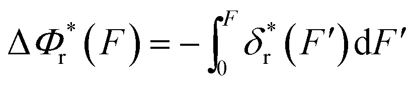 , has a simple analytical solution as:
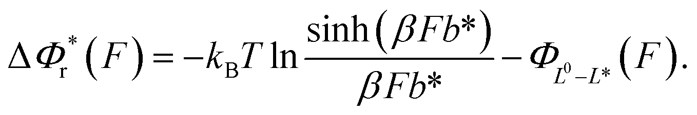 | (8) |
By applying the Arrhenius law, the force-dependent refolding rate can be expressed as:
 | (9) |
L 0 is typically known based on the number of residues for given protein domains or nucleic acid structures. Therefore, fitting experimental data using eqn (9) can determine b* and L* which are associated with the transition state structure.
 | (10) |
In this equation, r > 0 and r < 0 indicate force-increase and force-decrease processes, respectively, during which unfolding and refolding occur at certain forces. The initial force F0 should be chosen to ensure ∼1 probability of the folded state and unfolded state at the force, for the unfolding experiment with r > 0 and the refolding experiment with r < 0, respectively. p(F) in eqn (10) is a probability density function, and therefore the transition force histogram obtained from experiments should be reconstructed as 〈number of counts per bin〉/〈the total number of counts〉/〈bin size〉.
2.2 Applications in interpreting experimental data
 | ||
Fig. 2 Unzipping and rezipping force distributions of DNA hairpin: (A) A 15 bp DNA hairpin containing a 15 nt poly-T terminal loop spanning between two dsDNA handles is subject to forces applied using magnetic tweezers. (B) The unzipping and rezipping transitions during force increase (r = 2.0 ± 0.2 pN s−1) and force decrease (r = −2.0 ± 0.2 pN s−1) are indicated by abrupt extension changes which are denoted by arrows. (C) Unzipping force distribution (dark grey bars) constructed from 202 unfolding events and rezipping force distribution (light grey bars) constructed from 192 refolding events from 9 independent DNA tethers. The data are fitted using eqn (10) based on eqn (5) for unzipping and eqn (9) for rezipping (black dashed curves). The data are also fitted using eqn (10) based on Bell's model (grey dotted curves) for comparison. (D)  calculated with eqn (2) (solid line) and calculated with eqn (2) (solid line) and  calculated with eqn (3) (dash-dot line) for DNA hairpin unzipping. (E) calculated with eqn (3) (dash-dot line) for DNA hairpin unzipping. (E)  calculated with eqn (7) (solid line) and calculated with eqn (7) (solid line) and  calculated with eqn (8) (dash dot line) for DNA hairpin rezipping. (F) The predicted ku(F) (solid line) and kr(F) (dashed line) based on the parameters determined by fitting to the unzipping and rezipping force distributions. calculated with eqn (8) (dash dot line) for DNA hairpin rezipping. (F) The predicted ku(F) (solid line) and kr(F) (dashed line) based on the parameters determined by fitting to the unzipping and rezipping force distributions. | ||
In the case of DNA unzipping, the transition state should correspond to a structure with a certain number (n*) of single-stranded DNA nucleotides under force. In 100 mM KCl, the ssDNA has a persistence length of A ∼ 0.7 nm and a contour length per nucleotide of lr ∼ 0.7 nm according to previous studies34 and confirmed in our study (ESI: SV†). The native state and the rigid body fraction in the transition state are the same, γ0 = γ* and b0 = b* ∼ 2 nm (i.e., the diameter of B-form DNA, see sketch in Fig. S10†). Therefore, the parameter α = 0 nm pN−1. As a result, the shape of ku(F) only depends on σ = L* and 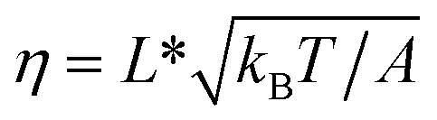 . It is easy to see that eqn (5) is reduced to a very simple form
  . Substituting this expression into eqn (10), we fitted the DNA unzipping force distribution.
As shown in Fig. 2C, the experimentally constructed p(F) can be well fitted with eqn (10) (dashed line) based on ku(F) predicted by our model with the following best-fitting parameters ku,0 = 0.005 ± 0.001 s−1, with a 95% confidence bound of (0.0003, 0.009) s−1; and L* = 10.0 ± 0.4 nm, with a 95% confidence bound of (8.4, 11.6) nm. Here, the errors indicate standard deviations obtained with bootstrap analysis (ESI: SVI†), and the 95% confidence bounds are determined by fitting of all the data points (Fig. 2C, dark grey bars). Considering lr ∼ 0.7 nm for ssDNA, the result implies ∼14 nt of ssDNA under force in the transition state, or alternatively ∼7 unzipped DNA basepairs. In order to compare with Bell's model, we also fitted the same data set using Bell's model (dotted line), with the following fitting parameters kBellu,0 ∼ 6 × 10⁻⁷ s−1 and  . As shown by this example, both models can fit the data very well.
In order to compare the transition state structures predicted by the models, we need to convert the best fitting value of  based on Bell's model into the contour length of ssDNA in the transition state. Since the transition distance is in general a function of force, a rough estimation of the contour length in the transition state can be done by converting
  into the contour length at the peak force Fp of ∼ 10 pN by solving the following equation,
  . Through this conversion, a contour length of ∼10.5 nm is estimated based on the fitting by Bell's model, which is very close to the value of L* estimated based on our model. This example shows that for simple cases such as DNA unzipping, our model and Bell's model do not exhibit significant difference. This is not surprising since Bell's model is a special case of eqn (5) when the first term in the exponential of eqn (5) is predominant.
We also fitted the rezipping force distribution of the same DNA hairpin obtained at a loading rate of r = −2.0 ± 0.2 pN s−1 (light grey bars, Fig. 2C) using eqn (10) based on Bell's model (Fig. 2C, grey dotted line) and our model (eqn (9)) (Fig. 2C, black dashed line) with L0 = 45 × lr ∼ 32 nm and b* ∼ 2 nm. Both models can fit the data well with the following fitting parameters (kBell0 = 4331 s−1;  ) for Bell's model and (kr,0 = 147 ± 39 s−1, with a 95% confidence bound of (63, 198) s−1; L* = 14.9 ± 0.8 nm, with a 95% confidence bound of (12.2, 15.5) nm) for our model. Here, the errors indicate standard deviations obtained with bootstrap analysis (ESI: SVI†), and the 95% confidence bounds are determined by fitting of all the data points (Fig. 2C, light grey bars). The best-fitting value of L* ∼ 14.9 nm from our model suggests that there are ∼21 nt of ssDNA under tension in the transition state, corresponding to ∼11 bp of unzipped DNA basepairs. Based on the best-fitting value of
  from Bell's model, about 22 nt of ssDNA are absorbed into the transition state structure according to the ssDNA force–extension curve estimated at the peak force (∼5 pN), leaving 23 nt of ssDNA under tension corresponding to ∼12 bp of unzipped DNA basepairs, which is similar to the prediction by our model. These results suggest that eqn (9) derived based on the structural–elastic properties of molecules can be used to explain the force-dependent rate of refolding. In the case of DNA rezipping, both eqn (9) and Bell's model can reasonably explain the experimental data and provide useful information on the transition state structure.
Based on L* ∼ 10 nm determined for DNA unzipping and (L0 ∼ 32 nm, b* ∼ 2 nm, L* ∼ 15 nm) for DNA rezipping, the force-dependent transition distances  and the change of the free energy barrier
  can be computed using eqn (2) and (3) for unzipping (Fig. 2D) and eqn (7) and (8) for rezipping (Fig. 2E). Here, the subscript i indicates unzipping with i = u or rezipping with i = r transitions. The results show that, for the DNA unzipping transition,
  is a positive and monotonically increasing function which results in a monotonically decreasing
  . In contrast, for the DNA rezipping transition,
  is a monotonically decreasing function which leads to monotonically increasing
  . The force-dependent transition rates calculated using
  for the respective transitions (Fig. 2F) show that force monotonically speeds up unzipping while it monotonically slows down rezipping. In addition, for both unzipping and rezipping transitions, the nonlinear profiles of ki(F) on the logarithmic scale reveal minor deviation from Bell's model. ku(F) and kr(F) curves cross at Fc ∼ 8.9 pN, predicting that at this force the unzipped and zipped states have equal probabilities, which is close to the value determined by constant force equilibrium measurements reported in our previous paper on the same DNA within ∼1 pN (Fig. S4 in ref. 35).
The titin I27 domain has a known transition state structure, which allows us to examine the quality of the prediction of the transition state properties based on the best-fitting parameters. As described earlier, the experimental data of I27 exhibits a “catch-to-slip” switching behaviour, where ku(F) switches from a decreasing function to an increasing function when the force exceeds a certain threshold value at around 22 pN (Fig. 3A, black squares).2 At forces larger than ∼60 pN, the force-dependent unfolding rate converges to a Bell-like behaviour (Fig. 3A). The best-fitting parameters according to eqn (5) without any restriction are determined as: u,0 = 0.03 ± 0.01 s−1, with 95% confidence bounds of (−0.02, 0.07) s−1; σ = 1.1 ± 0.2 nm, with 95% confidence bounds of (0.5, 1.7) nm; α = 0.002 ± 0.003 nm pN−1, with 95% confidence bounds of (−0.004, 0.007) nm pN−1; and η = 10.5 ± 1.5 nm pN1/2, with 95% confidence bounds of (6.4, 14.7) nm pN1/2. Here, the errors indicate standard deviations obtained with bootstrap analysis (ESI: SVI, Table S2†), and the 95% confidence bounds are determined by fitting of all the data points (Fig. 3A, black squares). We also tested the robustness of the convergence of the fitting by repeating the fitting procedure with 10 different well-separated initial sets of values and found that the best-fitting parameters converged to the same set regardless of the initial values (ESI: SVII, Table S5†).
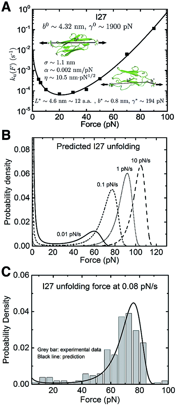 | ||
| Fig. 3 Application of eqn (5) to interpret the experimental data of titin I27: (A) The ku(F) data for titin I27 domain unfolding2 are indicated with black squares and fitted with eqn (5) (black line). The goodness-of-fit was evaluated using a R-square of ∼0.997 and a root mean squared error (RMSE) of ∼0.162. The best-fitting model parameters and the structural–elastic parameters determined based on the native state structure and steered MD simulations, or solved from the best-fitting parameters are indicated in the panel. (B) The panel shows the predicted I27 unfolding force distribution p(F) using eqn (10) based on the best-fitting parameters for ku(F), at different loading rates of 0.01 pN s−1 (solid line), 0.1 pN s−1 (short dash line), 1 pN s−1 (short dot line) and 10 pN s−1 (dash line). (C) Comparison between the predicted p(F) of I27 (solid black curve) and the experimental data (grey bars) shows good agreement at a loading rate of 0.08 pN s−1. | ||
Based on the structure of I27 and steered MD simulations, b0 ∼ 4.32 nm and γ0 ∼ 1900 pN were estimated (ESI: SI and SII, Fig. S2 and S6†). From the best-fitting parameters, L* = 4.6 ± 0.7 nm, b* = 0.8 ± 0.4 nm and γ* = 194 ± 41 pN were solved for the transition state. The value of L* corresponds to a peptide of 12 ± 2 residues, which is in good agreement with the previously known result that the transition state of I27 involves a peeled A–A′ peptide chain of 13 residues (ESI: Fig. S2†).2,21–24 This result shows that our model indeed can provide information on the structural–elastic properties of the transition state. The zero-force transition rate predicted by the model is estimated to be ku,0 ∼ 5 × 10⁻³ s−1 according to eqn (6). This value is consistent with that recently reported in ref. 2 but differs from the value extrapolated based on Bell's model in earlier studies37 (see discussions in the Discussion section).
Based on the best-fitting parameters, one can predict the I27 unfolding force probability density function p(F) using eqn (10) at any loading rate. Fig. 3B shows predicted p(F) at several loading rates from 0.01 pN s−1 to 10 pN s−1. We next compare the predicted p(F) of I27 with experiments. Previous AFM experiments suggest that the native state of I27 transits to an intermediate state with the A strand being detached from the B strand at forces >100 pN, and unfolding transition starts from this intermediate state at forces above 100 pN.38 Since the ku(F) data in Fig. 3A were measured at forces below 100 pN, we chose to conduct experiments with a loading rate of 0.08 pN s−1 at which the unfolding forces are mainly below 100 pN for comparison. Fig. 3C shows the unfolding force density function constructed from 210 unfolding forces of I27 from 7 independent molecular tethers (vertical bars with a bin size of 5 pN) and the predicted p(F) according to eqn (10) using the best-fitting values of the parameters (u,0 = 0.03 s−1, σ = 1.1 nm, α = 0.002 nm pN−1 and η = 10.5 nm pN1/2) described in the preceding section. The comparison shows good agreement between the predicted and experimental results.
We next investigated the force-dependent dissociation rate of the monomeric PSGL-1/P-selectin complex, which also demonstrates a “catch-to-slip” switching behaviour (Fig. 4A, black squares).3 In addition, the ku(F) profile does not approach a Bell-like shape in the slip bond region when the force is further increased. Therefore, this protein complex represents a more complicated situation compared with I27. The best-fitting parameters without any restriction are determined as u,0 = 51.8 ± 27.1 s−1, with 95% confidence bounds of (12.5, 91.1) s−1; σ = 0.7 ± 0.2 nm, with 95% confidence bounds of (0.5, 1.0) nm; α = −0.005 ± 0.001 nm pN−1, with 95% confidence bounds of (−0.008, −0.002) nm pN−1; and η = 5.8 ± 1.3 nm pN1/2, with 95% confidence bounds of (4.0, 7.5) nm pN1/2. The errors and the robustness of the parameter convergence are generated/tested similar to the case of I27 (ESI: SVI and SVII, Tables S3 and S6†).
 | ||
| Fig. 4 Application of eqn (5) to interpret the experimental data of monomeric PSGL-1/P-selectin: (A) The ku(F) data obtained for rupturing of the monomeric PSGL-1/P-selectin complex (Fig. 4b in ref. 3) are indicated with black squares and fitted with eqn (5) (black line). The goodness-of-fit was evaluated using a R-square of ∼0.991 and a root mean squared error (RMSE) of ∼0.032. The best-fitting model parameters and the structural–elastic parameters determined based on the native state structure and steered MD simulations, or solved from the best-fitting parameters are indicated in the panel. (B) The panel shows the predicted PSGL-1/P-selectin rupturing force distribution p(F) using eqn (10) based on the best-fitting parameters for ku(F), at different loading rates of 20 pN s−1 (solid line), 50 pN s−1 (short dash line), 100 pN s−1 (short dot line) and 200 pN s−1 (dash line). | ||
b 0 ∼ 7.28 nm was determined based on the structure of the PSGL-1/P-selectin complex (ESI: Fig. S3†). As P-selectin occupies most of the volume of the complex, its stretching rigidity should be the determining factor for the deformability of the folded structure/core for both the native state and the transition state (i.e., γ0 ∼ γ*). From these values, L* = 2.5 ± 0.6 nm, b* = 5.5 ± 0.4 nm, and γ0 = γ* = 364 ± 48 pN were solved. These results predict a partially peeled peptide/sugar polymer in the transition state, which suggests that detachment of the sugar molecule covalently linked to the PSGL-1 from P-selectin is a necessary step that has to take place before rupturing (ESI: Fig. S3†). The zero-force transition rate predicted by the model is estimated to be ku,0 ∼ 39.1 s−1 according to eqn (6). The predicted p(F) data using eqn (10) at several loading rates from 20 pN s−1 to 200 pN s−1 are shown in Fig. 4B. To the best of our knowledge, loading rate-dependent p(F) for the rupturing of the monomeric PSGL-1/P-selectin complex has not been experimentally measured in the force range similar to the ku(F) data; therefore, the predicted p(F) in Fig. 4B will be awaiting future experimental tests.
The above results suggest that the catch-bond behaviour of the monomeric PSGL-1/P-selectin complex dissociation can be explained by producing a peptide in the transition state at the binding interface. This is different from the previous allosteric regulation model39,40 and sliding-rebinding model.41,42 These previous models are based on a force-dependent change of the hinge angle between the lectin domain and the EGF domain in P-selectin, which is located far away from the PSGL-1 binding site. Therefore, our model provides an alternative mechanism to explain the observed catch-bond behaviour of PSGL-1/P-selectin dissociation. Here we note that the above analysis is based on the available structure of the PSGL-1/P-selectin complex (PDB ID: 1G1S), which is composed of a truncation of P-selectin and a PSGL-1 peptide. Since the complex we chose to do the analysis includes the main interacting interface between the two molecules, we reason that it can be used to explain the experimental data of force-dependent dissociation of PSGL-1 from full length P-selectin (ESI: SVIII†).
We also applied the theory to understand the unfolding of the src SH3 domain under a special stretching geometry that causes a significant deviation from Bell's model (Fig. 5A, black squares).4 On the logarithmic scale, it exhibits a convex profile increasing with force, which strongly suggests that the  term in the exponential of eqn (5) with a positive α is the cause of the observed ku(F). Unconstrained fitting results in a negative value of b*, which is physically impossible. We found that η < 4.3 is needed to ensure a positive b*. Good quality of fitting is obtained for any values of η < 4.3 (ESI: SIX†). Further taking into consideration that the −ηF1/2 term in eqn (5) can only slow down transition as the force increases (contrary to the convex shape of the monotonically increasing ku(F)), we conclude that the production of a peptide polymer in the transition state is not the cause for the observed ku(F) profile. The value of α ∼ 0.042–0.048 nm pN−1 is insensitive to changes in η (ESI: Table S8†), strongly suggesting the deformability of the folded core in the transition state as the key factor of the observed ku(F).
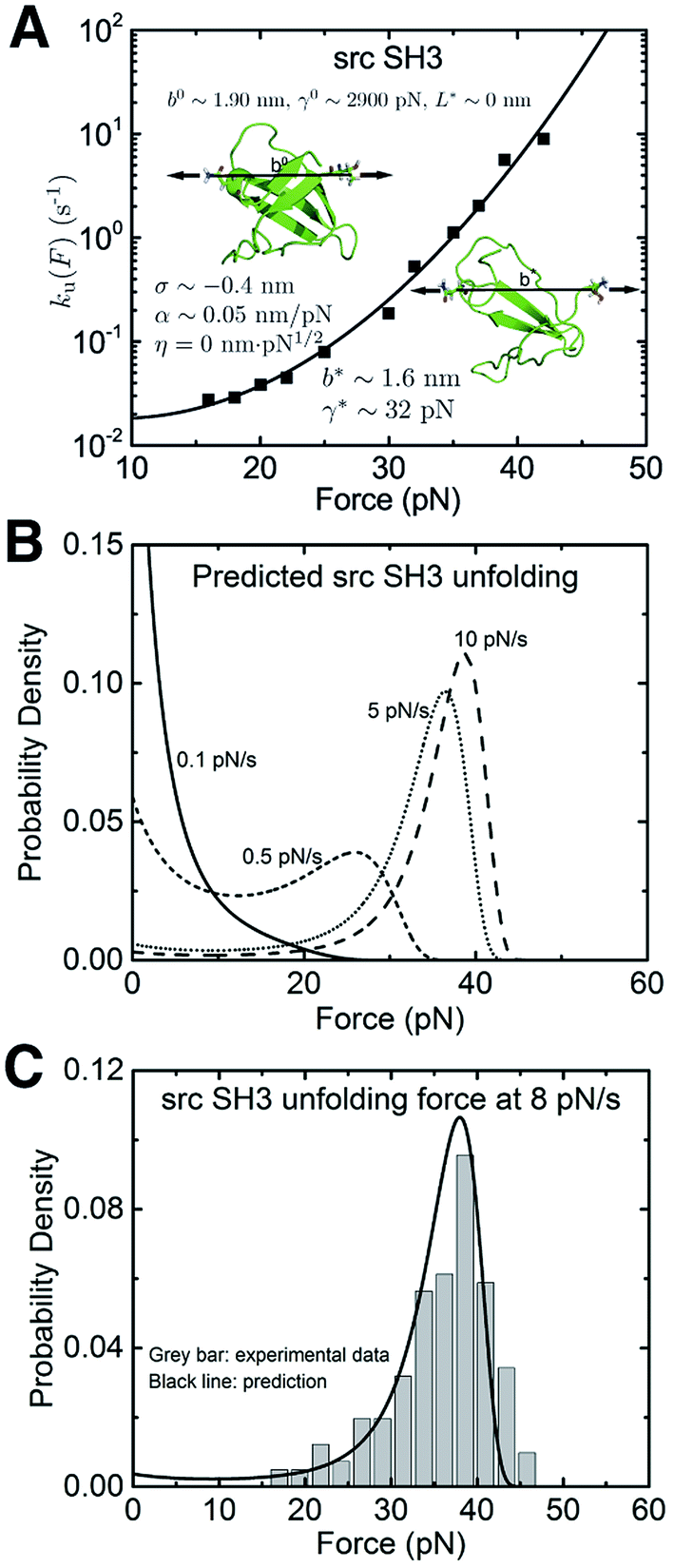 | ||
| Fig. 5 Application of eqn (5) to interpret the experimental data of src SH3: (A) The ku(F) data obtained for src SH3 (Fig. 3A in ref. 4) are indicated with black squares and fitted with eqn (5) (black line). The goodness-of-fit was evaluated using a R-square of ∼0.992 and a root mean squared error (RMSE) of ∼0.224. The best-fitting model parameters and the structural–elastic parameters determined based on the native state structure and steered MD simulations, or solved from the best-fitting parameters are indicated in the panel. (B) This panel shows the predicted src SH3 unfolding force density function p(F) using eqn (10) based on the best-fitting parameters for ku(F), at different loading rates of 0.1 pN s−1 (solid line), 0.5 pN s−1 (short dash line), 5 pN s−1 (short dot line) and 10 pN s−1 (dash line). (C) The predicted p(F) of src SH3 (solid black curve) agrees with the previously published experimental data (Fig. 2B in ref. 4) (grey bars) at a loading rate of 8 pN s−1. | ||
In order to further obtain more accurate structural–elastic properties of the transition state of the src SH3 domain, additional information on the peptide length in the transition state is needed. A previous study estimated a small transition distance of ∼0.45 nm in the force range of 15–25 pN,4 suggesting an insignificant fraction of the peptide in the transition state (ESI: SIX†). Consistently, our steered MD simulations show negligible production of the peptide under force during transition (ESI: Fig. S4†). Based on these pieces of information, we estimated b* and γ* by approximating η ∼ 0. The resulting best-fitting parameters are determined as u,0 = 0.03 ± 0.04 s−1, with 95% confidence bounds of (−0.03, 0.09) s−1; σ = −0.4 ± 0.2 nm, with 95% confidence bounds of (−1.1, 0.2) nm; and α = 0.05 ± 0.01 nm pN−1, with 95% confidence bounds of (0.03, 0.07) nm pN−1. The errors and the robustness of the parameter convergence are generated/tested similar to the case of I27 (ESI: SVI and SVII, Tables S4 and S7†).
The structural–elastic parameters of the native state are determined to be b0 ∼ 1.90 nm and γ0 ∼ 2900 pN based on the structure and steered MD simulations (ESI: SI and SII, Fig. S4 and S7†). Finally, based on the best-fitting values, b* = 1.6 ± 0.2 nm and γ* = 32 ± 9 pN are solved. The estimated value of γ* is reasonably in agreement with the value estimated based on steered MD simulations for the transition state of src SH3 (ESI: Fig. S7†).
The predicted p(F) data for src SH3 using eqn (10) at several loading rates from 0.1 pN s−1 to 10 pN s−1 are shown in Fig. 5B. The unfolding force histogram of SH3 was measured at a loading rate of 8 pN s−1,4 which is converted to a probability density function. The comparison between the experimental data and p(F) predicted with eqn (10) using the best-fitting parameters reported in this study shows very good agreement (Fig. 5C).
As shown in the previous paragraphs, the five structural–elastic parameters (b0, γ0, b*, γ*, and L*) for I27, monomeric PSGL-1/P-selectin and src SH3 are determined based on the best-fitting model parameters (σ, α, and η), molecular structures and steered MD simulations. With these structural–elastic parameters, the force-dependent transition distance  and the change of the free energy barrier
  can be computed using eqn (2) and (3) (Fig. 6). The results reveal that the three molecules have markedly different profiles of
  and
and  . For all three molecules, the complex shapes of
  over 1–100 pN force range deviate from Bell's model which assumes a force-independent transition distance. These complex profiles of
  result in complex force-dependent changes of the free energy barrier
  , which in turn affects the force-dependence of the transition rate in a very complex manner. For I27 and PSGL-1/P-selectin, the transition distances can become negative over a broad force range of up to ∼20 pN, which results in a “catch-bond” behaviour at forces below 20 pN. Remarkably, the force-dependent transition distance dramatically drops when the force increases from 0 pN to a few pN. These behaviours of the force-dependent transition distance are a result from the highly flexible nature of the peptide chain produced in the transition state.
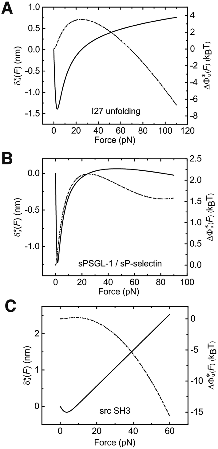 | ||
Fig. 6 Force-dependent transition distance and change of free energy barrier: The force-dependent transition distance  (solid line) calculated with eqn (2) and the force-dependent change of the free energy barrier (solid line) calculated with eqn (2) and the force-dependent change of the free energy barrier  (dash dot line) calculated with eqn (3) for I27 (A), monomeric PSGL-1/P-selectin (B) and src SH3 (C) are shown. (dash dot line) calculated with eqn (3) for I27 (A), monomeric PSGL-1/P-selectin (B) and src SH3 (C) are shown.  and and  are calculated based on the values of the five structural–elastic parameters (b0, γ0, b*, γ*, and L*) determined based on the best-fitting parameters (σ, α, and η), molecular structures and steered MD simulations for the respective molecules described in the Results section. are calculated based on the values of the five structural–elastic parameters (b0, γ0, b*, γ*, and L*) determined based on the best-fitting parameters (σ, α, and η), molecular structures and steered MD simulations for the respective molecules described in the Results section. | ||
3 Discussion
In summary, we have derived novel analytical expressions of k(F) for both the force-dependent unfolding/dissociation rate (eqn (4) and (5)) and refolding transition rate (eqn (9)) that involve overcoming a single energy barrier. The derivations are based on the structural–elastic properties of the molecule in the initial state structure and the transition state structure. As an important result, the values of the model parameters, which can be determined by fitting to experimental data, are directly related to the structural–elastic properties.In the case of unfolding/dissociation transition where the initial state is the natively folded structure, we show that application of eqn (5) does not require any prior knowledge of the structural–elastic properties of the molecule. In our previous publication, based on the prior knowledge of the crystal structure of the native state of I27 (PDB ID: 1TIT) and the structure of its transition state suggested from MD simulations,21–23 we showed that k(F) of I27 can be understood by the force-dependent extension difference between the transition state and the native state in the framework of the Arrhenius law.2 The new theory described in this paper differs from the previous work since it does not require any prior knowledge of the structural–elastic properties of molecules, making it capable of being applied to explain a wide scope of experimental data. As demonstrated in the paper, the best-fitting parameters (σ, α and η) reflect differences in the structural–elastic properties of the molecule between its transition and native states. Importantly, with additional knowledge on the structural–elastic properties of the native state that can often be obtained from the crystal structure and MD simulations, the structural–elastic parameters of the transition state structure (L*, b*, and γ*) can be solved from these best-fitting parameters.
In the case of refolding transition where the initial state structure is typically a denatured polymer, because the force-dependent deformation of the rigid core in the transition state can be ignored at low forces, a very simple expression of k(F) is obtained (eqn (9)). Fitting to experimental data can directly determine the relaxed length b* of the folded core in the transition state and the difference between the contour length of the polymer in the initial denatured state and that of the polymer produced in the transition state (L0 − L*). Because L0 is typically known, this leads to determination of b* and L* of the transition state.
In most of the experiments, k(F) is measured over a certain force range. By fitting to the data based on any kinetic model, it is attempting to extrapolate the fitted k(F) to forces beyond the experimentally measured range. However, it is dangerous if the force to which it is extrapolated is far away from the experimentally measured range. This is because the nature of the transition may vary with the force, while most of the models,9–12 including ours, are derived based on assuming a unique initial state structure and a single transition barrier. Such an assumption may only be valid in a limited force range. For example, previous AFM experiments and MD simulations22,38 suggest that at forces below 100 pN, the initial folded state of I27 has all seven β-strands folded in the native structure. However, at forces >100 pN, the initial folded state transits to an intermediate state with the A strand being detached from the B strand.22,38 Therefore, k(F) fitted based on experimental data at forces below 100 pN should not be extrapolated to forces above 100 pN and vice versa.
The simple expression of eqn (5) for unfolding/dissociation transition is derived based on large force asymptotic expansion (F ≫ kBT/b0, F ≫ kBT/b* and F ≫ kBT/A). The typical sizes of the protein domain and the folded core in the transition state are in the order of a few nanometers; therefore, kBT/b0 and kBT/b* are close to 1 pN. If in the transition state a protein peptide or a ssDNA/ssRNA polymer is produced, due to its very small bending persistence of A ∼ 1 nm,34,36kBT/A ∼ 5 pN becomes the predominating factor that imposes a restriction on the lower boundary of the force range to apply eqn (5). In actual applications, the applicable forces do not have to be much greater than 5 pN, since the force–extension curve of a flexible polymer with A ∼ 1 nm calculated based on the asymptotic large force expansion differs from the one according to the full Marko–Siggia formula30 by less than 10% at forces above 3 pN (ESI: Fig. S9†). Therefore, eqn (5) can be applied to forces >3 pN. Consistently, we have shown that eqn (5) can be applied to fit three different experimental data in this force range.
In cases where (b0 and γ0) are known from the crystal structure and MD simulations, and as a result (b*, γ* and L*) can be solved from the best-fitting values of (σ, α and η), extrapolation to lower forces is possible using the complete solution of eqn (4). In addition, since eqn (5) for unfolding/dissociation transition is not applicable at forces <3 pN, u,0 should not be interpreted as the transition rate at zero force. A better quantity that is more indicative of the zero force transition rate is ku,0 in eqn (4), which is related to u,0 according to eqn (6). If the parameters (b0, γ0, b*, and γ*) are determined, ku,0 can be estimated by applying eqn (6). However, caution should be taken for extrapolation to a low force according to eqn (4) or estimation of ku,0 according to eqn (6), since at very low forces the WLC model of the flexible protein peptide or ssDNA/ssRNA may no longer be valid due to potential formation of secondary structures on these polymers.
The effects of the elastic properties of molecules on the force-dependent unfolding/dissociation transition rate have been discussed in several previous studies.43,44 In particular, in a pioneering study published by Dembo et al.,43 by treating the native and transition states as molecular springs with different mechanical stiffness and lengths, the authors were able to predict the existence of catch, slip and ideal bonds. However, this model is too simple to explain complex ku(F) such as the “catch-to-slip” behaviour. In addition, treating the native and transition states as molecular springs makes it impossible to relate the force dependence of the transition rate to the actual structural parameters of the molecules in the native and transition states. In another work by Cossio et al.,12 the authors discussed a free energy landscape that has a force-dependent transition distance, based on which ku(F) was derived by applying Kramers kinetic theory. A phenomenological form of the force-dependent transition distance is proposed to describe the kinetic ductility that results in a monotonically decreased transition distance as a function of force, which could only describe transition with “slip” kinetics. Different from these previous studies, our derivation is based on the structural–elastic properties of molecules in their transition state and native state. Therefore, their force dependence can be much richer. Depending on the structural–elastic properties of molecules, the resulting force-dependent transition distance can be an increasing, a decreasing or a non-monotonic function of force.
The analytical expressions of k(F) (eqn (4), (5) and (9)) are derived by applying the Arrhenius law based on the structural–elastic parameters of molecules. The resulting relationship between the rate and the force-dependent transition distance,  , is identical to that obtained in the framework of Kramers theory.20 However, they differ from each other in a key aspect: in our theory δ*(F) is calculated based on the structural–elastic parameters of molecules; therefore it does not involve describing the system using any transition coordinate, and it does not depend on the dimensionality of the system. In contrast, in the framework of Kramers theory, δ*(F) has to be calculated based on a presumed one-dimensional free energy landscape that must be expressed by the extension change as the transition coordinate. As a result, δ*(F) depends on the structural–elastic parameters of molecules in our theory, while it relies on the parameters associated with the shapes of the presumed one-dimension free energy landscape in the framework of Kramers theory.20 Owing to this difference, our theory can be applied to a broader scope of experimental cases. The molecules selected to test the application of k(F) derived in this work have markedly different profiles. The fact that the expression of k(F) is able to perfectly fit the experimental data for all the molecules reveals an exquisite interplay between the structural–elastic properties of molecules and the force-dependent transition rate.
4 Methods
4.1 DNA unzipping and rezipping experiments
The DNA hairpin with the sequence of GAGTCAACGTCTGGATTTTTTTTTTTTTTTTCCAGACGTTGACTC which spanned between two dsDNA handles was tethered between a coverslip and a 2.8 μm-diameter paramagnetic bead. The force was applied through a pair of permanent magnets. The details of the force application, force calibration and loading rate control are described in our recent review paper.45 The hairpin was ligated with 5′-thiol labelled 489 bp and 5′-biotin labelled 601 bp dsDNA as described previously.31,46 DNA unzipping experiments were carried out in a buffer composed of 10 mM Tris–HCl (pH 8.0), and 100 mM KCl at a room temperature of 22 ± 1 °C.4.2 Titin I27 domain unfolding experiments
A vertical magnetic tweezer setup47 was used for conducting in vitro titin I27 domain stretching experiments. The sample protein (8I27) was designed with eight repeats of titin I27 domains spaced with flexible linkers (GGGSG) between each domain; the 8I27 was labeled with biotin-avi-tag at the N-terminus and spy-tag at the C-terminus. The expression plasmid for the sample protein was synthesised by geneArt. In a flow channel, the C-terminus of the protein was attached to the spycatcher-coated bottom surface through specific spy–spycatcher interactions, while the N-terminus was attached to a streptavidin-coated paramagnetic bead (2.8 μm in diameter, Dynabeads M-270) through specific biotin–streptavidin interactions. During experiments, the force on a single protein tether was linearly increased from ∼1 pN up to ∼120 pN with a loading rate of ∼0.08 pN s−1, to allow the unfolding of each I27 domain; after unfolding of the domains, the force was decreased to ∼1 pN for ∼60 s to allow refolding of the domains before next force-increase scans. Each I27 unfolding event and its corresponding unfolding force were detected by a home-written step-finding algorithm. All experiments were performed in buffered solution containing 1× PBS, 1% BSA, and 1 mM DTT at 22 ± 1 °C. Additional information on the step-finding algorithm, protein sequences, protein expression, and flow channel preparation can be found in previous publications.2,6,474.3 MD simulations
The all-atom molecular dynamics (MD) simulations used to estimate the value of γ of the folded structure are introduced in the ESI (SI and SII).†4.4 Data extraction
The data of k(F) for the monomeric PSGL-1/P-selectin complex and src SH3 domain, and the histogram of the unfolding force for src SH3 were obtained by digitizing previously published experimental data (Fig. 4b in ref. 3 for PSGL-1/P-selectin data, and Fig. 3A and 2B in ref. 4 for src SH3 data). The values of k(F) and the histogram of the unfolding force were extracted using ImageJ with the Figure Calibration plugin developed by Frederic V. Hessman from Institut für Astrophysik Göttingen.Author contributions
J. Y., S. G. and H. C. developed the theory. Q. T. performed steered MD simulations. S. G. and M. Y. performed the calculations and data fitting. H. Y. performed the DNA hairpin unzipping and rezipping experiments. Q. T. and S. L. performed the titin I27 domain unfolding experiments. J. Y. and S. G. wrote the paper. J. Y. conceived and supervised the study.Conflicts of interest
There is no conflicts to declare.Acknowledgements
The authors thank Jacques Prost (Institut Curie) for many stimulating discussions. Work done in Singapore is supported by the National Research Foundation (NRF), Prime Minister's Office, Singapore under its NRF Investigatorship Programme (NRF Investigatorship Award No. NRF-NRFI2016-03), Singapore Ministry of Education Academic Research Fund Tier 3 (MOE2016-T3-1-002), and the Human Frontier Science Program (RGP00001/2016) [to J. Y.]. Work done in China is supported by the National Natural Science Foundation of China (11474237) [to H. C.].Notes and references
- T. Iskratsch, H. Wolfenson and M. P. Sheetz, Nat. Rev. Mol. Cell Biol., 2014, 15, 825–833 CrossRef PubMed
.
- G. Yuan, S. Le, M. Yao, H. Qian, X. Zhou, J. Yan and H. Chen, Angew. Chem., 2017, 129, 5582–5585 CrossRef
- B. T. Marshall, M. Long, J. W. Piper, T. Yago, R. P. McEver and C. Zhu, Nature, 2003, 423, 190–193 CrossRef PubMed
- B. Jagannathan, P. J. Elms, C. Bustamante and S. Marqusee, Proc. Natl. Acad. Sci. U. S. A., 2012, 109, 17820–17825 CrossRef PubMed
- S. Rakshit, Y. Zhang, K. Manibog, O. Shafraz and S. Sivasankar, Proc. Natl. Acad. Sci. U. S. A., 2012, 109, 18815–18820 CrossRef PubMed
- H. Chen, G. Yuan, R. S. Winardhi, M. Yao, I. Popa, J. M. Fernandez and J. Yan, J. Am. Chem. Soc., 2015, 137, 3540–3546 CrossRef PubMed
- D. T. Edwards, J. K. Faulk, A. W. Sanders, M. S. Bull, R. Walder, M.-A. LeBlanc, M. C. Sousa and T. T. Perkins, Nano Lett., 2015, 15, 7091–7098 CrossRef PubMed
- G. Bell, Science, 1978, 200, 618–627 Search PubMed
- G. Hummer and A. Szabo, Biophys. J., 2003, 85, 5–15 CrossRef PubMed
- E. Evans and K. Ritchie, Biophys. J., 1997, 72, 1541–1555 CrossRef PubMed
- O. K. Dudko, G. Hummer and A. Szabo, Phys. Rev. Lett., 2006, 96, 108101 CrossRef PubMed
- P. Cossio, G. Hummer and A. Szabo, Biophys. J., 2016, 111, 832–840 CrossRef PubMed
- Y. V. Pereverzev, O. V. Prezhdo, M. Forero, E. V. Sokurenko and W. E. Thomas, Biophys. J., 2005, 89, 1446–1454 CrossRef PubMed
- V. Barsegov and D. Thirumalai, Proc. Natl. Acad. Sci. U. S. A., 2005, 102, 1835–1839 CrossRef PubMed
- E. Evans, A. Leung, V. Heinrich and C. Zhu, Proc. Natl. Acad. Sci. U. S. A., 2004, 101, 11281–11286 CrossRef PubMed
- C. A. Pierse and O. K. Dudko, Phys. Rev. Lett., 2017, 118, 088101 CrossRef PubMed
- D. Bartolo, I. Derényi and A. Ajdari, Phys. Rev. E: Stat., Nonlinear, Soft Matter Phys., 2002, 65, 051910 CrossRef PubMed
- A. A. Rebane, L. Ma and Y. Zhang, Biophys. J., 2016, 110, 441–454 CrossRef PubMed
- H. A. Kramers, Physica, 1940, 7, 284–304 CrossRef
- O. K. Dudko, G. Hummer and A. Szabo, Proc. Natl. Acad. Sci. U. S. A., 2008, 105, 15755–15760 CrossRef PubMed
- H. Lu, B. Isralewitz, A. Krammer, V. Vogel and K. Schulten, Biophys. J., 1998, 75, 662–671 CrossRef PubMed
- H. Lu and K. Schulten, Chem. Phys., 1999, 247, 141–153 CrossRef
- R. B. Best, S. B. Fowler, J. L. Herrera, A. Steward, E. Paci and J. Clarke, J. Mol. Biol., 2003, 330, 867–877 CrossRef PubMed
- P. M. Williams, S. B. Fowler, R. B. Best, J. L. Toca-Herrera, K. A. Scott, A. Steward and J. Clarke, Nature, 2003, 422, 446–449 CrossRef PubMed
- C. Bouchiat, M. Wang, J.-F. Allemand, T. Strick, S. Block and V. Croquette, Biophys. J., 1999, 76, 409–413 CrossRef PubMed
- P. Cong, L. Dai, H. Chen, J. R. van der Maarel, P. S. Doyle and J. Yan, Biophys. J., 2015, 109, 2338–2351 CrossRef PubMed
- S. Cocco, J. Yan, J.-F. Léger, D. Chatenay and J. F. Marko, Phys. Rev. E: Stat., Nonlinear, Soft Matter Phys., 2004, 70, 011910 CrossRef PubMed
- I. Rouzina and V. A. Bloomfield, Biophys. J., 2001, 80, 882–893 CrossRef PubMed
- S. B. Smith, Y. Cui and C. Bustamente, Science, 1996, 271, 795 CrossRef PubMed
- J. Marko and E. Siggia, Macromolecules, 1995, 28, 8759–8770 CrossRef
- H. You, X. Zeng, Y. Xu, C. J. Lim, A. K. Efremov, A. T. Phan and J. Yan, Nucleic Acids Res., 2014, 42, 8789–8795 CrossRef PubMed
- M. Yao, B. T. Goult, B. Klapholz, X. Hu, C. P. Toseland, Y. Guo, P. Cong, M. P. Sheetz and J. Yan, Nat. Commun., 2016, 7, 11966 CrossRef PubMed
- S. Le, X. Hu, M. Yao, H. Chen, M. Yu, X. Xu, N. Nakazawa, F. M. Margadant, M. P. Sheetz and J. Yan, Cell Rep., 2017, 21, 2714–2723 CrossRef PubMed
- A. Bosco, J. Camunas-Soler and F. Ritort, Nucleic Acids Res., 2013, 42, 2064–2074 CrossRef PubMed
- H. You, S. Guo, S. Le, Q. Tang, M. Yao, X. Zhao and J. Yan, J. Phys. Chem. Lett., 2018, 9, 811–816 CrossRef PubMed
- R. S. Winardhi, Q. Tang, J. Chen, M. Yao and J. Yan, Biophys. J., 2016, 111, 2349–2357 CrossRef PubMed
- M. Carrion-Vazquez, A. F. Oberhauser, S. B. Fowler, P. E. Marszalek, S. E. Broedel, J. Clarke and J. M. Fernandez, Proc. Natl. Acad. Sci. U. S. A., 1999, 96, 3694–3699 CrossRef
- P. E. Marszalek, H. Lu, H. Li, M. Carrion-Vazquez, A. F. Oberhauser, K. Schulten and J. M. Fernandez, Nature, 1999, 402, 100–103 CrossRef PubMed
- W. S. Somers, J. Tang, G. D. Shaw and R. T. Camphausen, Cell, 2000, 103, 467–479 CrossRef PubMed
- K. Konstantopoulos, W. D. Hanley and D. Wirtz, Curr. Biol., 2003, 13, R611–R613 CrossRef PubMed
- J. Lou, T. Yago, A. G. Klopocki, P. Mehta, W. Chen, V. I. Zarnitsyna, N. V. Bovin, C. Zhu and R. P. McEver, J. Cell Biol., 2006, 174, 1107–1117 CrossRef PubMed
- J. Lou and C. Zhu, Biophys. J., 2007, 92, 1471–1485 CrossRef PubMed
- M. Dembo, D. Torney, K. Saxman and D. Hammer, Proc. R. Soc. Lond. B Biol. Sci., 1988, 234, 55–83 CrossRef
- J. Valle-Orero, E. C. Eckels, G. Stirnemann, I. Popa, R. Berkovich and J. M. Fernandez, Biochem. Biophys. Res. Commun., 2015, 460, 434–438 CrossRef PubMed
- X. Zhao, X. Zeng, C. Lu and J. Yan, Nanotechnology, 2017, 28, 414002 CrossRef PubMed
- H. You, J. Wu, F. Shao and J. Yan, J. Am. Chem. Soc., 2015, 137, 2424–2427 CrossRef PubMed
- H. Chen, H. Fu, X. Zhu, P. Cong, F. Nakamura and J. Yan, Biophys. J., 2011, 100, 517–523 CrossRef PubMed
Footnotes |
| † Electronic supplementary information (ESI) available. See DOI: 10.1039/c8sc01319e |
| ‡ These authors contributed equally to this work. |
| This journal is © The Royal Society of Chemistry 2018 |