 Open Access Article
MoleculeNet: a benchmark for molecular machine learning†
Zhenqin
Wu‡
 a,
Bharath
Ramsundar‡
b,
Evan N.
Feinberg§
c,
Joseph
Gomes§
 a,
Caleb
Geniesse
c,
Aneesh S.
Pappu
b,
Karl
Leswing
d and
Vijay
Pande
*a
aDepartment of Chemistry, Stanford University, Stanford, CA 94305, USA. E-mail: pande@stanford.edu
bDepartment of Computer Science, Stanford University, Stanford, CA 94305, USA
cProgram in Biophysics, Stanford School of Medicine, Stanford, CA 94305, USA
dSchrodinger Inc., USA
First published on 31st October 2017
Abstract
Molecular machine learning has been maturing rapidly over the last few years. Improved methods and the presence of larger datasets have enabled machine learning algorithms to make increasingly accurate predictions about molecular properties. However, algorithmic progress has been limited due to the lack of a standard benchmark to compare the efficacy of proposed methods; most new algorithms are benchmarked on different datasets making it challenging to gauge the quality of proposed methods. This work introduces MoleculeNet, a large scale benchmark for molecular machine learning. MoleculeNet curates multiple public datasets, establishes metrics for evaluation, and offers high quality open-source implementations of multiple previously proposed molecular featurization and learning algorithms (released as part of the DeepChem open source library). MoleculeNet benchmarks demonstrate that learnable representations are powerful tools for molecular machine learning and broadly offer the best performance. However, this result comes with caveats. Learnable representations still struggle to deal with complex tasks under data scarcity and highly imbalanced classification. For quantum mechanical and biophysical datasets, the use of physics-aware featurizations can be more important than choice of particular learning algorithm.
1 Introduction
Overlap between chemistry and statistical learning has had a long history. The field of cheminformatics has been utilizing machine learning methods in chemical modeling (e.g. quantitative structure activity relationships, QSAR) for decades.1–6 In the recent 10 years, with the advent of sophisticated deep learning methods,7,8 machine learning has gathered increasing amounts of attention from the scientific community. Data-driven analysis has become a routine step in many chemical and biological applications, including virtual screening,9–12 chemical property prediction,13–16 and quantum chemistry calculations.17–20In many such applications, machine learning has shown strong potential to compete with or even outperform conventional ab initio computations.16,18 It follows that introduction of novel machine learning methods has the potential to reshape research on properties of molecules. However, this potential has been limited by the lack of a standard evaluation platform for proposed machine learning algorithms. Algorithmic papers often benchmark proposed methods on disjoint dataset collections, making it a challenge to gauge whether a proposed technique does in fact improve performance.
Data for molecule-based machine learning tasks are highly heterogeneous and expensive to gather. Obtaining precise and accurate results for chemical properties typically requires specialized instruments as well as expert supervision (contrast with computer speech and vision, where lightly trained workers can annotate data suitable for machine learning systems). As a result, molecular datasets are usually much smaller than those available for other machine learning tasks. Furthermore, the breadth of chemical research means our interests with respect to a molecule may range from quantum characteristics to measured impacts on the human body. Molecular machine learning methods have to be capable of learning to predict this very broad range of properties. Complicating this challenge, input molecules can have arbitrary size and components, highly variable connectivity and many three dimensional conformers (three dimensional molecular shapes). To transform molecules into a form suitable for conventional machine learning algorithms (that usually accept fixed length input), we have to extract useful and related information from a molecule into a fixed dimensional representation (a process called featurization).21–23
To put it simply, building machine learning models on molecules requires overcoming several key issues: limited amounts of data, wide ranges of outputs to predict, large heterogeneity in input molecular structures and appropriate learning algorithms. Therefore, this work aims to facilitate the development of molecular machine learning methods by curating a number of dataset collections, creating a suite of software that implements many known featurizations of molecules, and providing high quality implementations of many previously proposed algorithms. Following the footsteps of WordNet24 and ImageNet,25 we call our suite MoleculeNet, a benchmark collection for molecular machine learning.
In machine learning, a benchmark serves as more than a simple collection of data and methods. The introduction of the ImageNet benchmark in 2009 has triggered a series of breakthroughs in computer vision, and in particular has facilitated the rapid development of deep convolutional networks. The ILSVRC, an annual contest held by the ImageNet team,26 draws considerable attention from the community, and greatly stimulates collaborations and competitions across the field. The contest has given rise to a series of prominent machine learning models such as AlexNet,27 GoogLeNet,28 ResNet29 which have had broad impact on the academic and industrial computer science communities. We hope that MoleculeNet will trigger similar breakthroughs by serving as a platform for the wider community to develop and improve models for learning molecular properties.
In particular, MoleculeNet contains data on the properties of over 700![[thin space (1/6-em)]](https://www.rsc.org/images/entities/char_2009.gif) 000 compounds. All datasets have been curated and integrated into the open source DeepChem package.30 Users of DeepChem can easily load all MoleculeNet benchmark data through provided library calls. MoleculeNet also contributes high quality implementations of well known (bio)chemical featurization methods. To facilitate comparison and development of new methods, we also provide high quality implementations of several previously proposed machine learning methods. Our implementations are integrated with DeepChem, and depend on Scikit-Learn31 and Tensorflow32 underneath the hood. Finally, evaluation of machine learning algorithms requires defined methods to split datasets into training/validation/test collections. Random splitting, common in machine learning, is often not correct for chemical data.33 MoleculeNet contributes a library of splitting mechanisms to DeepChem and evaluates all algorithms with multiple choices of data split. MoleculeNet provide a series of benchmark results of implemented machine learning algorithms using various featurizations and splits upon our dataset collections. These results are provided within this paper, and will be maintained online in an ongoing fashion as part of DeepChem.
000 compounds. All datasets have been curated and integrated into the open source DeepChem package.30 Users of DeepChem can easily load all MoleculeNet benchmark data through provided library calls. MoleculeNet also contributes high quality implementations of well known (bio)chemical featurization methods. To facilitate comparison and development of new methods, we also provide high quality implementations of several previously proposed machine learning methods. Our implementations are integrated with DeepChem, and depend on Scikit-Learn31 and Tensorflow32 underneath the hood. Finally, evaluation of machine learning algorithms requires defined methods to split datasets into training/validation/test collections. Random splitting, common in machine learning, is often not correct for chemical data.33 MoleculeNet contributes a library of splitting mechanisms to DeepChem and evaluates all algorithms with multiple choices of data split. MoleculeNet provide a series of benchmark results of implemented machine learning algorithms using various featurizations and splits upon our dataset collections. These results are provided within this paper, and will be maintained online in an ongoing fashion as part of DeepChem.
The related work section will review prior work in the chemistry community on gathering curated datasets and discuss how MoleculeNet differs from these previous efforts. The methods section reviews the dataset collections, metrics, featurization methods, and machine learning models included as part of MoleculeNet. The results section will analyze the benchmarking results to draw conclusions about the algorithms and datasets considered.
2 Related work
MoleculeNet draws upon a broader movement within the chemical community to gather large sources of curated data. PubChem34 and PubChem BioAssasy35 gather together thousands of bioassay results, along with millions of unique molecules tested within these assays. The ChEMBL database offers a similar service, with millions of bioactivity outcomes across thousands of protein targets. Both PubChem and ChEMBL are human researcher oriented, with web portals that facilitate browsing of the available targets and compounds. ChemSpider is a repository of nearly 60 million chemical structures, with web based search capabilities for users. The Crystallography Open Database36 and Cambridge Structural Database37 offer large repositories of organic and inorganic compounds. The protein data bank38 offers a repository of experimentally resolved three dimensional protein structures. This listing is by no means comprehensive; the methods section will discuss a number of smaller data sources in greater detail.These past efforts have been critical in enabling the growth of computational chemistry. However, these previous databases are not machine-learning focused. In particular, these collections don't define metrics which measure the effectiveness of algorithmic methods in understanding the data contained. Furthermore, there is no prescribed separation of the data into training/validation/test sets (critical for machine learning development). Without specified metrics or splits, the choice is left to individual researchers, and there are indeed many chemical machine learning papers which use subsets of these data stores for machine learning evaluation. Unfortunately, the choice of metric and subset varies widely between groups, so two methods papers using PubChem data may be entirely incomparable. MoleculeNet aims to bridge this gap by providing benchmark results for a reasonable range of metrics, splits, and subsets of these (and other) data collections.
It's important to note that there have been some efforts to create benchmarking datasets for machine learning in chemistry. The Quantum Machine group39 and previous work on multitask learning10 both introduce benchmarking collections which have been used in multiple papers. MoleculeNet incorporates data from both these efforts and significantly expands upon them.
3 Methods
MoleculeNet is based on the open source package DeepChem.30Fig. 1 shows an annotated DeepChem benchmark script. Note how different choices for data splitting, featurization, and model are available. DeepChem also directly provides molnet sub-module to support benchmarking. The single line below runs benchmarking on the specified dataset, model and featurizer. User defined models capable of handling DeepChem datasets are also supported.| deepchem.molnet.run_benchmark (datasets, model, split, featurizer) |
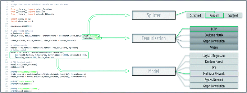 | ||
| Fig. 1 Example code for benchmark evaluation with DeepChem, multiple methods are provided for data splitting, featurization and learning. | ||
In this section, we will further elaborate the benchmarking system, introducing available datasets as well as implemented splitting, metrics, featurization, and learning methods.
3.1 Datasets
MoleculeNet is built upon multiple public databases. The full collection currently includes over 700![[thin space (1/6-em)]](https://www.rsc.org/images/entities/char_2009.gif) 000 compounds tested on a range of different properties. These properties can be subdivided into four categories: quantum mechanics, physical chemistry, biophysics and physiology. As illustrated in Fig. 2, separate datasets in the MoleculeNet collection cover various levels of molecular properties, ranging from molecular-level properties to macroscopic influences on human body. For each dataset, we propose a metric and a splitting pattern (introduced in the following texts) that best fit the properties of the dataset. Performances on the recommended metric and split are reported in the results section.
000 compounds tested on a range of different properties. These properties can be subdivided into four categories: quantum mechanics, physical chemistry, biophysics and physiology. As illustrated in Fig. 2, separate datasets in the MoleculeNet collection cover various levels of molecular properties, ranging from molecular-level properties to macroscopic influences on human body. For each dataset, we propose a metric and a splitting pattern (introduced in the following texts) that best fit the properties of the dataset. Performances on the recommended metric and split are reported in the results section.
In most datasets, SMILES strings40 are used to represent input molecules, 3D coordinates are also included in part of the collection as molecular features, which enables different methods to be applied. Properties, or output labels, are either 0/1 for classification tasks, or floating point numbers for regression tasks. At the time of writing, MoleculeNet contains 17 datasets prepared and benchmarked, but we anticipate adding further datasets in an on-going fashion. We also highly welcome contributions from other public data collections. For more detailed dataset structure requirements and instructions on curating datasets, please refer to the tutorial notebook in the example folder of DeepChem github repository.
Table 1 lists details of datasets in the collection, including tasks, compounds and their features, recommended splits and metrics. Contents of each dataset will be elaborated in this subsection, function calls to access the datasets can be found in the ESI.†
| Category | Dataset | Data type | Tasks | Compounds | Rec – split | Rec – metric | |
|---|---|---|---|---|---|---|---|
| Quantum mechanics | QM7 | SMILES, 3D coordinates | 1 | Regression | 7165 | Stratified | MAE |
| QM7b | 3D coordinates | 14 | Regression | 7211 | Random | MAE | |
| QM8 | SMILES, 3D coordinates | 12 | Regression | 21![[thin space (1/6-em)]](https://www.rsc.org/images/entities/char_2009.gif) 786 786 |
Random | MAE | |
| QM9 | SMILES, 3D coordinates | 12 | Regression | 133![[thin space (1/6-em)]](https://www.rsc.org/images/entities/char_2009.gif) 885 885 |
Random | MAE | |
| Physical chemistry | ESOL | SMILES | 1 | Regression | 1128 | Random | RMSE |
| FreeSolv | SMILES | 1 | Regression | 643 | Random | RMSE | |
| Lipophilicity | SMILES | 1 | Regression | 4200 | Random | RMSE | |
| Biophysics | PCBA | SMILES | 128 | Classification | 439![[thin space (1/6-em)]](https://www.rsc.org/images/entities/char_2009.gif) 863 863 |
Random | PRC-AUC |
| MUV | SMILES | 17 | Classification | 93![[thin space (1/6-em)]](https://www.rsc.org/images/entities/char_2009.gif) 127 127 |
Random | PRC-AUC | |
| HIV | SMILES | 1 | Classification | 41![[thin space (1/6-em)]](https://www.rsc.org/images/entities/char_2009.gif) 913 913 |
Scaffold | ROC-AUC | |
| PDBbind | SMILES, 3D coordinates | 1 | Regression | 11![[thin space (1/6-em)]](https://www.rsc.org/images/entities/char_2009.gif) 908 908 |
Time | RMSE | |
| BACE | SMILES | 1 | Classification | 1522 | Scaffold | ROC-AUC | |
| Physiology | BBBP | SMILES | 1 | Classification | 2053 | Scaffold | ROC-AUC |
| Tox21 | SMILES | 12 | Classification | 8014 | Random | ROC-AUC | |
| ToxCast | SMILES | 617 | Classification | 8615 | Random | ROC-AUC | |
| SIDER | SMILES | 27 | Classification | 1427 | Random | ROC-AUC | |
| ClinTox | SMILES | 2 | Classification | 1491 | Random | ROC-AUC |
The datasets introduced above (QM7, QM7b, QM8, QM9) were curated as part of the Quantum-Machine effort,39 which has processed a number of datasets to measure the efficacy of machine-learning methods for quantum chemistry.
![[thin space (1/6-em)]](https://www.rsc.org/images/entities/char_2009.gif) D at pH 7.4) of 4200 compounds.
D at pH 7.4) of 4200 compounds.
![[thin space (1/6-em)]](https://www.rsc.org/images/entities/char_2009.gif) 000 compounds.47 Screening results were evaluated and placed into three categories: confirmed inactive (CI), confirmed active (CA) and confirmed moderately active (CM). We further combine the latter two labels, making it a classification task between inactive (CI) and active (CA and CM). As we are more interested in discover new categories of HIV inhibitors, scaffold splitting (introduced in the next subsection) is recommended for this dataset.
000 compounds.47 Screening results were evaluated and placed into three categories: confirmed inactive (CI), confirmed active (CA) and confirmed moderately active (CM). We further combine the latter two labels, making it a classification task between inactive (CI) and active (CA and CM). As we are more interested in discover new categories of HIV inhibitors, scaffold splitting (introduced in the next subsection) is recommended for this dataset.
3.2 Dataset splitting
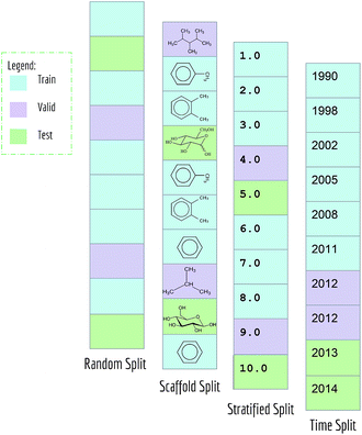
Typical machine learning methods require datasets to be split into training/validation/test subsets (or alternatively into K-folds) for benchmarking. All MoleculeNet datasets are split into training, validation and test, following a 80/10/10 ratio. Training sets were used to train models, while validation sets were used for tuning hyperparameters, and test sets were used for evaluation of models.As mentioned previously, random splitting of molecular data isn't always best for evaluating machine learning methods. Consequently, MoleculeNet implements multiple different splittings for each dataset (Fig. 3). Random splitting randomly splits samples into the training/validation/test subsets. Scaffold splitting splits the samples based on their two-dimensional structural frameworks,62 as implemented in RDKit.63 Since scaffold splitting attempts to separate structurally different molecules into different subsets, it offers a greater challenge for learning algorithms than the random split.
In addition, a stratified random sampling method is implemented on the QM7 dataset to reproduce the results from the original work.18 This method sorts datapoints in order of increasing label value (note this is only defined for real-valued output). This sorted list is then split into training/validation/test by ensuring that each set contains the full range of provided labels. Time splitting is also adopted for dataset that includes time information (PDBbind). Under this splitting method, model will be trained on older data and tested on newer data, mimicking real world development condition.
MoleculeNet contributes the code for these splitting methods into DeepChem. Users of the library can use these splits on new datasets with short library calls.
3.3 Metrics
MoleculeNet contains both regression datasets (QM7, QM7b, QM8, QM9, ESOL, FreeSolv, lipophilicity and PDBbind) and classification datasets (PCBA, MUV, HIV, BACE, BBBP, Tox21, ToxCast and SIDER). Consequently, different performance metrics need to be measured for each. Following suggestions from the community,64 regression datasets are evaluated by mean absolute error (MAE) and root-mean-square error (RMSE), classification datasets are evaluated by area under curve (AUC) of the receiver operating characteristic (ROC) curve65 and the precision recall curve (PRC).66 For datasets containing more than one task, we report the mean metric values over all tasks.To allow better comparison, we propose regression metrics according to previous work on either same models or datasets. For classification datasets, we propose recommended metrics from the two commonly used metrics: AUC-PRC and AUC-ROC. Four representative sets of ROC curves and PRCs are depicted in Fig. 4, resulting from the predictions of logistic regression and graph convolutional models on four tasks. Details about these tasks and AUC values of all curves are listed in Table 2. Note that these four tasks have different class imbalances, represented as the number of positive samples and negative samples.
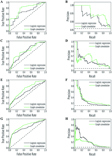 | ||
| Fig. 4 Receiver operating characteristic (ROC) curves and precision recall curves (PRC) for predictions of logistic regression and graph convolutional models under different class imbalance condition (details listed in Table 2). (A, B) task “FDA_APPROVED” from ClinTox, test subset; (C, D) task “Hepatobiliary disorders” from SIDER, test subset; (E, F) task “NR-ER” from Tox21, validation subset; (G, H): task “HIV_active” from HIV, test subset. Black dashed lines are performances of random classifiers. | ||
| Task | P/Na | Model | ROC | PRC |
|---|---|---|---|---|
| a Number of positive samples/number of negative samples. | ||||
| “FDA_APPROVED” ClinTox, test subset | 128/21 | Logistic regression | 0.691 | 0.932 |
| Graph convolution | 0.791 | 0.959 | ||
| “Hepatobiliary disorders” SIDER, test subset | 64/79 | Logistic regression | 0.659 | 0.612 |
| Graph convolution | 0.675 | 0.620 | ||
| “NR-ER” Tox21, valid subset | 81/553 | Logistic regression | 0.612 | 0.308 |
| Graph convolution | 0.705 | 0.333 | ||
| “HIV_active” HIV, test subset | 132/4059 | Logistic regression | 0.724 | 0.236 |
| Graph convolution | 0.783 | 0.169 | ||
As noted in previous literature,66 ROC curves and PRCs are highly correlated, but perform significantly differently in case of high class imbalance. As shown in Fig. 4, the fraction of positive samples decreases from over 80% (panels A and B) to less than 5% (panels G and H). This change accompanies the difference in how the two metrics treat model performances. In particular, PRCs put more emphasis on the low recall (also known as true positive rate (TPR)) side in case of highly imbalanced data: logistic regression slightly outperforms graph convolutional models in the low TPR side of ROC curves (panels C, E and G, lower left corner), which creates different margins on the low recall side of PRCs.
ROC curves and PRCs share one same axis, while using false positive rate (FPR) and precision for the other axis respectively. Recall that FPR and precision are defined as follows:
When positive samples form only a small proportion of all samples, false positive predictions exert a much greater influence on precision than FPR, amplifying the difference between PRC and ROC curves. Virtual screening experiments do have extremely low positive rates, suggesting that the correct metric to analyze may depend on the experiment at hand. In this work, we hence propose recommended metrics based on positive rates, PRC-AUC is used for datasets with positive rates less than 2%, otherwise ROC-AUC is used.
3.4 Featurization
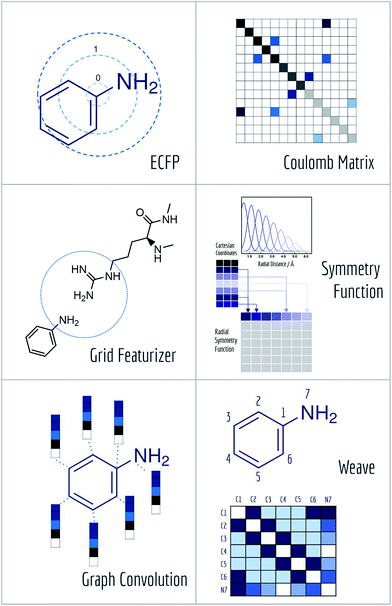
A core challenge for molecular machine learning is effectively encoding molecules into fixed-length strings or vectors. Although SMILES strings are unique representations of molecules, most molecular machine learning methods require further information to learn sophisticated electronic or topological features of molecules from limited amounts of data. (Recent work has demonstrated the ability to learn useful representations from SMILES strings using more sophisticated methods,67 so it may be feasible to use SMILES strings for further learning tasks in the near future.) Furthermore, the enormity of chemical space often requires representations of molecules specifically suited to the learning task at hand. MoleculeNet contains implementations of six useful molecular featurization methods (Fig. 5).After hashing all these substructures into a fixed length binary fingerprint, the representation contains information about topological characteristics of the molecule, which enables it to be applied to tasks such as similarity searching and activity prediction. The MoleculeNet implementation uses ECFP4 fingerprints generated by RDKit.63
Here, the off-diagonal elements correspond to the Coulomb repulsion between atoms I and J, and the diagonal elements correspond to a polynomial fit of atomic self-energy to nuclear charge. The Coulomb matrix of a molecule is invariant to translation and rotation of that molecule, but not with respect to atom index permutation. In the construction of Coulomb matrix, we first use the nuclear charges and distance matrix generated by RDKit63 to acquire the original Coulomb matrix, then an optional random atom index sorting and binary expansion transformation can be applied during training in order to achieve atom index invariance, as reported by Montavon et al.18
The grid featurizer was inspired by the NNscore featurizer68 and SPLIF69 but optimized for speed, robustness, and generalizability. The intermolecular interactions enumerated by the featurizer include salt bridges and hydrogen bonding between protein and ligand, intra-ligand circular fingerprints, intra-protein circular fingerprints, and protein–ligand SPLIF fingerprints. A more detailed breakdown can be found in the ESI.†
As symmetry function put most emphasis on spatial positions of atoms, it is intrinsically hard for it to distinguish different atom types (H, C, O). MoleculeNet utilizes a slightly modified version of original symmetry function71 which further separate radial and angular symmetry terms according to the type of atoms in the pair or triplet. Further details can be found in the article71 or our implementation.
3.5 Models – conventional models
MoleculeNet tests the performance of various machine learning models on the datasets discussed previously. These models could be further categorized into conventional method and graph-based method according to their structures and input types. The following sections will give brief introductions to benchmarked algorithms. The results section will discuss performance numbers in detail. Here we briefly review conventional methods including logistic regression, support vector classification, kernel ridge regression, random forests,72 gradient boosting,73 multitask networks,9,10 bypass networks74 and influence relevance voting.75 The next section graph-based models will give introductions to graph convolutional models,22 weave models,23 directed acyclic graph models,14 deep tensor neural networks,19 ANI-1 (ref. 71) and message passing neural networks.76 As part of this work, all methods are implemented in the open source DeepChem package.30The Jaccard–Tanimoto similarity between fingerprints of compounds is used as the similarity measurement:
Then IRV model calculates a weighted sum of labels of top K similar compounds to predict the result, in which weights are the outputs of a one-hidden layer neural network with similarities and rankings of top-K compounds as input. Detailed descriptions of the model can be found in the original article.75
3.6 Models – graph based models
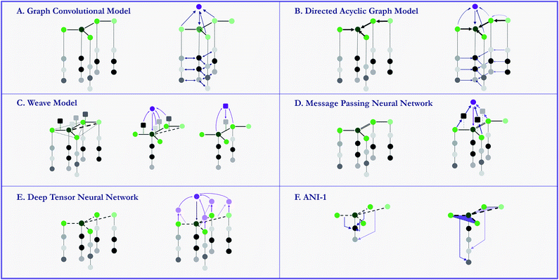
Early attempts to directly use molecular structures instead of selected features has emerged in 1990s.81,82 While in recent years, models propelled by the very similar idea start to grow rapidly. These specifically designed methods, namely graph-based models, are naturally suitable for modelling molecules. By defining atoms as nodes, bonds as edges, molecules can be modeled as mathematical graphs. As noted in a recent paper,76 this natural similarity has inspired a number of models to utilize the graph structure of molecules to gain higher performances. In general, graph-based models apply adaptive functions to nodes and edges, allowing for a learnable featurization process. MoleculeNet provides implementations of multiple graph-based models which use different variants of molecular graphs. Fig. 6 provide simple illustrations of these methods' core structures. We describe these methods in details in the following sections. To further validate the model implementations, we compare the performances of these models with their original sources, results can be found in the ESI.†On a higher level, graph convolutional models treat molecules as undirected graphs, and apply the same learnable function to every node (atom) and its neighbors (bonded atoms) in the graph. This structure recapitulates convolution layers in visual recognition deep networks.
MoleculeNet uses the graph convolutional implementation in DeepChem from previous work.56 This implementation converts SMILES strings into molecular graphs using RDKit63 As mentioned previously, the initial representations assign to each atom a vector of features including its element, connectivity, valence, etc. Then several graph convolutional modules, each consisting of a graph convolutional layer, a batch normalization layer and a graph pool layer, are sequentially added, followed by a fully-connected dense layer. Finally, the feature vectors for all nodes (atoms) are summed, generating a graph feature vector, which is fed to a classification or regression layer.
In our implementation, a molecule is first encoded into a list of atomic features and a matrix of pair features by the weave model's featurization method. Then in each weave module, these features are inputted into four sets of fully connected layers (corresponding to four paths from two original features to two updated features) and concatenated to form new atomic and pair features. After stacking several weave modules, a similar gather layer combines atomic features together to form molecular features that are fed into task-specific layers.
In the actual calculations of a graph, a vector of graph features is calculated for each atom based on its atomic features (reusing the graph convolutions featurizer) and its parents' graph features. As features gradually propagate through bonds, information converges on the central atom. Then a final sum of all graphs gives the molecular features, which are fed into classification or regression tasks. Note that na graphs are evaluated for each molecule, which can cause a significant increase in required calculations.
We reimplement the model proposed by Schütt et al.19 in a more generalized fashion. Atom numbers and a distance matrix are calculated by RDKit,63 using the Coulomb matrix featurizer. After embedding atom numbers into feature vectors ai, we update ai in each convolutional layer by adding the outputs from all network layers which use dij and aj (i ≠ j) as input. After several layers of convolutions, all atomic features are summed together to form molecular features, used for classification and regression tasks.
This model is first introduced by Smith et al.71 In their original article, the model is trained on 58k small molecules with 8 or less heavy atoms, each with multiple poses and potentials. Training set in total has 17.2 million data points, which is far bigger than qm8 or qm9 in our collection. Since we only have molecules in their most stable configuration, we cannot expect similar level of accuracy. Further comparison and benchmarking with similar size of training set is left to future work.
Here we reimplemented the best-performing model in the original article: using an Edge network as message passing function and a set2set model83 as readout function. In message passing phase, an edge-dependent neural network maps all neighbour atoms' feature vectors to updating messages, which are then merged using gated recurrent units. In the final readout phase, feature vectors for all atoms are regarded as a set, then an LSTM using attention mechanism is applied on the set for multiple steps, with its final state used as the output for the molecule.
4 Results and discussion
In this section, we discuss the performance of benchmarked models on MoleculeNet datasets. Different models are applied depending on the size, features and task types of the dataset. All graph models use their corresponding featurizations. Non-graph models use ECFP featurizations by default, Coulomb Matrix (CM) and Grid featurizer are also applied for certain datasets.We run a brief Gaussian process hyperparameter optimization on each combination of dataset and model. Then three independent runs with different random seeds are performed. More detailed description of optimization method and performance tables can be found in ESI.† Note that all benchmark results presented here are the average of three runs, with standard deviations listed or illustrated as error bars.
We also run a set of experiments focusing on how variable size of training set affect model performances (Tox21, FreeSolv and QM7). Details will be presented in the following texts.
4.1 Biophysics and physiology tasks
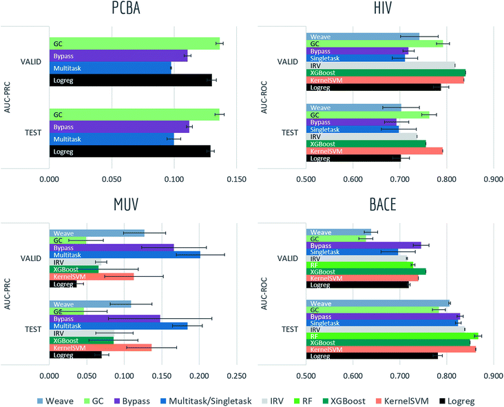
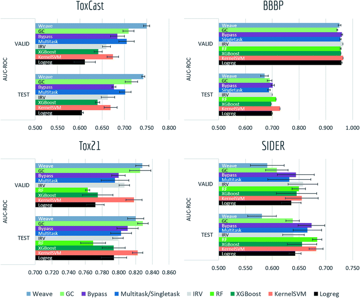
Tables S2, S3† and Fig. 7–9 report AUC-ROC or AUC-PRC results of 4 to 9 different models on biophysics datasets (PCBA, MUV, HIV, BACE) and physiology datasets (BBBP, Tox21, Toxcast, SIDER, ClinTox). Some models were too computationally expensive to be run on the larger datasets. All of these datasets contain only classification tasks.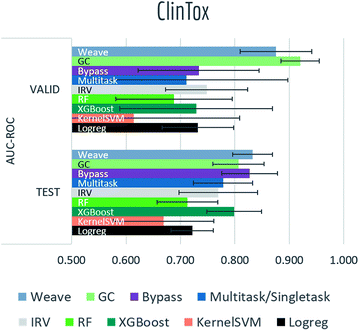 | ||
| Fig. 9 Benchmark performances for physiology tasks: ClinTox, 9 models are evaluated by AUC-ROC on random split. | ||
Most models have train scores (listed in Tables S2 and S3†) higher than validation/test scores, indicating that overfitting is a general issue. Singletask logistic regression exhibits the largest gaps between train scores and validation/test scores, while models incorporating multitask structure generally show less overfit, suggesting that multitask training has a regularizing effect. Most physiological and biophysical datasets in MoleculeNet have only a low volume of data for each task. Multitask algorithms combine different tasks, resulting in a larger pool of data for model training. In particular, multitask training can, to some extent, compensate for the limited data amount available for each individual task.
Graph convolutional models and weave models, each based on an adaptive method of featurization,22,23 show strong validation/test results on larger datasets, along with less overfit. Similar results are reported in previous graph-based algorithms,14,19,22,23,76 showing that learnable featurizations can provide a large boost compared with conventional featurizations.
For smaller singletask datasets (less than 3000 samples), differences between models are less clear. Kernel SVM and ensemble tree methods (gradient boosting and random forests) are more robust under data scarcity, while they generally need longer running time (see Table S1†). Worse performances of graph-based models are within expectation as complex models generally require more training data.
Bypass networks show higher train scores and equal or higher validation/test scores compared with vanilla multitask networks, suggesting that the bypass structure does add robustness. IRV models achieve performance broadly comparable with multitask networks. However, the quadratic nearest neighbor search makes the IRV models slower to train than the multitask networks (see Table S1†).
Three datasets (HIV, BACE, BBBP) in these two categories are evaluated under scaffold splitting. As compounds are divided by their molecular scaffolds, increasing differences between train, validation and test performances are observed. Scaffold splits provide a stronger test of a given model's generalizability compared with random splitting. Two datasets (PCBA, MUV) are evaluated by AUC-PRC, which is more practically useful under high class imbalance as discussed above. Graph convolutional model performs the best on PCBA (positive rate 1.40%), while results on MUV (positive rate 0.20%) are much less stable, which is most likely due to its extreme low amount of positive samples. Under such high imbalance, graph-based models are still not robust enough in controlling false positives.
Here we performed a more detailed experiment to illustrate how model performances change with increasing training samples. We trained multiple models on Tox21 with training sets of different size (10% to 90% of the whole dataset) Fig. 10 displayed mean out-of-sample performances (and standard deviations) of five independent runs. A clear increase on performance is observed for each model, and graph-based models (graph convolutional model and weave model) always stay on top of the lines. By drawing a horizontal line at around 0.80, we can see graph-based models achieve the similar level of accuracy with multitask networks by using only one-third of the training samples (30% versus 90%).
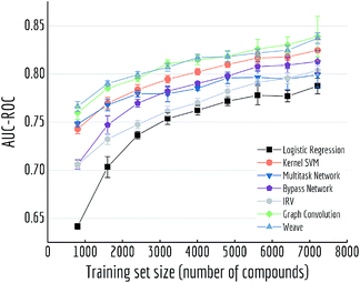 | ||
| Fig. 10 Out-of-sample performances with different training set sizes on Tox21. Each datapoint is the average of 5 independent runs, with standard deviations shown as error bars. | ||
4.2 Biophysics task – PDBbind
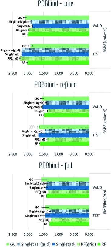
The PDBbind dataset maps distinct ligand–protein structures to their binding affinities. As discussed in the datasets section, we created grid featurizer to harness the joint ligand–protein structural information in PDBbind to build a model that predicts the experimental Ki of binding. We applied time splitting to all three subsets: core, refined, and full subsets of PDBbind (Core contains roughly 200 structures, refined 4000, and full 15![[thin space (1/6-em)]](https://www.rsc.org/images/entities/char_2009.gif) 000. The smaller datasets are cleaned more thoroughly than larger datasets.), with all results displayed in Table S4† and Fig. 11. Clearly as dataset size increased, we can see a significant boost on validation/test set performances. At the same time, for the two larger subsets: refined and full, switching from pure ligand-based ECFP to grid featurizer do increase the performances by a small margin in both Singletask networks and random forests. While for core subset, all models are showing relatively high errors and two featurizations do not show clear differences, which is within expectation as sample amount in core subset is too small to support a stable model performance. Note that models on the full set aren't significantly superior to models with less data; this effect may be due to the additional data being less clean.
000. The smaller datasets are cleaned more thoroughly than larger datasets.), with all results displayed in Table S4† and Fig. 11. Clearly as dataset size increased, we can see a significant boost on validation/test set performances. At the same time, for the two larger subsets: refined and full, switching from pure ligand-based ECFP to grid featurizer do increase the performances by a small margin in both Singletask networks and random forests. While for core subset, all models are showing relatively high errors and two featurizations do not show clear differences, which is within expectation as sample amount in core subset is too small to support a stable model performance. Note that models on the full set aren't significantly superior to models with less data; this effect may be due to the additional data being less clean.
Note that all models display heavy overfitting. Additional clean data may be required to create more accurate models for protein–ligand binding.
4.3 Physical chemistry tasks
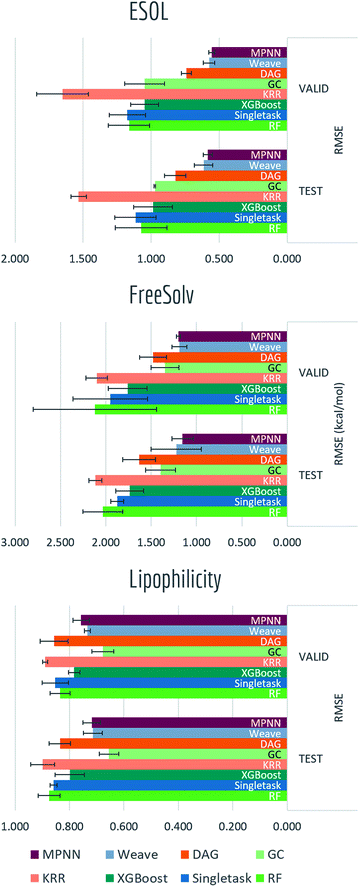
Solubility, solvation free energy and lipophilicity are basic physical chemistry properties important for understanding how molecules interact with solvents. Fig. 12 and Table S5† presented performances on predicting these properties.Graph-based methods: graph convolutional model, DAG, MPNN and weave model all exhibit significant boosts over vanilla singletask network, indicating the advantages of learnable featurizations. Differences between graph-based methods are rather minor and task-specific. The best-performing models in this category can already reach the accuracy level of ab initio predictions (±0.5 for ESOL, ±1.5 kcal mol−1 for FreeSolv).
We performed a more detailed comparison between data-driven methods and ab initio calculations on FreeSolv. Hydration free energy has been widely used as a test of computational chemistry methods. With free energy values ranging from −25.5 to 3.4 kcal mol−1 in the FreeSolv dataset, RMSE for calculated results reach up to 1.5 kcal mol−1.15 On the other hand, though machine learning methods typically need large amounts of training data to acquire predictive power, they can achieve higher accuracies given enough data. We investigate how the performance of machine learning methods on FreeSolv changes with the volume of training data. In particular, we want to know the amount of data required for machine learning to achieve accuracy similar to that of physically inspired algorithms.
For Fig. 13, we similarly generated a series of models with different training set volumes and calculated their out-of-sample RMSE. Each data point displayed is the average of 5 independent runs, with standard deviations displayed as error bars. Both graph convolutional model and weave model are capable of achieving better performances with enough training samples (30% and 50% of the data respectively). Given the size of FreeSolv dataset is only around 600 compounds, a weave model can reach state-of-the-art free energy calculation performances by training on merely 200 samples. On the other hand, comparing with singletask network's performance, weave model achieved the same level of accuracy with only one-third of the training samples.
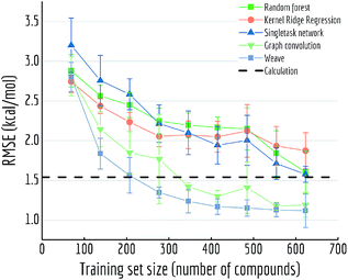 | ||
| Fig. 13 Out-of-sample performances with different training set sizes on FreeSolv. Each datapoint is the average of 5 independent runs, with standard deviations shown as error bars. | ||
4.4 Quantum mechanics tasks
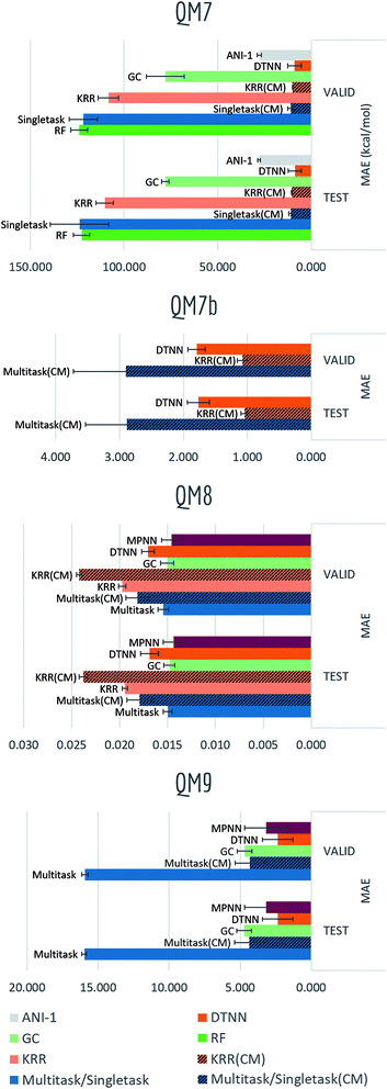
The QM datasets (QM7, QM7b, QM8, QM9) represent another distinct category of properties that are typically calculated through solving Schrödinger's equation (approximately using techniques such as DFT). As most conventional methods are slower than data-driven methods by orders of magnitude, we hope to learn effective approximators by training on existing datasets.Table S6† and Fig. 15 display the performances in mean absolute error of multiple methods. Tables S7–S9† show detailed performances for each task (due to difference in range of labels, mean performances of QM7b and QM9 are more skewed). Unsurprisingly, significant boosts on performances and less overfitting are observed for models incorporating distance information (multitask networks and KRR with Coulomb matrix featurization, DTNN, MPNN). In particular, KRR and multitask networks (CM) outperform their corresponding baseline models in QM7 and QM9 by a large margin, while DTNN and MPNN display less error comparing with graph convolutional models as well. At the same time, DTNN and MPNN gains better performances than multitask networks and KRR (CM) on most tasks. Table S7† shows that DTNN outperforms KRR (CM) on 12/14 tasks in QM7b (though the mean error shows the opposite result due to averaging errors on different magnitudes). In total, DTNN and MPNN covers the best-performing models on 28/39 of all tasks in this category, again reflecting the superiority of learnable featurization.
Another variable training size experiment is performed on QM7: predicting atomization energy. All mean absolute error performances are displayed in Fig. 14. Clearly incorporation of spatial position creates the huge gap between models, DTNN and multitask networks (CM) reach similar level of accuracy as reported in previous work on this dataset (there is still a gap between the MoleculeNet implementation and best reported numbers from previous work,18,19 which would likely be closed by training models longer). ANI-1 is also reported to achieve comparable performances on similar task in the previous work71 with a much larger dataset. Apparently its worse performance is restricted by training set size, as the MAE is keep decreasing with more training samples.
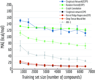 | ||
| Fig. 14 Out-of-sample performances with different training set sizes on QM7. Each datapoint is the average of 5 independent runs, with standard deviations shown as error bars. | ||
For QM series, proper choice of featurization appears critical. As mentioned previously, ECFP only consider graph substructures, while Coulomb matrix and graph featurizations used by DTNN and MPNN are explicitly calculated on charges and physical distances, which are exactly the required input for solving Schrödinger's equation.
5 Conclusions
This work introduces MoleculeNet, a benchmark for molecular machine learning. We gathered data for a wide range of molecular properties: 17 dataset collections including over 800 different tasks on 700![[thin space (1/6-em)]](https://www.rsc.org/images/entities/char_2009.gif) 000 compounds. Tasks are categorized into 4 levels as illustrated in Fig. 2: (i) quantum mechanical characters; (ii) physical chemistry properties; (iii) biophysical affinity and activity with bio-macromolecules; (iv) macroscopic physiological effects on human body.
000 compounds. Tasks are categorized into 4 levels as illustrated in Fig. 2: (i) quantum mechanical characters; (ii) physical chemistry properties; (iii) biophysical affinity and activity with bio-macromolecules; (iv) macroscopic physiological effects on human body.
MoleculeNet contributes a data-loading framework, featurization methods, data splitting methods, and learning models to the open source DeepChem package (Fig. 1). By adding interchangeable featurizations, splits and learning models into the DeepChem framework, we can apply these primitives to the wide range of datasets in MoleculeNet.
Broadly, our results show that graph-based models (graph convolutional models, weave models and DTNN) outperform other methods by comfortable margins on most datasets (11/17, best performances comparison in Table 3), revealing a clear advantage of learnable featurizations. However, this effect has some caveats: graph-based methods are not robust enough on complex tasks under data scarcity; on heavily imbalanced classification datasets, conventional methods such as kernel SVM outperform learnable featurizations with respect to recall of positives. Furthermore, for the PDBbind and quantum mechanics datasets, the use of appropriate featurizations which contains pertinent information is very significant. Comparing fully connected neural networks, random forests, and other comparatively simple algorithms, we claim that the PDBbind and QM7 results emphasize the necessity of using specialized features for different tasks. DTNN and MPNN which use distance information perform better on QM datasets than simple graph convolutions. While out of the scope of this paper, we note similarly that customized deep learning algorithms12 could in principle supplant the need for hand-derived, specialized features in such biophysical settings. On the FreeSolv dataset, comparison between conventional ab initio calculations and graph-based models for the prediction of solvation energies shows that data-driven methods can outperform physical algorithms with moderate amounts of data. These results suggest that data-driven physical chemistry will become increasingly important as methods mature. Results for biophysical and physiological datasets are currently weaker than for other datasets, suggesting that better featurizations or more data may be required for data-driven physiology to become broadly useful.
| Category | Dataset | Metric | Best performances – conventional methods | Best performances – graph-based methods |
|---|---|---|---|---|
| a As discussed in Section 4.4, DTNN outperforms KRR (CM) on 14/16 tasks in QM7b while the mean-MAE is skewed due to different magnitudes of labels. | ||||
| Quantum mechanics | QM7 | MAE | KRR (CM): 10.22 | DTNN: 8.75 |
| QM7b | MAE | KRR (CM): 1.05 | DTNN: 1.77 | |
| QM8 | MAE | Multitask: 0.0150 | MPNN: 0.0143 | |
| QM9 | MAE | Multitask (CM): 4.35 | DTNN: 2.35 | |
| Physical chemistry | ESOL | RMSE | XGBoost: 0.99 | MPNN: 0.58 |
| FreeSolv | RMSE | XGBoost: 1.74 | MPNN: 1.15 | |
| Lipophilicity | RMSE | XGBoost: 0.799 | GC: 0.655 | |
| Biophysics | PCBA | AUC-PRC | Logreg: 0.129 | GC: 0.136 |
| MUV | AUC-PRC | Multitask: 0.184 | Weave: 0.109 | |
| HIV | AUC-ROC | KernelSVM: 0.792 | GC: 0.763 | |
| BACE | AUC-ROC | RF: 0.867 | Weave: 0.806 | |
| PDBbind (full) | RMSE | RF(grid): 1.25 | GC: 1.44 | |
| Physiology | BBBP | AUC-ROC | KernelSVM: 0.729 | GC: 0.690 |
| Tox21 | AUC-ROC | KernelSVM: 0.822 | GC: 0.829 | |
| ToxCast | AUC-ROC | Multitask: 0.702 | Weave: 0.742 | |
| SIDER | AUC-ROC | RF: 0.684 | GC: 0.638 | |
| ClinTox | AUC-ROC | Bypass: 0.827 | Weave: 0.832 | |
By providing a uniform platform for comparison and evaluation, we hope MoleculeNet will facilitate the development of new methods for both chemistry and machine learning. In future work, we hope to extend MoleculeNet to cover a broader range of molecular properties than considered here. For example, 3D protein structure prediction, or DNA topological modeling would benefit from the presence of strong benchmarks to encourage algorithmic development. We hope that the open-source design of MoleculeNet will encourage researchers to contribute implementations of other novel algorithms to the benchmark suite. In time, we hope to see MoleculeNet grow into a comprehensive resource for the molecular machine learning community.
Conflicts of interest
There are no conflicts to declare.Acknowledgements
We would like to thank the Stanford Computing Resources for providing us with access to the Sherlock and Xstream GPU nodes. Thanks to Steven Kearnes and Patrick Riley for early discussions about the MoleculeNet concept. Thanks to Aarthi Ramsundar for help with diagram construction. Thanks to Zheng Xu for feedback on the MoleculeNet API. Thanks to Patrick Hop for contribution of the lipophilicity dataset to MoleculeNet. Thanks to Anthony Gitter and Johnny Israeli for suggesting the addition of AuPRC for imbalanced datasets. Thanks to Keri McKiernan for composing the tutorial of preparing datasets. The Pande Group is broadly supported by grants from the NIH (R01 GM062868 and U19 AI109662) as well as gift funds and contributions from Folding@home donors. We acknowledge the generous support of Dr Anders G. Frøseth and Mr Christian Sundt for our work on machine learning. B. R. was supported by the Fannie and John Hertz Foundation.References
- J. Gasteiger and J. Zupan, Angew. Chem., Int. Ed., 1993, 32, 503–527 CrossRef.
- J. Zupan and J. Gasteiger, Neural networks in chemistry and drug design, John Wiley & Sons, Inc., 1999 Search PubMed.
- A. Varnek and I. Baskin, J. Chem. Inf. Model., 2012, 52, 1413–1437 CrossRef CAS PubMed.
- J. B. Mitchell, Wiley Interdiscip. Rev.: Comput. Mol. Sci., 2014, 4, 468–481 CrossRef CAS PubMed.
- J. Devillers, Neural networks in QSAR and drug design, Academic Press, 1996 Search PubMed.
- G. Schneider and P. Wrede, Prog. Biophys. Mol. Biol., 1998, 70, 175–222 CrossRef CAS PubMed.
- Y. LeCun, Y. Bengio and G. Hinton, Nature, 2015, 521, 436–444 CrossRef CAS PubMed.
- J. Schmidhuber, Neural Network, 2015, 61, 85–117 CrossRef PubMed.
- J. Ma, R. P. Sheridan, A. Liaw, G. E. Dahl and V. Svetnik, J. Chem. Inf. Model., 2015, 55, 263–274 CrossRef CAS PubMed.
- B. Ramsundar, S. Kearnes, P. Riley, D. Webster, D. Konerding and V. Pande, 2015, arXiv preprint arXiv:1502.02072.
- T. Unterthiner, A. Mayr, G. Klambauer, M. Steijaert, J. Wenger, H. Ceulemans and S. Hochreiter, Deep Learning and Representation Learning Workshop (NIPS 2014), 2014 Search PubMed.
- I. Wallach, M. Dzamba and A. Heifets, 2015, arXiv preprint arXiv:1510.02855.
- J. S. Delaney, J. Chem. Inf. Model., 2004, 44, 1000–1005 CrossRef CAS PubMed.
- A. Lusci, G. Pollastri and P. Baldi, J. Chem. Inf. Model., 2013, 53, 1563–1575 CrossRef CAS PubMed.
- D. L. Mobley, K. L. Wymer, N. M. Lim and J. P. Guthrie, J. Comput.-Aided Mol. Des., 2014, 28, 135–150 CrossRef CAS PubMed.
- D. L. Mobley and J. P. Guthrie, J. Comput.-Aided Mol. Des., 2014, 28, 711–720 CrossRef CAS PubMed.
- M. Rupp, A. Tkatchenko, K.-R. Müller and O. A. V. Lilienfeld, Phys. Rev. Lett., 2012, 108, 058301 CrossRef PubMed.
- G. Montavon, M. Rupp, V. Gobre, A. Vazquez-Mayagoitia, K. Hansen, A. Tkatchenko, K.-R. Müller and O. A. V. Lilienfeld, New J. Phys., 2013, 15, 095003 CrossRef.
- K. T. Schütt, F. Arbabzadah, S. Chmiela, K. R. Müller and A. Tkatchenko, 2016, arXiv preprint arXiv:1609.08259.
- R. T. McGibbon, A. G. Taube, A. G. Donchev, K. Siva, F. Hernández, C. Hargus, K.-H. Law, J. L. Klepeis and D. E. Shaw, J. Chem. Phys., 2017, 147, 161725 CrossRef PubMed.
- D. Rogers and M. Hahn, J. Chem. Inf. Model., 2010, 50, 742–754 CrossRef CAS PubMed.
- D. Duvenaud, D. Maclaurin, J. Aguilera-Iparraguirre, R. Gómez-Bombarelli, T. Hirzel, A. Aspuru-Guzik and R. P. Adams, 2015, arXiv preprint arXiv:1509.09292.
- S. Kearnes, K. McCloskey, M. Berndl, V. Pande and P. Riley, 2016, arXiv preprint arXiv:1603.00856.
- G. A. Miller, Commun. ACM, 1995, 38, 39–41 CrossRef.
- J. Deng, W. Dong, R. Socher, L.-J. Li, K. Li and L. Fei-Fei, CVPR09, 2009 Search PubMed.
- O. Russakovsky, J. Deng, H. Su, J. Krause, S. Satheesh, S. Ma, Z. Huang, A. Karpathy, A. Khosla, M. Bernstein, A. C. Berg and L. Fei-Fei, Int. J. Comput. Vis., 2015, 115, 211–252 CrossRef.
- A. Krizhevsky, I. Sutskever and G. E. Hinton, NIPS Proceedings, 2012 Search PubMed.
- C. Szegedy, W. Liu, Y. Jia, P. Sermanet, S. Reed, D. Anguelov, D. Erhan, V. Vanhoucke and A. Rabinovich, 2014, arXiv preprint arXiv:1409.4842.
- K. He, X. Zhang, S. Ren and J. Sun, 2015, arXiv preprint arXiv:1512.03385.
- DeepChem: Deep-learning models for Drug Discovery and Quantum Chemistry, http://github.com/deepchem/deepchem, accessed 2017-09-27 Search PubMed.
- F. Pedregosa, G. Varoquaux, A. Gramfort, V. Michel, B. Thirion, O. Grisel, M. Blondel, P. Prettenhofer, R. Weiss and V. Dubourg, et al. , J. Mach. Learn. Res., 2011, 12, 2825–2830 Search PubMed.
- M. Abadi, A. Agarwal, P. Barham, E. Brevdo, Z. Chen, C. Citro, G. S. Corrado, A. Davis, J. Dean and M. Devin, et al., 2016, arXiv preprint arXiv:1603.04467.
- R. P. Sheridan, J. Chem. Inf. Model., 2013, 53, 783–790 CrossRef CAS PubMed.
- E. E. Bolton, Y. Wang, P. A. Thiessen and S. H. Bryant, Annu. Rep. Comput. Chem., 2008, 4, 217–241 CAS.
- T. Wang, J. Xiao, T. O. Suzek, J. Zhang, J. Wang, Z. Zhou, L. Han, K. Karapetyan, S. Dracheva, B. A. Shoemaker, E. Bolton, A. Gindulyte and S. H. Bryant, Nucleic Acids Res., 2012, 40, D400–D412 CrossRef PubMed.
- S. Gražulis, D. Chateigner, R. T. Downs, A. Yokochi, M. Quirós, L. Lutterotti, E. Manakova, J. Butkus, P. Moeck and A. Le Bail, J. Appl. Crystallogr., 2009, 42, 726–729 CrossRef PubMed.
- C. R. Groom, I. J. Bruno, M. P. Lightfoot and S. C. Ward, Acta Crystallogr., Sect. B: Struct. Sci., Cryst. Eng. Mater., 2016, 72, 171–179 CrossRef CAS PubMed.
- H. Berman, K. Henrick and H. Nakamura, Nat. Struct. Mol. Biol., 2003, 10, 980 CAS.
- Quantum Machine, http://quantum-machine.org/datasets/, accessed 2017-09-27 Search PubMed.
- D. Weininger, J. Chem. Inf. Comput. Sci., 1988, 28, 31–36 CrossRef CAS.
- L. C. Blum and J.-L. Reymond, J. Am. Chem. Soc., 2009, 131, 8732–8733 CrossRef CAS PubMed.
- R. Ramakrishnan, M. Hartmann, E. Tapavicza and O. A. V. Lilienfeld, J. Chem. Phys., 2015, 143, 084111 CrossRef PubMed.
- L. Ruddigkeit, R. V. Deursen, L. C. Blum and J.-L. Reymond, J. Chem. Inf. Model., 2012, 52, 2864–2875 CrossRef CAS PubMed.
- R. Ramakrishnan, P. O. Dral, M. Rupp and O. A. V. Lilienfeld, Sci. Data, 2014, 1, 140022 CAS.
- Experimental in vitro DMPK and physicochemical data on a set of publicly disclosed compounds.
- S. G. Rohrer and K. Baumann, J. Chem. Inf. Model., 2009, 49, 169–184 CrossRef CAS PubMed.
- AIDS Antiviral Screen Data, http://wiki.nci.nih.gov/display/NCIDTPdata/AIDS+Antiviral+Screen+Data, accessed 2017-09-27 Search PubMed.
- R. Wang, X. Fang, Y. Lu and S. Wang, J. Med. Chem., 2004, 47, 2977–2980 CrossRef CAS PubMed.
- R. Wang, X. Fang, Y. Lu, C.-Y. Yang and S. Wang, J. Med. Chem., 2005, 48, 4111–4119 CrossRef CAS PubMed.
- Z. Liu, Y. Li, L. Han, J. Li, J. Liu, Z. Zhao, W. Nie, Y. Liu and R. Wang, Bioinformatics, 2014, 31, 405–412 CrossRef PubMed.
- G. Subramanian, B. Ramsundar, V. Pande and R. A. Denny, J. Chem. Inf. Model., 2016, 56, 1936–1949 CrossRef CAS PubMed.
- I. F. Martins, A. L. Teixeira, L. Pinheiro and A. O. Falcao, J. Chem. Inf. Model., 2012, 52, 1686–1697 CrossRef CAS PubMed.
- Tox21 Challenge, http://tripod.nih.gov/tox21/challenge/, accessed 2017-09-27 Search PubMed.
- A. M. Richard, R. S. Judson, K. A. Houck, C. M. Grulke, P. Volarath, I. Thillainadarajah, C. Yang, J. Rathman, M. T. Martin, J. F. Wambaugh, T. B. Knudsen, J. Kancherla, K. Mansouri, G. Patlewicz, A. J. Williams, S. B. Little, K. M. Crofton and R. S. Thomas, Chem. Res. Toxicol., 2016, 29, 1225–1251 CrossRef CAS PubMed.
- M. Kuhn, I. Letunic, L. J. Jensen and P. Bork, Nucleic Acids Res., 2016, 44, D1075–D41079 CrossRef CAS PubMed.
- H. Altae-Tran, B. Ramsundar, A. S. Pappu and V. Pande, 2016, arXiv preprint arXiv:1611.03199.
- Medical Dictionary for Regulatory Activities, http://www.meddra.org/, accessed 2017-09-27 Search PubMed.
- K. M. Gayvert, N. S. Madhukar and O. Elemento, Cell Chem. Biol., 2016, 23, 1294–1301 CrossRef CAS PubMed.
- A. V. Artemov, E. Putin, Q. Vanhaelen, A. Aliper, I. V. Ozerov and A. Zhavoronkov, bioRxiv, Biochem., 2016, 095653 Search PubMed.
- P. A. Novick, O. F. Ortiz, J. Poelman, A. Y. Abdulhay and V. S. Pande, PLoS One, 2013, 8(11), e79568 CAS.
- Aggregate Analysis of ClincalTrials.gov (AACT) Database, http://www.ctti-clinicaltrials.org/aact-database, accessed 2017-09-27 Search PubMed.
- G. W. Bemis and M. A. Murcko, J. Med. Chem., 1996, 39, 2887–2893 CrossRef CAS PubMed.
- G. Landrum, RDKit: Open-Source Cheminformatics Software, http://www.rdkit.org/ Search PubMed.
- A. N. Jain and A. Nicholls, J. Comput.-Aided Mol. Des., 2008, 22, 133–139 CrossRef CAS PubMed.
- T. Hastie, R. Tibshirani and J. Friedman, The Elements of Statistical Learning: Data Mining, Inference, and Prediction, Springer, 2009 Search PubMed.
- J. Davis and M. Goadrich, Proceedings of the 23rd International Conference on Machine Learning, 2006 Search PubMed.
- R. Gómez-Bombarelli, D. Duvenaud, J. M. Hernández-Lobato, J. Aguilera-Iparraguirre, T. D. Hirzel, R. P. Adams and A. Aspuru-Guzik, 2016, arXiv preprint arXiv:1610.02415.
- J. D. Durrant and J. A. McCammon, J. Chem. Inf. Model., 2011, 51, 2897–2903 CrossRef CAS PubMed.
- C. Da and D. Kireev, J. Chem. Inf. Model., 2014, 54, 2555–2561 CrossRef CAS PubMed.
- J. Behler and M. Parrinello, Phys. Rev. Lett., 2007, 98, 146101 CrossRef PubMed.
- J. S. Smith, O. Isayev and A. E. Roitberg, 2016, arXiv preprint arXiv:1610.08935.
- L. Breiman, Mach. Learn., 2001, 45, 5–32 CrossRef.
- J. H. Friedman, Ann. Stat., 2001, 1189–1232 CrossRef.
- B. Ramsundar, B. Liu, Z. Wu, A. Verras, M. Tudor, R. P. Sheridan and V. Pande, J. Chem. Inf. Model., 2017, 57(8), 2068–2076 CrossRef CAS PubMed.
- S. J. Swamidass, C.-A. Azencott, T.-W. Lin, H. Gramajo, S.-C. Tsai and P. Baldi, J. Chem. Inf. Model., 2009, 49, 756–766 CrossRef CAS PubMed.
- J. Gilmer, S. S. Schoenholz, P. F. Riley, O. Vinyals and G. E. Dahl, 2017, arXiv preprint arXiv:1704.01212.
- J. Friedman, T. Hastie and R. Tibshirani, et al. , Ann. Stat., 2000, 28, 337–407 CrossRef.
- C. Cortes and V. Vapnik, Mach. Learn., 1995, 20, 273–297 Search PubMed.
- T. Chen and C. Guestrin, 2016, arXiv preprint arXiv:1603.02754.
- S. Kearnes, B. Goldman and V. Pande, 2016, arXiv preprint arXiv:1606.08793.
- I. I. Baskin, V. A. Palyulin and N. S. Zefirov, J. Chem. Inf. Comput. Sci., 1997, 37, 715–721 CrossRef CAS.
- D. B. Kireev, J. Chem. Inf. Comput. Sci., 1995, 35, 175–180 CrossRef CAS.
- O. Vinyals, S. Bengio and M. Kudlur, 2015, arXiv preprint arXiv:1511.06391.
Footnotes |
| † Electronic supplementary information (ESI) available. See DOI: 10.1039/c7sc02664a |
| ‡ Joint first authorship. |
| § Joint second authorship. |
| This journal is © The Royal Society of Chemistry 2018 |


