 Open Access Article
A quantitative structure–property study of reorganization energy for known p-type organic semiconductors†
Sule Atahan-Evrenk *
*
TOBB University of Economics and Technology, Faculty of Medicine, Sogutozu Cad No. 43, Sogutozu Ankara, Turkey. E-mail: satahanevrenk@etu.edu.tr; Fax: +90 312 292 44 32; Tel: +90 312 292 44 26
First published on 4th December 2018
Abstract
Intramolecular reorganization energy (RE), which quantifies the electron-phonon coupling strength, is an important charge transport parameter for the theoretical characterization of molecular organic semiconductors (OSCs). On a small scale, the accurate calculation of the RE is trivial; however, for large-scale screening, faster approaches are desirable. We investigate the structure–property relations and present a quantitative structure–property relationship study to facilitate the computation of RE from molecular structure. To this end, we generated a compound set of 171, which was derived from known p-type OSCs built from moieties such as acenes, thiophenes, and pentalenes. We show that simple structural descriptors such as the number of atoms, rings or rotatable bonds only weakly correlate with the RE. On the other hand, we show that regression models based on a more comprehensive representation of the molecules such as SMILES-based molecular signatures and geometry-based molecular transforms can predict the RE with a coefficient of determination of 0.7 and a mean absolute error of 40 meV in the library, in which the RE ranges from 76 to 480 meV. Our analysis indicates that a more extensive compound set for training is necessary for more predictive models.
1 Introduction
Organic semiconductors (OSCs) show remarkable (opto)electronic properties such as semiconductivity, electroluminescence and the photovoltaic effect.1 Owing to their potential for solution processability and compatibility with flexible substrates, they are ideal for low cost, flexible electronics.2,3 Moreover, the versatility of carbon allows for the discovery of new materials in a vast chemical compound space. Computational screening can facilitate the discovery of new OSCs by helping exploration of this chemical space at a low cost.4–7Understanding the relationship between molecular/crystal structure and charge transport is crucial to facilitate the synthesis of high-performance organic semiconductors (OSCs). However, a thorough de novo multi-scale study of charge carrier mobility in OSCs is a formidable task, especially for screening a large library of compounds. An alternative approach is to adopt a computational funnel, in which the resources are gradually focused on more promising molecules.6,8 For preliminary screening, quantitative structure–property relationship (QSPR) models that can predict material properties according to easily calculated descriptors based on the ground-state molecular structure are indispensable.
Here we focus on the reorganization energy (RE) as one such parameter for large-scale screening.8–10 Thermal hopping picture allows for a rapid evaluation of the RE at the molecular level. Unfortunately, it has only limited applicability (i.e. for materials with mobility values < 10−2 cm2 V−1 s−1).11 Despite this fact, the magnitude of the electronic coupling term relative to the magnitude of the RE is important for the determination of the charge transport regime.12,13 For single crystalline materials with strong electronic coupling, the decrease in the mobility as a function of increasing temperature has been shown to be a result of the localization of the charges due to the modulation of the electronic coupling terms, and not because of the RE. However, in these models a larger RE results in lower mobility values.12 For these reasons, as well as for its importance in charge carrier hopping, strategies adopting the RE as a parameter for preliminary large-scale screening are of value. We should note however that the charge transport performance of materials is ultimately determined by the crystal structure and the ensuing charge transport mechanisms.
Although gas-phase quantum chemical intramolecular RE calculations are trivial on a small scale, for large-scale screening faster calculation schemes are highly desirable. In this article, we present a new data set to explore structure–property relationships, as well as models for the prediction of the RE from molecular structure for p-type OSCs. If successful, such QSPR models might enable the use of the RE as a screening parameter in high-throughput approaches for choosing the best candidates for further higher level theoretical studies.
For data-driven materials research, reliable data sets for model training are crucial. However, most of the RE data for experimentally realized molecules is thinly spread in the literature. To date, there is no comprehensive data set which would enable systematic studies based on the RE. Moreover, the available quantum-chemical data were obtained at various levels of theory, therefore, it is hard to draw general trends from the structure–property relationship studies.
To the best of our knowledge, only two other attempts have been made to predict the RE using QSPR methodology. In one study, Misra et al. developed QSPR models for structure–mobility predictions for a library including only polyaromatic hydrocarbons (PAHs).10 Another smaller scale study14 used neural networks to predict the RE values for hole and electron hopping in carbon nanotubes. Both of the previous studies used compound libraries built only from fused benzene rings. Here we extend the structure–property study into a more diverse set of compounds which include many state-of-the-art molecular OSCs.
In this work, first we focus on the so-called interpretable QSPR models. These models relate the molecular and electronic structural features of the molecules with the intramolecular RE. The inspiration for these models usually stems from chemists’ observations that certain structural features lead to predictable behavior of the target property in a small set of molecules. How these trends are manifested in large and diverse compound sets is of interest. Second, we investigate the regression models, in particular the partial least squares (PLS) and the principle component regression (PCR), which are built using a more systematic representation of molecules, in which each atom, bond or connection type is included in the structural coding. We showed that despite the small size of the molecular library, these models show promising predictive potential.
1.1 Molecular library
Since the development of the first OFET with a polythiophene thin-film active layer,15 many heteroarene- and acene-based compounds have been synthesized as p-type OSCs for transistor applications.16 Over the years, compounds such as pentacene, oligothiophenes and their solution-processable forms have gained benchmark status. Thienoacenes, which are built from thiophene and acene units, have emerged as high-performance and high-stability OSCs.17 Therefore, we mostly restricted our library to experimentally known acenes, thiophenes, and thienoacenes. A few compounds with the antiaromatic pentalene moiety were also included for variety.18 In addition, we included building blocks, such as smaller acenes and thiophenes, and a few molecules from published computational screening studies. ESI Table 1† lists all 171 molecules included in this study in the order of increasing molecular weight, along with the electronic data and previously available RE values for comparison. This work presents the most comprehensive RE data to date for experimentally known p-type molecular OSCs.1.2 Reorganization energy
The RE is the total energy due to the deformation of the lattice and the molecular structure as the charge moves. In the weak electronic coupling limit, a site localized charge is assumed. Hence the largest contribution to the RE is due to the deformation at the molecular site. As such, the RE can be calculated from the total of the internal (intramolecular) and external (intermolecular) contributions: λ = λint + λext, where λint can be approximately calculated using the gas-phase geometry deformation upon charging.19 The external contribution λext is more challenging to calculate or measure and is highly dependent on the morphology.20–22 Although it is not possible to accurately describe the charge transport without the inclusion of λext,21 for preliminary screening purposes, λint can be sufficient.9,10By assuming a self-exchange hole transfer reaction, such as A + A+ → A+ + A, the reorganization energy can be calculated using λ = Ecn − Enn + Enc − Ecc. Here, Eji refers to the energy of the charge state j calculated at the optimized geometry i such that Ecn is the energy of the cation at the optimized neutral geometry. Those points over the potential energy surfaces are labeled in Fig. 1, which summarizes the computational scheme for the pentacene molecule. This scheme requires the optimization of the ground and cation states of the molecules in the gas phase, and two additional single points on the ground and cation potential energy surfaces.19 The most expensive step in this scheme is the calculation of the Hessian matrices of the optimized geometries necessary to ensure true minima.‡
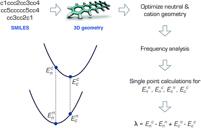 | ||
| Fig. 1 Calculation of the reorganization energy from the neutral and cation potential energy surfaces for pentacene. | ||
It is well known that density functional theory calculations are heavily influenced by the chosen density functional; for extended molecules, range-separated tuned functionals give better theoretical estimates for the RE. Nevertheless, the B3LYP functional employed here usually produces RE trends for p-type OSCs correctly,23 and hence has been widely used in charge transport studies of OSC materials.24 Although the experimental RE data for comparison is very limited, the values calculated from the B3LYP/6-31G(d,p) level of theory compare well with data from gas-phase photoelectron spectroscopy experiments, for example, with pentacene and perfluorpentacene.22
All the density functional theory calculations were performed using the Q-Chem software package25 at the level B3LYP26,27 with the Gaussian basis 6-31G(d,p)28–30 without any symmetry restrictions. The spin contamination in the cations was always less than 7%. All minima were ensured with the absence of negative vibrational frequencies through frequency analysis.
1.3 Molecular representations
The molecules were first written as SMILES strings31 and then represented as vectors either in the structural and electronic descriptor, the graph-based signature descriptor32 or the molecular transform descriptor33 spaces. The signatures were obtained from SMILES, whereas the molecular transforms required 3D geometries. In particular, we explored the molecular transforms obtained from MMFF94 (ref. 34) force field and density functional theory optimized geometries. In both cases, the ground state neutral molecular structures were used. For the molecules with a rotatable bond, we chose only the lowest energy conformer.The signature descriptors code the neighborhood of each atom in a molecule, starting with its immediate neighbors, and can be generated up to a desired height h. For example at h = 0, only the atom itself is included, and at height h = 1, its immediate neighbors are also included. Once all the atomic signatures of a molecular set have been identified for a particular height, each molecule can be represented as an array storing the frequency of each atomic signature in the molecule. Hence, for a molecular set of size N, a matrix with size N × Nsig is obtained, where Nsig is the total number of unique atomic signatures identified for the set. For simplicity, we refer to the total of number of signatures at a particular height n as σh0n.
The number of unique signatures necessary to describe the set increases rapidly. For example, in our molecular set, at σh00, there are only three signatures for sulphur, carbon, and hydrogen atom types. At σh01, σh02, σh03 and σh04, there are 16, 115, 590 and 1604 signatures, respectively. Previously, using signatures from up to height 3 (σh03) has been identified as sufficient to describe the RE.10 Therefore, we explored σh03 and σh04 in our analysis.
Naturally, overfitting is a problem when a matrix with a size of 171 × 605 or 171 × 1604 is to be solved. To combat overfitting, we explored dimensionality reduction algorithms such as the principle component analysis and partial least squares.
As the 3D structure descriptor, we used the molecular transform descriptors introduced previously by Soltzberg and Wilkins,33 and later adapted by Gasteiger and coworkers.35 The molecular transforms are approximate functions obtained from the 3D atomic coordinates of the molecules. They resemble a generalized scattering function from gas phase X-ray diffraction. By assuming that the molecule is a rigid body and the atoms are point scatterers (no form factors), the 3D coordinates of the molecule with N atoms can be converted into a molecular transform as follows:
 | (1) |
One advantage of the molecular transform is the fixed length, independent of the library size. The length of the molecular transform descriptors depends how precisely the parameter s is defined in the interval [1, 31]. We determined that 100 points is a good length for the regression models we studied.
For generating the molecular signatures, we used scripts developed by Faulon and coworkers.32 The molecular mechanics geometries were calculated with the ChemAxon molconvert utility. The structural descriptors such as the size, number of rings and type of atoms and bonds, as well as the polarizability and the van der Waals surface area were calculated with the cxcalc utility in the ChemAxon suite of programs. The data were managed and analyzed with modules such as the statsmodels36 and scikit learn37 available in the Python language.38
2 Results and discussion
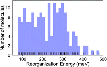
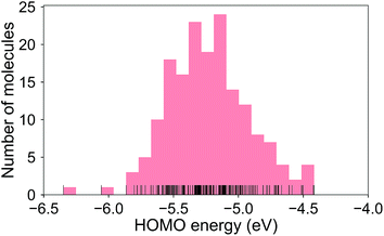
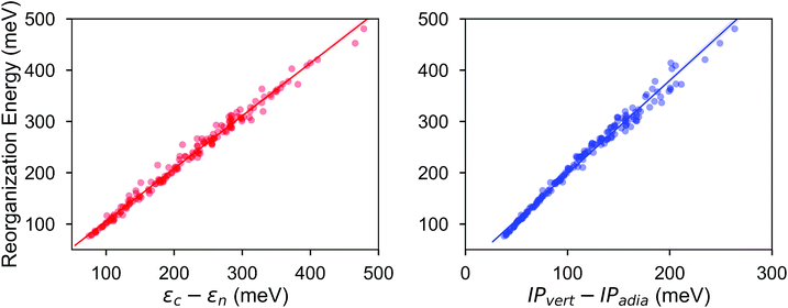
The calculated RE values range from 76 to 480 meV, positively skewed as expected from the high-performance OSCs (see histogram in Fig. 2). The ground-state highest occupied molecular orbital (HOMO) energies show a distribution typical of p-type OSCs with an average of −5.22 eV (see Fig. 3).The electronic data confirms the earlier HOMO eigenvalue difference descriptor derived from the neutral and cation HOMO energies as εhomoc − εhomon10 (Fig. 4a). The cation HOMO energy, εhomoc, refers to the energy at the HOMO energy for the optimized cation. Although this descriptor shows a very strong correlation with the RE, since we would like to limit the set of descriptors we can use to only the ground neutral state of the molecules, it is unsuitable for our QSPR methodology.
Taherpour et al.14 used both the adiabatic and vertical ionization potentials for the prediction of RE. Fig. 4b shows the RE as a regression of the difference between these ionization potentials. This difference is equal to the reorganization of the nuclei as the cation species form and relax into the optimum cation geometry,39,40 which can be formulated as Ecn − Ecc according to the potential energy surfaces shown in Fig. 1. It is, approximately, half of the RE as shown in Fig. 4 when similar relaxation energies are observed for the neutral and cation species. As shown in Fig. 4b, except for some of the high RE molecules which have an asymmetry in the relaxation of the charge donor and acceptor upon the vertical transitions and deviate slightly from the linear fit, the RE can be predicted from a linear relationship. Again, since we focus here only on the neutral state descriptors, this difference (IPvert − IPadia) is not useful for us as a descriptor.
First, we investigated the correlation of the electronic parameters with the RE. The total electronic energy, the HOMO and LUMO energy values and the vertical IP present a weak correlation with the RE. These descriptors, which are also correlated with each other, were not enough by themselves to establish a model for the prediction of the RE. Another electronic descriptor, which is potentially important for molecular electronic materials, is the polarizability.41 However, we show in Table 1 that the average molecular polarizability does not correlate with the RE. As explained above, we cannot use the adiabatic and vertical IP in the same model. Moreover, since the computation of the adiabatic IP requires the calculation of the optimum cation geometry, it does not satisfy our criterion that the descriptors should solely be calculated based on the neutral ground state of the compounds.
| Descriptor | Pearson’s r | p-Values |
|---|---|---|
| En | −0.20 | 0.0086 |
| εhomon | −0.20 | 0.0086 |
| εlumon | 0.16 | 0.03 |
| εhomoc | 0.076 | 0.32 |
| εlumoc | 0.046 | 0.55 |
| IPadia | 0.088 | 0.25 |
| IPvert | 0.19 | 0.014 |
| Average polarizability | −0.053 | 0.49 |
Owing to the importance of the RE, the structural factors affecting the magnitude of the RE have drawn considerable attention,24,42–46 for example, the length of the molecule46,47 or the presence of rotatable bonds.46,48,49 However, these observations are usually limited to a small series of compounds. For example, the RE decreases in a series of compounds from the shorter to longer oligomers46 or acenes.47,49 In a compound set with diverse molecular shapes, these simple structural features are not descriptive enough by themselves for a highly predictive QSPR model.10 Nevertheless, to observe the relationships in our data set, we investigated the correlation of the RE with structural descriptors such as the number of (fused) rings, the number of rotatable bonds, the van der Waals surface area and the sulphur atom count. Pearson’s r values for these are tabulated in Table 2. The largest correlation belongs to the fused ring count with −0.46; the rotatable bond and sulphur atom count follow with 0.44 and 0.34, respectively.
| Descriptor | Pearson’s r | p-Values |
|---|---|---|
| Fused ring count | −0.46 | 1.5 × 10⁻¹⁰ |
| Rotatable bond count | 0.44 | 2.1 × 10⁻⁹ |
| Sulphur atom count | 0.34 | 4.4 × 10⁻⁶ |
| van der Waals surface area | −0.052 | 0.50 |
| Ring count | −0.22 | 0.0046 |
We investigated the multiple linear regression (MLR) models built with the structural descriptors with p values smaller than 0.01, as well as some of the electronic descriptors. In ESI Table 2,† we show the correlation diagram of the electronic and structural descriptors with each other and the RE. Many of the variables show high correlation among themselves. Moreover, their correlation with the RE is weak. Only a few of these descriptors could be included in the model at a time with descriptive behaviour, a.k.a. with low p values. Therefore it was a challenge to obtain a predictive MLR model with this set of descriptor variables.
The best performing MLR model with the structural and electronic descriptors when all of the data points had been fitted to the model had an R2 of 0.49 (Radj2 = 0.48) (log![[thin space (1/6-em)]](https://www.rsc.org/images/entities/char_2009.gif) λ = 2.661 − 0.496εhomon (eV) − 0.055(ring count) + 0.077(sulphur atom count) + 0.141(rotatable bond count)). The test set performance was measured by randomly splitting the data into the test and training sets in the proportion 20/80, respectively. The average was obtained from 100 runs. The root mean squared error for the prediction of the RE values for the test set was quite large: 72 ± 10 meV and R2 = 0.31 ± 0.24. Due to this low performance, we investigated other descriptors which encode the molecular structures more systematically.
λ = 2.661 − 0.496εhomon (eV) − 0.055(ring count) + 0.077(sulphur atom count) + 0.141(rotatable bond count)). The test set performance was measured by randomly splitting the data into the test and training sets in the proportion 20/80, respectively. The average was obtained from 100 runs. The root mean squared error for the prediction of the RE values for the test set was quite large: 72 ± 10 meV and R2 = 0.31 ± 0.24. Due to this low performance, we investigated other descriptors which encode the molecular structures more systematically.
Unlike the descriptors used in the MLR model, the signatures encode the structural features of the molecules systematically including all atoms and the bond types, and in the case of the molecular transforms, information about the 3D geometry is also included to a certain extent. However, two major issues still emerge: (1) the large size of the descriptor space, especially in comparison to the library size (2) the correlation/collinearity in the descriptors. A transformation of the descriptor space onto a set of orthogonal principle components, such as in the case of the principle component analysis (PCA), might help combat both these issues at once. By careful analysis of the train and validation set errors, it is possible to determine the necessary number of principle components for a model that does not overfit. We report the results from this type of regression as principle component regression, PCR.
The distribution of the molecules labeled according to the RE values in the first three principle components for σh03 is shown in Fig. 5 (the ratio of the variance explained by each principle component is shown in ESI Fig. 2†). The color distribution indicates that the components can help organize data according to the magnitude of the RE. We observed a similar distribution for a deeper signature set, σh04. However, the principle components of the molecular transforms did not organize the molecules in a meaningful way related to the RE values. Therefore, the PCR models based on the molecular transforms are not included.
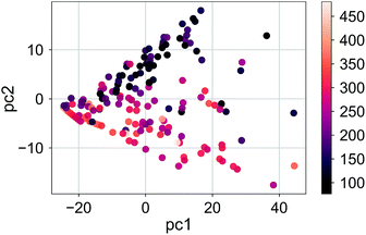 | ||
| Fig. 5 The RE values (meV) of the compound set scattered in the first two principle components for the signatures up to the height 3, σh03. | ||
The principle components were chosen to explain the variance in the descriptor space only, and are thus not very effective in the prediction. As an alternative regression approach, we investigated partial least squares (PLS) algorithms. The advantage of the PLS method is that a set of vectors which capture most of the variance in the descriptors is found while the correlation between the descriptor space and target RE values is also taken into consideration. For the PLS implementation we used the default version in python scikit learn (NIPALS algoritm).
The results from both the regression methods can be found in Table 3. The data for the test performances were obtained by 5-fold cross validation (20% test). The computations were repeated 100 times through random shuffling to gather enough statistics. In parenthesis are the number of principle component vectors (PCR) or latent variables (PLS) chosen with cross-validation. These numbers correspond to the number of vectors included in the models for which the test set performance is reported.
| Descriptor type | Modela | Rtrain2 | Rtest2 | Rtestrank | RMSEb | MAEb |
|---|---|---|---|---|---|---|
| a Numbers in parenthesis represent the size of the descriptor space.b The root mean squared error (RMSE) and mean absolute error (MAE) in meV. The statistics were obtained from 100 runs, where the data was shuffled randomly each time. | ||||||
| Signatures | σ03 | |||||
| PLS (5) | 0.96 ± 0.00 | 0.69 ± 0.09 | 0.81 ± 0.06 | 55 ± 8 | 41 ± 6 | |
| PCR (8) | 0.62 ± 0.02 | 0.57 ± 0.09 | 0.78 ± 0.06 | 57 ± 8 | 43 ± 6 | |
| σ04 | ||||||
| PLS (8) | 0.99 ± 0.00 | 0.70 ± 0.09 | 0.82 ± 0.06 | 54 ± 8 | 39 ± 7 | |
| PCR (16) | 0.67 ± 0.02 | 0.58 ± 0.10 | 0.79 ± 0.06 | 56 ± 7 | 42 ± 6 | |
| Transforms | DFT | |||||
| PLS (7) | 0.85 ± 0.01 | 0.66 ± 0.12 | 0.81 ± 0.06 | 60 ± 15 | 43 ± 7 | |
| MM | ||||||
| PLS (5) | 0.79 ± 0.01 | 0.62 ± 0.11 | 0.77 ± 0.07 | 60 ± 9 | 44 ± 6 | |
The best test performance belongs to the PLS models with the signature descriptors. The performance of the two signature levels, σh03 and σh04, was close. These results improved upon our earlier MLR models and the prediction statistics were comparable to those of previous models.10 However, the discrepancy between the test and train performances especially in the PLS models is large which shows that one avenue for the improvement of the models could be the expansion of the data set. On the other hand, the PCR models showed less predictive accuracy than the PLS models, as expected. In those models, the train and test performances were similar. The molecular transforms based on the DFT optimized geometries were significantly better both in the test and train sets than the MMFF94 predicted geometries. The Spearman rank correlation coefficients show that the ranking based on the DFT geometry derived molecular transform is as accurate as the PLS models for the σh03, although the average Rtest2 is smaller than that for the PLS model.
Finally, we show the pair plot for the best performing model in Fig. 6. Some of the outliers (errors larger than 100 meV) are marked with their molecule number from ESI Table 1.† These outliers could be explained to a certain extent in terms of molecular similarity. For example, molecule 140 stands out with a large overestimation. This is not surprising since this molecule has a sulfur atom with a bonding pattern which does not exist in any of the other compounds. Therefore, the training of the model does not cover the pattern of this molecule. The same could be said for molecule 26 with the unusual annulene pattern. There is again a large error for molecule number 1, the thiophene ring, which is the only monocycle in the library. The predictions for the molecules with two rings, thienothiophene (3) and dithienyl (5), are also poor. On the other hand the prediction error for diphenyl or naphthalene is not large, although there are not many molecules with two rings in the library.
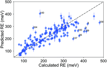 | ||
| Fig. 6 Comparison of the average predicted and calculated values of RE with the PLS model for the σh04 signature set. The data was collected from a 5-fold CV with 100 runs. The error bars are the standard deviations. The molecules with errors larger than 100 meV are marked with their number from ESI Table 1.† | ||
Due to the difficulty of the analysis of each molecule one-by-one and conflicting observations such as those mentioned above, we systematically investigated the hypothesis that a molecular (dis)similarity is correlated with the errors as follows. First, we calculated a similarity matrix for all of the molecules based on the Tanimoto metric. Then we counted the number of similar molecules for each molecule with a Tanimoto index cutoff of 0.85. We show a regression of the absolute error over this count in Fig. 7. Although it is small, we observe a negative slope for the fit, indicating that for most molecules with a high count of similar molecules, we observe smaller errors.
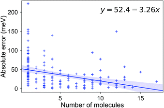 | ||
| Fig. 7 The absolute error (meV) in the RE for a molecule, as a function of the number of molecules with a Tanimoto coefficient larger than 0.85. | ||
3 Conclusions
We presented a new library of computed reorganization energy values for experimentally known OSCs and investigated several regression models for the prediction of the RE from molecular structure. Our best model was the PLS regression based on molecular signature descriptors. We observed that the size and diversity of the training set is crucial for the establishment of predictive and generalizable models. The discrepancy between the test and train performances in the PLS models indicates that to reduce the model bias, a larger molecular library will be necessary. We estimate that the library size needs to be at least in the order of thousands of compounds. The construction of a library of this size restricted to known OSC molecules could be challenging, and hence a combinatorially generated training set with potential OSC molecules might be necessary.Nevertheless, for the present molecular library, the prediction accuracy of the models (Rtest2 up to 0.7) with descriptors based on the ground-state properties of the compounds is remarkable as the RE is a parameter that measures the difficulty for a molecule to undergo hole exchange. Therefore, any higher accuracy prediction should include the effects of the adjustment of the nuclei on the charging process. Work is under way in our laboratory in the direction of the extension of the library and in investigation of higher level molecular descriptors for the representation of the molecules. This work also illustrates the potential of the present approach for the prediction of the RE for electron and exciton transport materials.
Conflicts of interest
There are no conflicts to declare.Acknowledgements
S. A. E. acknowledges financial support from TUBITAK BIDEB 2232 (Grant No. 114C153) and software support from ChemAxon Ltd.Notes and references
- A. Kohler and H. Bassler, Electronic Processes in Organic Semiconductors: An Introduction, 1st edn, Wiley-VCH Verlag GmbH & Co., Weinheim, Germany, 2015 Search PubMed.
- H. Klauk, Organic Electronics: Materials, Manufacturing, and Applications, 1st edn, Wiley-VCH Verlag GmbH & Co., Weinheim, Germany, 2006 Search PubMed.
- H. Klauk, Organic Electronics II: More Materials and Applications, 1st edn, Wiley-VCH Verlag GmbH & Co., Weinheim, Germany, 2012 Search PubMed.
- B. Baumeier, F. May, C. Lennartz and D. Andrienko, J. Mater. Chem., 2012, 22, 10971–10976 RSC.
- I. Y. Kanal, S. G. Owens, J. S. Bechtel and G. R. Hutchison, J. Phys. Chem. Lett., 2013, 4, 1613–1623 CrossRef CAS PubMed.
- E. O. Pyzer-Knapp, C. Suh, R. Gomez-Bombarelli, J. Aguilera-Iparraguirre and A. Aspuru-Guzik, Annu. Rev. Mater. Res., 2015, 45, 195–216 CrossRef CAS.
- L. H. Nguyen and T. N. Truong, ACS Omega, 2018, 3, 8913–8922 CrossRef CAS.
- C. Schober, K. Reuter and H. Oberhofer, J. Phys. Chem. Lett., 2016, 7, 3973–3977 CrossRef CAS PubMed.
- A. N. Sokolov, S. Atahan-Evrenk, R. Mondal, H. B. Akkerman, R. S. Sánchez-Carrera, S. Granados-Focil, J. Schrier, S. C. B. Mannsfeld, A. P. Zoombelt, Z. Bao and A. Aspuru-Guzik, Nat. Commun., 2011, 2, 437–438 CrossRef PubMed.
- M. Misra, D. Andrienko, B. Baumeier, J.-L. Faulon and O. A. von Lilienfeld, J. Chem. Theory Comput., 2011, 7, 2549–2555 CrossRef CAS PubMed.
- H. Oberhofer, K. Reuter and J. Blumberger, Chem. Rev., 2017, 117, 10319–10357 CrossRef CAS PubMed.
- A. Troisi, Chem. Soc. Rev., 2011, 40, 2347–2358 RSC.
- S. Giannini, A. Carof and J. Blumberger, J. Phys. Chem. Lett., 2018, 9, 3116–3123 CrossRef CAS PubMed.
- A. A. Taherpour, A. Aghagolnezhad-Gerdroudbari and S. Rafiei, Int. J. Electrochem. Sci., 2012, 7, 2468–2486 CAS.
- A. Tsumura, H. Koezuka and T. Ando, Appl. Phys. Lett., 1986, 49, 1210–1212 CrossRef CAS.
- C. Wang, H. Dong, W. Hu, Y. Liu and D. Zhu, Chem. Rev., 2012, 112, 2208–2267 CrossRef CAS PubMed.
- K. Takimiya, S. Shinamura, I. Osaka and E. Miyazaki, Adv. Mater., 2011, 23, 4347–4370 CrossRef CAS PubMed.
- S. Kato, S. Kuwako, N. Takahashi, T. Kijima and Y. Nakamura, J. Org. Chem., 2016, 81, 7700–7710 CrossRef CAS PubMed.
- V. Coropceanu, J. Cornil, D. A. da Silva Filho, Y. Olivier, R. Silbey and J.-L. Brédas, Chem. Rev., 2007, 107, 926–952 CrossRef CAS PubMed.
- J. E. Norton and J.-L. Bredas, J. Am. Chem. Soc., 2008, 130, 12377–12384 CrossRef CAS PubMed.
- D. P. McMahon and A. Troisi, J. Phys. Chem. Lett., 2010, 1, 941–946 CrossRef CAS.
- S. Kera, S. Hosoumi, K. Sato, H. Fukagawa, S.-i. Nagamatsu, Y. Sakamoto, T. Suzuki, H. Huang, W. Chen, A. T. S. Wee, V. Coropceanu and N. Ueno, J. Phys. Chem. C, 2013, 117, 22428–22437 CrossRef CAS.
- C. Brückner and B. Engels, J. Comput. Chem., 2016, 37, 1335–1344 CrossRef PubMed.
- H. Geng, Y. Niu, Q. Peng, Z. Shuai, V. Coropceanu and J. L. Brédas, J. Chem. Phys., 2011, 135, 104703 CrossRef PubMed.
- Y. Shao, Z. Gan, E. Epifanovsky, A. T. Gilbert, M. Wormit, J. Kussmann, A. W. Lange, A. Behn, J. Deng, X. Feng, D. Ghosh, M. Goldey, P. R. Horn, L. D. Jacobson, I. Kaliman, R. Z. Khaliullin, T. Kuś, A. Landau, J. Liu, E. I. Proynov, Y. M. Rhee, R. M. Richard, M. A. Rohrdanz, R. P. Steele, E. J. Sundstrom, H. L. Woodcock III, P. M. Zimmerman, D. Zuev, B. Albrecht, E. Alguire, B. Austin, G. J. O. Beran, Y. A. Bernard, E. Berquist, K. Brandhorst, K. B. Bravaya, S. T. Brown, D. Casanova, C.-M. Chang, Y. Chen, S. H. Chien, K. D. Closser, D. L. Crittenden, M. Diedenhofen, R. A. DiSastio Jr, H. Do, A. D. Dutoi, R. G. Edgar, S. Fatehi, L. Fusti-Molnar, A. Ghysels, A. Golubeva-Zadorozhnaya, J. Gomes, M. W. Hanson-Heine, P. H. Harbach, A. W. Hauser, E. G. Hohenstein, Z. C. Holden, T.-C. Jagau, H. Ji, B. Kaduk, K. Khistyaev, J. Kim, J. Kim, R. A. King, P. Klunzinger, D. Kosenkov, T. Kowalczyk, C. M. Krauter, K. U. Lao, A. D. Laurent, K. V. Lawler, S. V. Levchenko, C. Y. Lin, F. Liu, E. Livshits, R. C. Lochan, A. Luenser, P. Manohar, S. F. Manzer, S.-P. Mao, N. Mardirossian, A. V. Marenich, S. A. Maurer, N. J. Mayhall, E. Neuscamman, C. M. Oana, R. Olivares-Amaya, D. P. O’Neill, J. A. Parkhill, T. M. Perrine, R. Peverati, A. Prociuk, D. R. Rehn, E. Rosta, N. J. Russ, S. M. Sharada, S. Sharma, D. W. Small, A. Sodt, T. Stein, D. Stück, Y.-C. Su, A. J. Thom, T. Tsuchimochi, V. Vanovschi, L. Vogt, O. Vydrov, T. Wang, M. A. Watson, J. Wenzel, A. White, C. F. Williams, J. Yang, S. Yeganeh, S. R. Yost, Z.-Q. You, I. Y. Zhang, X. Zhang, Y. Zhao, B. R. Brooks, G. K. Chan, D. M. Chipman, C. J. Cramer, W. A. Goddard III, M. S. Gordon, W. J. Hehre, A. Klamt, H. F. Schaefer III, M. W. Schmidt, C. D. Sherrill, D. G. Truhlar, A. Warshel, X. Xu, A. Aspuru-Guzik, R. Baer, A. T. Bell, N. A. Besley, J.-D. Chai, A. Dreuw, B. D. Dunietz, T. R. Furlani, S. R. Gwaltney, C.-P. Hsu, Y. Jung, J. Kong, D. S. Lambrecht, W. Liang, C. Ochsenfeld, V. A. Rassolov, L. V. Slipchenko, J. E. Subotnik, T. V. Voorhis, J. M. Herbert, A. I. Krylov, P. M. Gill and M. Head-Gordon, Mol. Phys., 2015, 113, 184–215 CrossRef CAS.
- A. D. Becke, J. Chem. Phys., 1993, 98, 5648–5652 CrossRef CAS.
- C. Lee, W. Yang and R. G. Parr, Phys. Rev. B, 1988, 37, 785–789 CrossRef CAS.
- W. J. Hehre, R. Ditchfield and J. A. Pople, J. Chem. Phys., 1972, 56, 2257–2261 CrossRef CAS.
- M. M. Francl, W. J. Pietro, W. J. Hehre, J. S. Binkley, M. S. Gordon, D. J. Defrees and J. A. Pople, J. Chem. Phys., 1982, 77, 3654–3665 CrossRef CAS.
- P. C. Hariharan and J. A. Pople, Theor. Chim. Acta, 1973, 28, 213–222 CrossRef CAS.
- D. Weininger, J. Chem. Inf. Comput. Sci., 1988, 28, 31–36 CrossRef CAS.
- J.-L. Faulon, D. P. Visco and R. S. Pophale, J. Chem. Inf. Comput. Sci., 2003, 43, 707–720 CrossRef CAS PubMed.
- L. J. Soltzberg and C. L. Wilkins, J. Am. Chem. Soc., 1977, 2, 439–443 CrossRef.
- T. A. Halgren, J. Comput. Chem., 1996, 17, 553–586 CrossRef CAS.
- J. Schuur and J. Gasteiger, Anal. Chem., 1997, 69, 2398–2405 CrossRef CAS PubMed.
- J. Seabold and J. Perktold, Proceedings of the 9th Python in Science Conference, 2010 Search PubMed.
- F. Pedregosa, G. Varoquaux, A. Gramfort, V. Michel, B. Thirion, O. Grisel, M. Blondel, P. Prettenhofer, R. Weiss, V. Dubourg, J. Vanderplas, A. Passos, D. Cournapeau, M. Brucher, M. Perrot and E. Duchesnay, J. Mach. Learn. Res., 2011, 12, 2825–2830 Search PubMed.
- Python, 2016, https://www.python.org/.
- M. Meot-Ner, S. F. Nelsen, M. F. Willi and T. B. Frigo, J. Am. Chem. Soc., 1984, 106, 7384–7389 CrossRef CAS.
- S. F. Nelsen, S. C. Blackstock and Y. Kim, J. Am. Chem. Soc., 1987, 109, 677–682 CrossRef CAS.
- E. A. Silinsh, Organic Molecular Crystals: Their Electronic States, 1st edn, Springer-Verlag, Berlin Heidelberg, 1980 Search PubMed.
- R. Zhu, Y.-A. Duan, Y. Geng, C.-Y. Wei, X.-Y. Chen and Y. Liao, Comput. Theor. Chem., 2016, 1078, 16–22 CrossRef CAS.
- M. Mamada and Y. Yamashita, in S-Containing Polycyclic Heteroarenes: Thiophene-Fused and Thiadiazole-Fused Arenes as Organic Semiconductors, Wiley-VCH Verlag GmbH & Co. KGaA, 2015, pp. 277–308 Search PubMed.
- H.-Y. Chen and I. Chao, ChemPhysChem, 2006, 7, 2003–2007 CrossRef CAS PubMed.
- V. Coropceanu, O. Kwon, B. Wex, B. R. Kaafarani, N. E. Gruhn, J. C. Durivage, D. C. Neckers and J.-L. Brédas, Chem.–Eur. J., 2006, 12, 2073–2080 CrossRef CAS PubMed.
- G. R. Hutchison, M. A. Ratner and T. J. Marks, J. Am. Chem. Soc., 2005, 127, 2339–2350 CrossRef CAS PubMed.
- W.-Q. Deng and W. A. Goddard, J. Phys. Chem. B, 2004, 108, 8614–8621 CrossRef CAS.
- D. A. da Silva Filho, V. Coropceanu, D. Fichou, N. E. Gruhn, T. G. Bill, J. Gierschner, J. Cornil and J.-L. Brédas, Philos. Trans. R. Soc., A, 2007, 365, 1435–1452 CrossRef CAS PubMed.
- S. Atahan-Evrenk and A. Aspuru-Guzik, Top. Curr. Chem., 2014, 345, 95–138 CrossRef CAS PubMed.
Footnotes |
| † Electronic supplementary information (ESI) available: The electronic data for the molecular library, the structural and electronic descriptors correlation matrix, explained variance by principle components and pentacene molecular transform plot. See DOI: 10.1039/c8ra07866a |
| ‡ For example, for molecule number 109 in ESI Table 1† (232 electrons), of the 45 hours of computing time at the level B3LYP/6-31G(d,p), approximately 8 hours were dedicated to the Hessian calculation for the neutral ground state and 31 hours were dedicated to the Hessian calculation of the cation (calculated with Q-Chem 4.0 on four Intel Xeon(R) CPU E3-1246 v3 3.50 GHz processors). |
| This journal is © The Royal Society of Chemistry 2018 |

