
 Open Access Article
 This Open Access Article is licensed under a Creative Commons Attribution-Non Commercial 3.0 Unported Licence
Coherency image analysis to quantify collagen architecture: implications in scar assessment†
T. D. Clemons *a,
M. Bradshawa,
P. Toshniwala,
N. Chaudharia,
A. W. Stevensonb,
J. Lynchbc,
M. W. Fearb,
F. M. Woodb and
K. Swaminathan Iyer*a
*a,
M. Bradshawa,
P. Toshniwala,
N. Chaudharia,
A. W. Stevensonb,
J. Lynchbc,
M. W. Fearb,
F. M. Woodb and
K. Swaminathan Iyer*a
aSchool of Molecular Sciences M313, The University of Western Australia, 35 Stirling Hwy, Crawley, WA 6009, Australia. E-mail: tristan.clemons@uwa.edu.au; swaminatha.iyer@uwa.edu.au
bFiona Wood Foundation and Burn Injury Research Unit, The University of Western Australia, M318, 35 Stirling Hwy, Crawley, WA 6009, Australia
cRoyal College of Surgeon's of Ireland, 123 St Stephen's Green, Dublin, Ireland
First published on 6th March 2018
Abstract
An important histological difference between normal, uninjured dermis and scar tissue such as that found in keloid scars is the pattern (morphological architecture) in which the collagen is deposited and arranged. In the uninjured dermis, collagen bundle architecture appears randomly organized (or in a basket weave formation), whereas in pathological conditions such as keloid scar tissue, collagen bundles are often found in whorls or in a hypotrophic scar collagen is more densely packed in a parallel configuration. In the case of skin, a scar disables the dermis, leaving it weaker, stiff and with a loss of optimal functionality. The absence of objective and quantifiable assessments of collagen orientation is a major bottleneck in monitoring progression of scar therapeutics. In this article, a novel quantitative approach for analyzing collagen orientation is reported. The methodology is demonstrated using collagen produced by cells in a model scar environment and examines collagen remodeling post-TGFβ stimulation in vitro. The method is shown to be reliable and effective in identifying significant coherency differences in the collagen deposited by human keloid scar cells. The technique is also compared for analysing collagen architecture in rat sections of normal, scarred skin and tendon tissue. Results demonstrate that the proposed computational method provides a fast and robust way of analyzing collagen orientation in a manner surpassing existing methods. This study establishes this methodology as a preliminary means of monitoring in vitro and in tissue treatment modalities which are expected to alter collagen morphology.
Introduction
Accurate assessment of scars is important in the clinical evaluation and follow-up of patient treatment. It is essential to compare different treatment modalities clinically and monitor patient progression.1,2 Not only would an objective method of scar evaluation be useful for the well-being of the patient, but for legal reasons; providing an objective qualifier for reimbursement and proof of disability. To date, there is no consensus with regards to the optimal tool for scar assessment.3,4 An optimal assessment would perfectly model the important characteristics of the scar as well as accurately document the scar's evolution in response to treatment.5 Currently, scar scales such as the Vancouver Scar Scale (VSS), generally assess properties of the scar such as colour, pliability and thickness.6 They may also document physical limitations such as pain, limited mobility and itching whilst some scales will also include psychological impacts.5,7,8 These are all qualitative measures and have been shown to be highly observer dependent.9,10 The main reason why these types of scales are so dependent on the observer is the subjective nature of the description for the scar. For example in the VSS pliability is scored on a scale of zero to five, with the identifiers being: normal, supple, yielding, firm, banding and contracture. The difference between ‘supple’ and ‘yielding’ is clearly observer dependant and this inter-rater variability across all the measures for the scar can lead to large variability amongst scores. This inter-rater variability can be measured to assess the reproducibility of different scar assessment methods, with many studies reporting considerable variations between assessors and even between assessments using the same assessor.1,11,12 With this variability, the severity of a scar cannot be accurately reported and in turn the optimum treatment for that scar is difficult to determine and administer. However, scar scales as a tool are inexpensive and require little training or equipment. They do not necessarily increase workload and can be conducted quickly. This is in contrast to objective scar tools which comparatively require expensive pieces of instrumentation, require highly specialised training and can be time consuming for the assessor.7 To assess scars accurately, and to monitor a new treatment plan in a laboratory or clinical environment, a precise, reproducible, objective scar assessment tool is required.There are a number of factors that are different between scar and normal uninjured dermis. With respect to collagen this includes collagen density, thickness of collagen fibres and orientation. Other differences, dependent in part on extent of the burn injury sustained but can include lack of adnexal structures and changes to elastin and other matrix proteins. Since collagen is by far the most dominant protein present in dermal matrix of both scar and normal skin and hence the majority of measurement techniques have been based on analysing different aspects of the collagen architecture. To date, accurate and reproducible methods for quantitatively assessing collagen architecture in scars are lacking. Histological stains, such as Masson's trichrome and picrosirius red have been used to identify collagen abundance in tissue sections which can then be used for qualitative assessments of collagen integrity between samples.13,14 Confocal microscopy followed by fractal and lacunarity analysis has been proposed as a superior tool for the discrimination of scar collagen versus normal tissue.15 The results from the analysis correlated well with transmission electron microscopy images of the collagen ultrastructure and this type of analysis has previously been reported to be accurate and reproducible when applied to neurons, alveoli and capillary beds.16–18 Recently, sophisticated methods exploiting frequency domain transformation and power spectral analysis have been employed to try and solve the problem of collagen morphology quantitation.19,20 Power spectral analysis estimates the power variation of an image over different frequency ranges. It describes in energy terms how closely two points are related in an image as a function of distance and orientation.21 Fourier transforms, in particular the Fast Fourier Transform (FFT), has been used to estimate the power spectrum of images, and this approach has been directed at collagen fibre orientation and collagen bundle thickness and/or spacing.22–24
Research is continuing into new methods for quantitating collagen in scar tissue. Quinn, et al. recently developed an image analysis technique for the quantification of collagen alignment at a pixel-by-pixel level.25 This study was able to quantitatively assess significant differences between the collagen alignment in scars compared to normal tissue from rats at 2 and 6 months following the injury.25 However, there continues to be a need to develop more reliable, accurate and reproducible objective measures for collagen morphology. Here, coherency analysis is demonstrated to be a reliable method of quantifying collagen architecture and a highly effective alternative to existing objective scar assessment measures including Fourier analysis and collagen orientation index (COI) as a means of quantifying collagen alignment. A summary of current methodologies from within the literature and a comparison of their key findings with that of the coherency protocol outlined within this paper is provided in the ESI (See ESI Table S1†).
Materials and methods
In this section we describe the details of the experimental protocol followed for the generation of typical data for image analysis.Cell culture
The protocol used for in vitro analysis was adapted from the ‘scar in a jar’ protocol developed by Chen et al.26 Primary dermal scar fibroblasts at passage 5 were trypsinised and seeded into Nunc™ Lab-Tek® chamber slides with Permanox® plastic to achieve 50![[thin space (1/6-em)]](https://www.rsc.org/images/entities/char_2009.gif) 000 cells per well in normal growth media Dulbecco's Modified Eagle Medium GlutaMax (DMEM, Life Technologies) supplemented with 10% foetal bovine serum (FBS, Interpath) and 1% v/v penicillin/streptomycin (Life Technologies). After 16 hours of culture at 37 °C and 5% CO2 (g), the media was changed to a crowding media. The composition of the crowding media was as follows: for 10 mL; L-ascorbic acid (100 μL, Sigma-Aldrich), Ficoll 70 (375 mg, Sigma-Aldrich), Ficoll 400 (250 mg, Sigma-Aldrich), transforming growth factor beta (TGF-β1, 250 μL of 0.2 μg mL−1, Cat. no. 240-B-010, R and D systems) and FBS (50 μL), were added to DMEM (9.6 mL) with 1% v/v penicillin/streptomycin. Unstimulated media was identical to this, except for the TGF-β1 reagent. The solution was filtered through a 0.22 μm filter (Millex) to sterilize and appropriate dilutions were used so as to maintain crowding media concentration. 1 mL of crowding media was added to each well and cells were cultured for 6 days at 37 °C and 5% CO2 (g).
000 cells per well in normal growth media Dulbecco's Modified Eagle Medium GlutaMax (DMEM, Life Technologies) supplemented with 10% foetal bovine serum (FBS, Interpath) and 1% v/v penicillin/streptomycin (Life Technologies). After 16 hours of culture at 37 °C and 5% CO2 (g), the media was changed to a crowding media. The composition of the crowding media was as follows: for 10 mL; L-ascorbic acid (100 μL, Sigma-Aldrich), Ficoll 70 (375 mg, Sigma-Aldrich), Ficoll 400 (250 mg, Sigma-Aldrich), transforming growth factor beta (TGF-β1, 250 μL of 0.2 μg mL−1, Cat. no. 240-B-010, R and D systems) and FBS (50 μL), were added to DMEM (9.6 mL) with 1% v/v penicillin/streptomycin. Unstimulated media was identical to this, except for the TGF-β1 reagent. The solution was filtered through a 0.22 μm filter (Millex) to sterilize and appropriate dilutions were used so as to maintain crowding media concentration. 1 mL of crowding media was added to each well and cells were cultured for 6 days at 37 °C and 5% CO2 (g).
Immunohistochemistry
After 6 days the crowding media was removed and cells washed with 500 μL of phosphate buffered saline (PBS). Cells were blocked with bovine serum albumin (BSA, 3% w/v in PBS, Sigma-Aldrich) for 10 minutes. The blocking solution was then removed and primary antibody (Monoclonal Mouse Anti Collagen Type 1, 1:2000 dilution in 3% BSA, Cat. no. 240-B-010, Santa Cruz Biotechnology) added; cells were incubated at 37 °C and 5% CO2 (g) for 90 minutes. After incubation, primary antibody was removed and cells washed with PBS prior to fixation (2% paraformaldehyde (PFA), 10 minutes) at room temperature. Following fixation PFA was removed, cells washed again in PBS and then incubated with 3% BSA (10 minutes) at room temperature. Secondary antibody (goat anti-mouse Alexa Fluor 488, 1:500 dilution in PBS, Cat. no. A11001, Life Technologies) was added and incubated with the cells for 30 minutes at 37 °C and 5% CO2 (g). The secondary antibody was then removed and cells washed with PBS before the addition of 100% methanol (500 μL per well) and incubated (20 minutes) at 4 °C before removing the methanol and washing with PBS. Hoechst stain (diluted 1:1000 with PBS, Life Technologies) was then added and cells were incubated at 4 °C for 20 minutes. Hoechst stain was then removed and cells washed a final time before being mounted with Faramount aqueous mounting medium using ProSciTech Coverglass (no. 1.5, 60 mm coverslips) and finally sealed with nail polish.
Confocal imaging
Images for collagen morphology analysis were taken using a Leica HCX PL APO 40×, 1.25 NA oil immersion objective lens confocal microscope. A continuous laser mode (λ = 488 nm, power = 895 V) was used for the collection of all images with a resolution of 1024 × 1024 pixels (physical size = 256 × 256 μm). Z-stacks were taken through the sample with a constant step size of 0.5 μm to create projection images of deposited collagen. The z-stacks were merged into an average projections within the Leica software before being imported into Fiji for further processing.Rat tissue preparation and imaging
Tissue samples for analysis were archival samples obtained from a previous animal study. The animal study from which tissue samples were obtained was approved by the Animal Ethics Committee of The University of Western Australia (RA3/100/951) in accordance with the National Health and Medical Research Council's Australian Code of Practice for the Care and Use of Animals for Scientific Purposes. Briefly, rat skin tissue samples were fixed in 4% paraformaldehyde for 24 hours at 4 °C and paraffin embedded. Three 5 μm sections were cut using a microtome and the collagen was stained using picrosirus red. Slides were imaged using an Olympus IX81 inverted microscope (Olympus, Tokyo, Japan) at the Centre for Microscopy, Characterisation and Analysis (CMCA), UWA. The brightfield lamp was set to 8 V and polarizing filters arranged to give a dark background. Linear polarised light enhanced the birefringence of dermal collagen, causing collagen fibre appearance to range from green to red depending on fibre size. Small fibres appeared green, small intermediate fibres appeared yellow, larger intermediate fibres appeared orange and large fibres appeared red. As these images were then used for collagen coherency analysis the section orientation (relative to the polarising angle) was totally random, and sufficient sections were assessed to reduce issues associated with a lack of sensitivity to fibres oriented in the same direction as the polarized light. Images of 1200 × 1600 pixels were captured using a Nikon DS-2Mv camera (Nikon, Tokyo, Japan) at 20× magnification, 333 ms exposure time using NIS Elements software (Nikon, Tokyo, Japan). The rat tendon images were prepared and imaged as previously described by Couppe et al.27Image analysis with OrientationJ
This methodology uses a Java plugin for ImageJ/FIJI, called OrientationJ.28 All computation was implemented in FIJI (ImageJ 1.47 s) on an Intel Core i7-3612QM CPU @ 2.10 GHz computer with 11.6 GB of usable RAM.OrientationJ was designed to characterize the orientation and isotropic properties of a region of interest in an image, based on the evaluation of the structure tensor in a local neighbourhood.28 It is semi-automated and has four functionalities; a visual orientation representation, quantitative orientation measurement, corner detection and distribution of orientations.
In the visual orientation analysis mode, the user specifies a Gaussian-shaped window and the structure tensors are computed for each pixel in the image by sliding the Gaussian analysis window over the entire image.29 The local orientation properties are calculated according to the structure tensor and visualized as colour images with the orientation encoded in a hue-saturation-brightness map where hue is orientation, saturation is coherency, and brightness is the same as the source image. Quantitative orientation measurement mode the user specifies a sequence of regions of interest (ROIs) and the software will compute the value of orientation and coherency for that ROI in a spread sheet.29 The features of orientation are computed through a structure tensor, a field of symmetric positive matrices that encodes the local orientation and anisotropy of an image. These features include the size of the pre-filter used (Laplacian of Gaussian sigma), energy of the tensor, orientation and coherency. Corner detection mode computes the structure tensor of the image form, which the Harris Index is evaluated. From this, the local maximum of the Harris Index represents corners in the image.
In the distribution of orientations mode, the orientation is evaluated for every pixel of the image based on the structure tensor computation as previously described. A histogram of orientations is built, taking into account pixels that have a coherency larger than min-coherency and energy larger than min-energy. The histogram is a weighted histogram, where the factor of weight is the coherency itself.28 The min-coherency is expressed as a percentage because the coherency factor is an index between 0 and 1. The min-energy is expressed as a percentage of the maximum energy of the image.
The energy component of the ellipse is defined as:
| Energy2 = gradX2 + gradY2 |
The coherency parameter C is defined as the ratio between the difference and the sum of the eigenvalues:28
| C = λmax − λmin/λmax + λmin |
The aim of this quantitative analysis of collagen fibre orientation was to characterize the orientation and isotropic properties of a ROI in an image. This methodology aims to determine which directional derivative is maximized within the ROI. The value of the coherency indicates the degree to which the local features are oriented: Coherency is 1 when the local structure has one dominant orientation and 0 if the image is isotropic in the analysed ROI.28
The ellipse that OrientationJ draws in the measure function of the quantitative orientation mode is a visual representation of the features of the gradient structure tensor. If an analogy is made with the best ellipse that locally fits the structures of interest in the ROI, the ellipse is defined with 3 parameters; direction, size and elongation (ratio of major to minor axes). The features extracted from the gradient structure tensor also have these three features; orientation (or direction), size (similar to energy), and elongation (similar to coherency). The coherency takes into account the largest eigenvalue (major axis) and the smallest eigenvalue (minor axis). So, the coherency will be zero (minimum) when the ellipse becomes a circle, i.e. there is no elongated structure in this position of the image. The coherency will be one (maximum) when the ellipse becomes a line segment, perfectly elongated structure in the analysed position of the image.
In this analysis the “measure” tool is used and areas are selected with the rectangular select tool in ImageJ. This defines the region through which OrientationJ will create the best fitting ellipse that represents the image gradient. The coherency within the ellipse will be calculated and tabulated. When selecting regions for analysis, as much of the collagen is included as possible with the ROI as large as possible; serving to maximise the strength of the structure tensor at the detriment of spatial resolution and is especially useful if the image is noisy. This noise and spatial resolution reduction is reasonable for us to apply, if the alignment of collagen fibres within bundles is observed, and how coherent the individual bundles are, as opposed to features on each collagen fibre. This consideration must be independent for each image, as must the consideration for the size of the Laplacian of the Gaussian smoothing pre-filter. For this analysis sigma (sigma: standard deviation of the Laplacian of Gaussian pre-filter) was set to zero, so as to not ignore any high frequency inputs, as was done in a previous study investigating coherency in neuritis30
If the image analysis required is sensitive to noise (for example, second derivative measurement approximations such as the Laplacian isotropic spatial derivative, in which regions of the image of rapid intensity change are highlighted), then image smoothing using a Gaussian filter can be achieved using the measure function of OrientationJ by adjusting the value of sigma. The scale of the filter then defines what is classified as an edge and what is classified as noise. For example, it will make the distinction between a line and an object with two parallel edges. This is an important distinction when parallel objects will respond to a gradient function and output a high local coherency. For this reason, it must be adjusted for the quality of your image.
Results and discussion
In this article, two images of varying collagen orientation are compared throughout to demonstrate the coherency technique followed by assessment of in vitro scar models and tissue sections to demonstrate the robustness of the technique. Further to this, an introduction to both Fourier analysis and collagen orientation index (COI) methods, which have previously been used as a means of quantifying collagen alignment is provided to demonstrate their weaknesses in comparison to the coherency based method proposed herein.The collagen in the two initial images was deposited by human keloid scar fibroblasts and shows a comparison between unstimulated cells and those stimulated with TGFβ in the well-established ‘scar-in-a-jar’ in vitro model (Fig. 1). Example analysis on these images has been performed to demonstrate the advantages of coherency analysis and the limitations of current assessment methodologies.
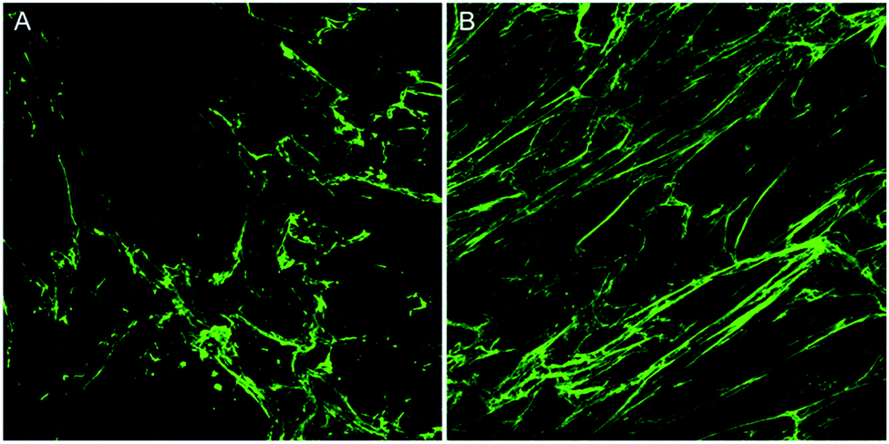 | ||
| Fig. 1 Confocal microscopy image of deposited collagen under ‘crowding’ conditions without and with TGFβ stimulation. (A) Unstimulated control of collagen deposited by human keloid fibroblasts in the scar-in-a-jar model and (B) collagen deposited by human keloid fibroblasts in the scar-in-a-jar model with the addition of TGFβ stimulation. | ||
The standard method for using image analysis to describe orientation can be achieved using the plugin called “Directionality” (http://fiji.sc/User:JeanYvesTinevez), which comes standard in Fiji, an image processing application based on ImageJ.31 This plugin is used to deduce the orientation of structures present in an image. It computes a histogram, which describes the amount of structures in a given direction. This method, as a typical Fourier type analysis, looks for periodic repeats in intensity in the image, generates power spectra and creates a histogram of angular distributions.31 Images with completely isotropic content will give a flat histogram and images that have a preferred orientation are expected to give a histogram with a defined peak at that orientation. The directionality plugin uses Fourier components analysis, based on the Fourier spectrum of an image. For a square image, structures with a preferred orientation generate a periodic pattern at +90° orientation in the Fourier transform of the image, compared to the direction of the objects in the input image. The plugin computes Fourier power spectra of a defined square area in the image. The area is analysed in polar coordinates and the power is measured for each angle using the spatial filters proposed by Liu et al.32 Along with the histogram of angles, the plugin also generates statistics on the highest peak found. To give some quantification for the directionality parameters, the peak is fitted by a Gaussian function, taking into account the periodic nature of the histogram.
In the table of statistics generated, the plugin reports the ‘Direction (°)’, which is the centre of the Gaussian, the ‘Dispersion (°)’, which is the standard deviation of the Gaussian and the ‘Amount’, which is the sum of the histogram from centre − standard deviation to centre + standard deviation, divided by the total sum of the histogram. The true histogram values are used for the summation, not the Gaussian fit. The goodness column reports the fit; 1 is an ideal fit, 0 is the lack of any fit. Using this plugin on test images of deposited collagen, the goodness was always arbitrarily low, which suggests that although the Gaussian is not well suited to the distribution, the plugin recognises this and can quantify to some degree, the uncertainty in the fit. This uncertainty is useful when looking at the ‘dispersion’, which is the standard deviation of the Gaussian peak. In an ideal world, this value could be used to illustrate the angular distribution of an image, and generate a number which would describe the collagen fibrils overall. Unfortunately, this is not the case for images which are not completely uniform, as in the case of most images obtained from a biological environment, and this ‘dispersion’ can be highly misleading. For example, the plugin lacks the ability for multiple peak detection and would therefore pick one peak for the Gaussian and disregard all other peaks. The value for the dispersion then is the standard deviation for the one chosen peak, ignoring the rest of the distribution. It is possible, and was observed with many tested samples, that a narrow Gaussian fit was returned from images that clearly displayed a wide distribution of orientations, which in turn can result in misleading interpretations.
The computed histogram describes the image variation (http://fiji.sc/File:Directionality_Example.png) but is ineffective if statistics on multiple peaks must be generated to return a quantifiable description of the angular distribution. Exporting the data from the table and using various equations to calculate an ‘intensity weighted angular deviation’ does not describe the entire distribution as the exported data is subject to rounding and the image is not well depicted by a sum of angular deviations from a chosen zero angle. A study by Liu et al. revealed that the ‘amount’ value underestimates the real proportion of structures with the preferred orientation.32 Using the pine image as an illustration (http://fiji.sc/File:Directionality_Example.png) it is easy to see that the proportion of needle leaves oriented at +60° is higher than 25%. Because the image is not completely uniform, the meaning of this ‘amount’ value is lost.
Coherency analysis is well suited to the particular structural arrangement present in samples of deposited collagen, because a randomly oriented, basket-weave structure of collagen would correspond to a minimum in coherency. If the collagen angular deviation changes from 90° in any direction, the coherency increases. Thus, this technique is better than the ‘distribution of angle’ analysis that is obtained from the directionality plugin. A perfect basket weave structure would give two distinct angles while a perfectly aligned sample would give only one distinct angle. As biological samples are often not highly uniform, distinguishing between the two would be more difficult than going from a coherence of zero (perpendicular) to a coherence of 1 (parallel). In addition, measuring the standard deviation (distribution) of the fitted orientation distribution curves will give misleading values in a two-peak system, i.e. low angle variation, when in fact it is at its highest variation (perpendicular). The ‘Directionality’ plugin and other similar standard methods of collagen morphology analysis use Fourier transforms which identify gross collagen changes associated with pathological states. However, they are not sufficiently sensitive to measure incremental changes in architecture seen in, for example, the progressive loss of normal architecture with chronological ageing or normal scarring of the skin.
OrientationJ
To overcome the aforementioned drawbacks of the ‘Directionality’ plugin, the ‘OrientationJ’ plugin was explored. It was found that the structure tensor method of image analysis showed a consistent ‘dominant direction’ result as seen with the Fourier analysis method explored with the ‘Directionality’ plugin. Both methods of analysis seem initially suitable for describing the angular distribution within the sample (Fig. 2).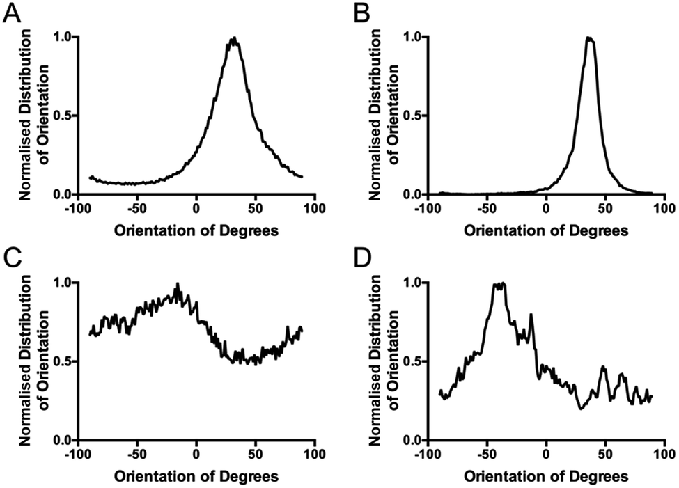 | ||
| Fig. 2 Comparing the computed ‘directionality’ histograms of the unstimulated control and the TGFβ stimulated sample. Computed histograms of: (A) the stimulated control with the directionality plugin, (B) the stimulated control with the coherency analysis in the OrientationJ plugin, (C) the treated sample with the directionality plugin and (D) the treated sample with the coherency analysis in the OrientationJ plugin. | ||
However, the OrientationJ plugin gives a value for coherency without the disadvantages previously discussed involving the Gaussian fit. It can produce a hue-saturation-brightness (HSB) colour map (Fig. 3), similar to the colour survey in the ‘Directionality’ plugin, but the overall coherency value produced when looking at the entire image at once does not work well with large brightness gradients, e.g. non-uniform or sporadic collagen distribution as would be seen as defects in the image. To demonstrate the bias that this overall coherency leads to, images in which there was not a large amount of deposited collagen were analyzed. To solve this image bias, a series of ROI for the plugin to analyze were defined (Fig. 4). The ROIs were made large, so that they were more robust against background noise, as is a feature of structure tensor analysis.33 Because low-resolution structural differences are being observed (i.e. whole fibre variation and not pixel variation with each collagen fibre), the loss in spatial resolution caused by increasing the size of the analysis window in the ROI results in a significant reduction in noise. Additionally, by defining a set number of regions to analyze and taking the average, the likelihood that the measurement for coherency will be skewed one way or the other by spatial variations is reduced.
 | ||
| Fig. 3 Hue, Saturation and Brightness (HSB) maps generated with the OrientationJ plugin. (A) Colour maps of the unstimulated control and (B) the TGFβ stimulated sample. These maps are generated using the OrientationJ plugin, with a particular orientation angle of the collagen assigned to a colour and the saturation of that colour, the local coherency of the image. | ||
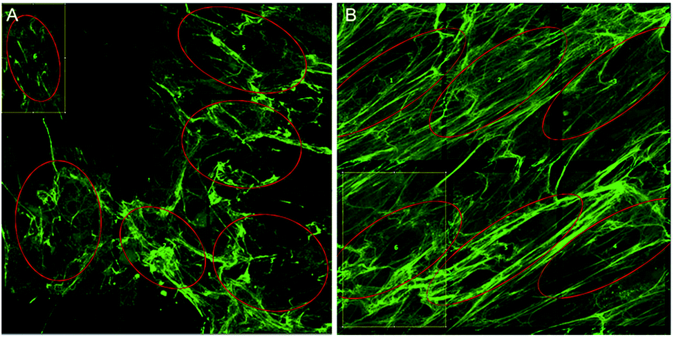 | ||
| Fig. 4 Image region selection used for quantitation. Region of interest (ROI) selection for (A) the unstimulated control and (B) the TGFβ treated sample. Ellipses must be used for structure tensor coherency analysis and the amount of collagen in the ROIs was maximized, avoiding large holes/defects. | ||
User specifics
The structure tensor is a matrix derived from the gradient of a function. It summarizes the predominant directions of the gradient in a specified neighbourhood of a point, and the degree to which those directions are coherent. Within the plugin ‘OrientationJ’ there are a number of different ways to estimate the discrete gradient. As the orientation calculation is only reasonable with a good estimation of the gradient, the plugin allows you to choose between the following gradients: finite difference, Fourier, Gaussian, Riesz filters and cubic spline. The gradients generally have advantages and disadvantages based on their accuracy and time taken to process the function. Finite difference gradient is a poor estimation of the gradient but quite fast because it only looks at the difference between consecutive pixels. Cubic spline makes an exact gradient in the interpolated domain, fast and accurate. Fourier is an exact gradient, but has problems in the periodic boundary conditions that can create image artefacts. Gaussian is a good estimation of image gradient, derived from a truncated version of the Gaussian function. Riesz filters are a low-pass version of the gradient in the Fourier domain which can be useful for reducing image noise. In the plugin author's experience, the cubic-spline gradient is the best trade-off for speed and accuracy. This is the gradient function used in this structure tensor analysis to quantify collagen coherency.Region selection and analysis area
Regions of the samples were imaged by a blinded investigator. The approach was to select representative regions, so a quick scan of the entire samples was performed before regions were chosen. 3 unique and representative regions were selected from each sample, each with an area of 375 by 375 μm. Each sample was experimentally repeated three times. In each image, 6 ROI were selected for coherency analysis (a total of 54 regions for each condition) and the results combined. The areas to be analysed were chosen so as to maximise the amount of collagen area analysed ensuring no overlap between ROIs. Ideally, the entire sample area would be analysed, but due to the design of the in vitro scarring model and the nature of the primary keloid scar fibroblasts, collagen deposition was not uniformly dense across the experimental area. With that in mind, a methodology as described by Kador, et al. (2013) was employed, in that 6 ROI were chosen at random, excluding those areas with deformations or holes.34 The ROIs were kept as large as possible, so as to examine the orientations of the collagen bundles as opposed to the local variations within the bundles (Fig. 4). Pixel coherency can be skewed if the area to be analysed is too small – with no Gaussian smoothing filter, the spatial resolution to noise relationship changes.Images with a low signal to noise ratio can result in the calculated gradient distribution in the random space being affected by local variations in the structure tensor matrix. By expanding the effective radius of the function, the structure tensor is more resistant to background noise, at the cost of diminished spatial resolution.35 This analysis runs into potential problems with biological samples which have a low signal to noise ratio. An example of this is the non-stimulated control samples from the scar in a jar analysis where after 6 days of incubation only a small amount of collagen is deposited, making it difficult to find large regions of representative collagen deposition for coherency analysis. It is therefore inconclusive whether primary dermal scar fibroblasts under non-stimulating conditions will produce collagen as they might in an actual scar (in parallel bundles) or whether they will only produce that scar architecture when in a ‘scar-like’ environment, i.e. stimulated conditions.
Collagen orientation index (COI)
Fourier zeroth-order maximum analysis has been used previously to measure the orientation of collagen fibres.23 Initial attempts to utilise first-order maximum Fourier analysis required substantial observer input, but this approach was refined so that the user selected the region of interest for analysis and a measure of collagen orientation was calculated by determining stretch or elongation of the FFT spectrum.24 Using this method, bundle thickness, spacing and orientation in scar tissue could be compared to normal skin through the use of a Collagen Orientation Index (COI). The COI was developed based on an already existing method of Fourier analysis23 and has been used to compare collagen structure in studies of different scar types, mechanical loading and aging.22,36–38The COI is the ratio of the long axis to the short axis on the ellipse which is calculated from the Fourier transform analysis of an image (Fig. 5). Applying a red-green-blue (RGB) look up table (LUT) to the FFT allowed for clearer definition and measurement of the long and short axis. The elongation of the ellipse is the quantitative measure of the image's alignment. The COI was originally defined as the ‘width/length ratio of the zeroth-order maximum power plot’.23 In most articles though, it is changed to ‘1 – (width/length ratio of the zeroth-order maximum)’. This intuitively appears more logical, with a completely isotropic image resulting in a COI of ‘0’, and a Fourier analysis of an image with perfectly parallel orientation resulting in a COI of ‘1’.19 Normal skin was found to have a significantly lower COI than scar tissue (0.26 versus 0.44, P < 0.001).39 In fact, when compared with normotrophic, hypertrophic and keloid scars, normal skin had a significantly lower COI, which indicates that collagen in all types of scars is organised in a more parallel nature.40 The results of COI analysis were compared to the developed coherency analysis on the example images for this study (Fig. 6).
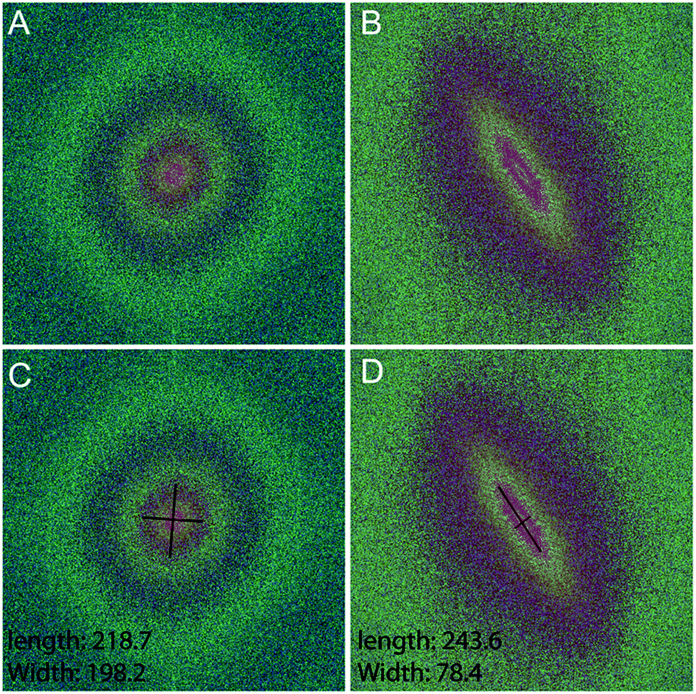 | ||
| Fig. 5 Testing the COI technique with Fourier analysis of the test images. Fast Fourier Transforms (FFTs) with an RGB LUT applied of (A) the unstimulated control and (B) the TGFβ treated sample. The corresponding measurement of the length and width of the FFT ellipses are shown for (C) the unstimulated control and (D) the TGFβ treated sample. | ||
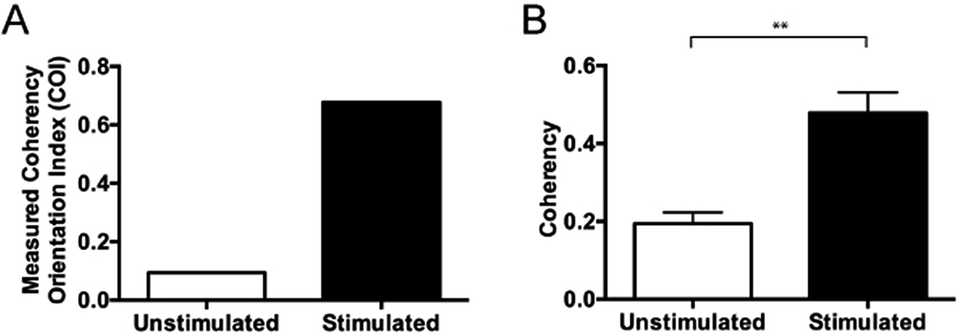 | ||
| Fig. 6 Comparing coherency analysis with COI analysis. (A) COI analysis of both the unstimulated control and the TGFβ treated sample and (B) coherency analysis of both the unstimulated control and the TGFβ treated sample. As the COI measurement is a function of the entire sample, the difference cannot be statistically quantified, but with the multiple sampling of the image with coherency analysis, the difference can be statistically agreed upon (**p < 0.0001), data displayed as mean ± SD and statistically assessed with a one-way ANOVA followed by a Bonferroni comparison test. | ||
Preliminary studies with Dupuytren scar cells reinforce that this technique remains suitable for these cell types also. Measured coherency shows a significant increase after the same TGFβ stimulation that was tested with this methodology (Fig. 7). This is especially relevant because of the way in which keloid and Dupuytren cells deposit collagen compared to ‘normal’ dermal scar fibroblasts. Keloid cells, for example, deposit collagen in tightly packed dense bundles. They also form acellular nodes of collagen parallel to the skin surface and have a much more aggressive pathology than normal scar fibroblasts.41 Dupuytren's disease is characterized by a dense, highly organized collagen matrix which orients longitudinally and contains nodules and myofibroblasts aggregates.42 This data shows that the computational quantitation works for highly variant amounts of collagen. It adds to the robustness of the technique as a tool for collagen assessment in a range of scar scenarios.
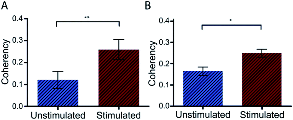 | ||
| Fig. 7 Coherency analysis on keloid and Dupuytren scar cells. Unstimulated and TGFβ stimulated (A) keloid and (B) Dupuytren cells were compared with this method of coherency analysis and found to be significantly different. This demonstrates the robustness of the methodology for analysing an assortment of scar cells with varying amounts of deposited collagen, i.e. large excesses of collagen as produced by stimulated keloid and Dupuytren cells. Dupuytren n = 4, *p < 0.001. Keloid n = 6, **p < 0.0001, data displayed as mean ± SD and statistically assessed with a one-way ANOVA followed by a Bonferroni comparison test. | ||
Further to the in vitro assessment, coherency analysis was also possible in comparing sections of normal skin tissue with that of scar and tendon. Here the coherency analysis was applied to the entirety of ten individual images of each tissue type and compared. It is well documented that tendon consists of aligned and tightly packed parallel bundles of collagen fibres. It is this architecture, which promotes high strength in the tissue along the direction of fibre alignment.43 Similarly, the effects of scarring on skin architecture is similar to that presented earlier where we see a deviation to more striated collagen architecture from the normal random orientation of healthy skin. In comparing the coherency analysis with images taken from rat tendon to that of normal rat skin a significant increase in the measured coherency is evident (Fig. 8).
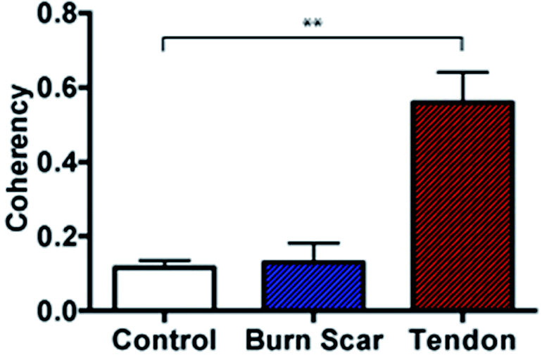 | ||
| Fig. 8 Coherency analysis on rat tissue sections. Coherency analysis comparing control skin with scar following a burn injury to that of rat tendon. The collagen fibre alignment in tendon is significantly different to that of control skin however there was no significant difference evident when comparing control skin with normal scarring in the rat, n = 10 images per sample, **p < 0.0001, data displayed as mean ± SD and statistically assessed with a one-way ANOVA followed by a Bonferroni comparison test. | ||
In comparing the orientation of the scar to normal skin there was no significant difference observed. This however is not surprising with the impressive healing abilities of rats compared with humans, leaving little scar type tissue to assess and minimal changes to structure. Recent studies by Quinn et al. were in fact able to detect collagen architecture differences using a directional statistics method in a similar full thickness contact burn injury model in rats. However, these differences were only detected at time points beyond 2 months compared to this study where tissue was collected earlier (at 3 weeks post injury) for analysis and in turn also unable to detect significant changes at this early time point.25 It is anticipated that the use of porcine tissue as an in vivo model will provide measurable differences in the collagen architecture and similarly that these differences can be seen in human tissue samples as well as in more mature scars as seen in previous studies.25
Finally to investigate inter and intra-rater variability with the technique 2 blinded assessors were provided with 18 de-identified immunohistochemically stained images of TGFβ stimulated primary normotrophic collagen architecture similar to those as the focus in this study. They also analysed 50 images from human skin sections using the same approach. Rater 1 repeated the process twice while rater 2 only once to provide intra and inter-rater comparisons respectively. It was found that there was no significant difference in the measured coherency analysis of either the in vitro images or the images of rat skin sections (see ESI,† Fig. 1) further supporting the robustness of this technique.
Conclusions
In summary, coherency analysis using this method is a novel approach to objectively quantify collagen morphology. Collagen produced by primary keloid scar cells in a scar-like environment was used as a research model for demonstrating this technique. Our data illustrates that coherency analysis based on structure tensors is a sensitive, reproducible technique that can be used to provide quantification of collagen orientation and thus scar quality. This technique has been shown to be more suitable than methods involving Fourier analysis and consistently gives more representative and results with higher resolution. Further to this, validation in tissue sections provides evidence for this technique being suitable for assessment of scar outcome and future work will look to analyse human hypertrophic and keloid scar samples with this method. This technique will serve as a research tool to explore the pathogenesis of scar development and will be especially critical in the development of new strategies to combat excessive collagen deposition in scarring and therapies, which target the morphology of the deposited collagen.Conflicts of interest
The authors declare that there are no conflicts of interest.Acknowledgements
The authors acknowledge the Australian Microscopy & Microanalysis Research Facility at the Centre for Microscopy, Characterization & Analysis, The University of Western Australia, funded by the University, State and Commonwealth Governments. The authors would like to acknowledge Dr Christian Couppé and Dr Peter Schjerling, Institute of Sports Medicine/IOC Research Center Copenhagen, Center for Injury Prevention and Protection of Athlete Health, Bispebjerg Hospital, Denmark for supplying the rat tendon images used in this study and Dr Darragh K. Waters from the Royal College of Surgeons of Ireland, Dublin, Ireland and Dr Laura Caul from Fiona Stanley Hospital, Perth, Australia for their help in comparing inter and intra-rater reliability of the coherency measurement. This work was supported by the Australian Research Council (ARC) Linkage Grant, Discovery Project & National Health and Medical Research Council (NHMRC) grants awarded to Dr T. Clemons, W/Prof. F. Wood, Dr M. W. Fear and Prof. K. S. Iyer.References
- P. Durani, D. McGrouther and M. Ferguson, J. Plast. Reconstr. Aesthet. Surg., 2009, 62, 713–720 CrossRef PubMed.
- P. Van Zuijlen, A. P. Angeles, R. W. Kreis, K. E. Bos and E. Middelkoop, Plast. Reconstr. Surg., 2002, 109, 1108–1122 CrossRef PubMed.
- C. Roques and L. Teot, Int. J. Lower Extremity Wounds, 2007, 6, 249–253 CrossRef CAS PubMed.
- P. S. Powers, S. Sarkar, D. B. Goldgof, C. W. Cruse and L. V. Tsap, J. Burn Care Res., 1999, 20, 54–60 CrossRef CAS.
- N. Idriss and H. I. Maibach, Skin Res. Technol., 2009, 15, 1–5 CrossRef PubMed.
- M. J. Baryza and G. A. Baryza, J. Burn Care Res., 1995, 16, 535–538 CrossRef CAS.
- N. Brusselaers, A. Pirayesh, H. Hoeksema, J. Verbelen, S. Blot and S. Monstrey, J. Surg. Res., 2010, 164, e115–e123 CrossRef PubMed.
- O. Bock, G. Schmid-Ott, P. Malewski and U. Mrowietz, Arch. Dermatol. Res., 2006, 297, 433–438 CrossRef PubMed.
- M. B. van der Wal, P. D. Verhaegen, E. Middelkoop and P. P. van Zuijlen, J. Burn Care Res., 2012, 33, e79–e87 CrossRef CAS PubMed.
- R. Fearmonti, J. Bond, D. Erdmann and H. Levinson, ePlasty, 2010, 10, 354–363 Search PubMed.
- M. Masters, M. McMahon and B. Svens, J. Burn Care Res., 2005, 26, 273–284 Search PubMed.
- L. Forbes-Duchart, S. Marshall, A. Strock and J. E. Cooper, J. Burn Care Res., 2007, 28, 460–467 CrossRef PubMed.
- P. Whittaker, R. Kloner, D. Boughner and J. Pickering, Basic Res. Cardiol., 1994, 89, 397–410 CrossRef CAS PubMed.
- L. C. Junqueira, G. Bignolas and R. Brentani, Histochem. J., 1979, 11, 447–455 CrossRef CAS PubMed.
- H. Khorasani, Z. Zheng, C. Nguyen, J. Zara, X. Zhang, J. Wang, K. Ting and C. Soo, Am. J. Pathol., 2011, 178, 621–628 CrossRef PubMed.
- D. Guidolin, A. Vacca, G. G. Nussdorfer and D. Ribatti, Microvasc. Res., 2004, 67, 117–124 CrossRef CAS PubMed.
- J. P. Tinajero, R. Robledo, R. C. Lantz, R. E. Sobonya, S. F. Quan, R. J. Lemen, B. J. Tollinger and M. L. Witten, Res. Commun. Mol. Pathol. Pharmacol., 1997, 95, 275–285 CAS.
- A. Eblen-Zajjur, R. Salas and H. Vanegas, Comput. Biol. Med., 1996, 26, 87–95 CrossRef CAS PubMed.
- P. P. van Zuijlen, H. J. de Vries, E. N. Lamme, J. E. Coppens, J. van Marle, R. W. Kreis and E. Middelkoop, J. Pathol., 2002, 198, 284–291 CrossRef PubMed.
- P. P. van Zuijlen, E. N. Lamme, M. J. van Galen, J. van Marle, R. W. Kreis and E. Middelkoop, Burns, 2002, 28, 151–160 CrossRef PubMed.
- C.-I. Chang, IEEE Trans. Inf. Theory, 2000, 46, 1927–1932 CrossRef.
- S. Wu, H. Li, H. Yang, X. Zhang, Z. Li and S. Xu, J. Biomed. Opt., 2011, 16, 040502–040503 CrossRef PubMed.
- H. J. de Vries, D. N. Enomoto, J. van Marle, P. P. van Zuijlen, J. R. Mekkes and J. D. Bos, Lab. Invest., 2000, 80, 1281–1289 CrossRef CAS PubMed.
- P. D. Verhaegen, J. Van Marle, A. Kuehne, H. J. Schouten, E. A. Gaffney, P. K. Maini, E. Middelkoop and P. P. Van Zuijlen, J. Microsc., 2012, 245, 82–89 CrossRef PubMed.
- K. P. Quinn, A. Golberg, G. F. Broelsch, S. Khan, M. Villiger, B. Bouma, W. G. Austen, R. L. Sheridan, M. C. Mihm and M. L. Yarmush, Exp. Dermatol., 2014, 23 Search PubMed.
- C. Z. Chen, Y. X. Peng, Z. B. Wang, P. V. Fish, J. L. Kaar, R. R. Koepsel, A. J. Russell, R. R. Lareu and M. Raghunath, Br. J. Pharmacol., 2009, 158, 1196–1209 CrossRef CAS PubMed.
- C. Couppe, R. B. Svensson, K. M. Heinemeier, E. W. Thomsen, M. L. Bayer, L. Christensen, M. Kjaer, S. P. Magnusson and P. Schjerling, Histochem. Cell Biol., 2017, 147, 97–102 CrossRef CAS PubMed.
- R. Rezakhaniha, A. Agianniotis, J. T. C. Schrauwen, A. Griffa, D. Sage, C. Bouten, F. Van de Vosse, M. Unser and N. Stergiopulos, Biomech. Model. Mechanobiol., 2012, 11, 461–473 CrossRef CAS PubMed.
- E. Fonck, G. G. Feigl, J. Fasel, D. Sage, M. Unser, D. A. Rüfenacht and N. Stergiopulos, Stroke, 2009, 40, 2552–2556 CrossRef CAS PubMed.
- J. Hertz, R. Robinson, D. A. Valenzuela, E. B. Lavik and J. L. Goldberg, Acta Biomater., 2013, 9, 7622–7629 CrossRef CAS PubMed.
- C. A. Schneider, W. S. Rasband and K. W. Eliceiri, Nat. Methods, 2012, 9, 671–675 CrossRef CAS PubMed.
- Z.-Q. Liu, Appl. Opt., 1991, 30, 1369–1373 CrossRef CAS PubMed.
- Z. Ding, J. C. Gore and A. W. Anderson, Magn. Reson. Med., 2005, 53, 485–490 CrossRef PubMed.
- K. E. Kador, R. B. Montero, P. Venugopalan, J. Hertz, A. N. Zindell, D. A. Valenzuela, M. S. Uddin, E. B. Lavik, K. J. Muller and F. M. Andreopoulos, Biomaterials, 2013, 34, 4242–4250 CrossRef CAS PubMed.
- G. Medioni, M.-S. Lee and C.-K. Tang, A computational framework for segmentation and grouping, Elsevier, University of South California, Los Angeles, USA, 2000 Search PubMed.
- X. Jiang, S. Chen, J. Chen, X. Zhu, L. Zheng, S. Zhuo and D. Wang, Laser Phys., 2011, 21, 1661–1664 CrossRef CAS.
- X. Zhu, S. Zhuo, L. Zheng, K. Lu, X. Jiang, J. Chen and B. Lin, J. Biophotonics, 2010, 3, 108–116 CrossRef CAS PubMed.
- P. D. Verhaegen, H. J. Schouten, W. Tigchelaar-Gutter, J. Marle, C. J. Noorden, E. Middelkoop and P. P. Zuijlen, Wound Repair Regen., 2012, 20, 658–666 CrossRef PubMed.
- P. P. van Zuijlen, J. J. Ruurda, H. A. van Veen, J. van Marle, A. J. van Trier, F. Groenevelt, R. W. Kreis and E. Middelkoop, Burns, 2003, 29, 423–431 CrossRef PubMed.
- P. D. Verhaegen, P. P. Van Zuijlen, N. M. Pennings, J. Van Marle, F. B. Niessen, C. M. Van Der Horst and E. Middelkoop, Wound Repair Regen., 2009, 17, 649–656 CrossRef PubMed.
- A. S. Halim, A. Emami, I. Salahshourifar and T. P. Kannan, Arch. Plast. Surg., 2012, 39, 184–189 CrossRef PubMed.
- R. Mafi, S. Hindocha and W. Khan, Open Orthop. J., 2012, 6, 77 CrossRef PubMed.
- B. K. Connizzo, S. M. Yannascoli and L. J. Soslowsky, Matrix Biol., 2013, 32, 106–116 CrossRef CAS PubMed.
Footnote |
| † Electronic supplementary information (ESI) available: Table comparing collagen quantification techniques following a burn injury as well as comparison of inter and intra-rater reliability of the coherency analysis provided. See DOI: 10.1039/c7ra12693j |
| This journal is © The Royal Society of Chemistry 2018 |