
 Open Access Article
 This Open Access Article is licensed under a Creative Commons Attribution-Non Commercial 3.0 Unported Licence
Is soft independent modeling of class analogies a reasonable choice for supervised pattern recognition?†
Anita Rácz a,
Attila Gereb,
Dávid Bajuszc and
Károly Héberger*a
a,
Attila Gereb,
Dávid Bajuszc and
Károly Héberger*a
aPlasma Chemistry Research Group, Research Centre for Natural Sciences, Hungarian Academy of Sciences, Magyar tudósok krt. 2, H-1117 Budapest, Hungary. E-mail: heberger.karoly@ttk.mta.hu
bSzent István University, Faculty of Food Science, Sensory Laboratory, Villányi út 29-43, H-1118 Budapest, Hungary
cMedicinal Chemistry Research Group, Research Centre for Natural Sciences, Hungarian Academy of Sciences, Magyar tudósok krt. 2, H-1117 Budapest, Hungary
First published on 20th December 2017
Abstract
A thorough survey of classification data sets and a rigorous comparison of classification methods clearly show the unambiguous superiority of other techniques over soft independent modeling of class analogies (SIMCA) in the case of classification – which is a frequent area of usage for SIMCA, even though it is a class modeling (one class or disjoint class modeling technique). Two non-parametric methods, sum of ranking differences (SRD) and the generalized pairwise correlation method (GPCM) have been used to rank and group the classifiers obtained from six case studies. Both techniques need a supervisor (a reference) and their results support and validate each other, despite being based on entirely different principles and calculation procedures. To eliminate the effect of the chosen reference, comparisons with one variable (classifier) at a time were calculated and presented as heatmaps. Six case studies show unambiguously that SIMCA is inferior to other classification techniques such as linear and quadratic discriminant analyses, multivariate range modeling, etc. This analysis is similar to meta-analyses frequently applied in medical science nowadays; with the notable difference that we did not (and should not) make any distributional assumptions. A well-founded conclusion can be drawn, as we could not find any circumstances when SIMCA is superior to concurrent techniques. Hence, the question in the title is self-explanatory.
1. Introduction
Supervised and unsupervised pattern recognition techniques are two of the largest and most frequently-used branches of chemometric methods. Supervised pattern recognition (or classification) relies on a grouping variable (class membership information) to estimate and assign class memberships, while unsupervised techniques work without this information to find dominant patterns and outliers in the model or dataset.The most frequently used pattern recognition technique is in all probability principal component analysis (PCA),1 which is a straightforward and powerful tool of chemometricians. One can find thousands of publications in many fields of science, which utilize the dimension reduction ability of PCA. On the other hand, there are plenty of extensions of PCA, for example, successive PCA, prioritized PCA, or independent component analysis (ICA). Also, the well-known soft independent modeling of class analogies (SIMCA) can be considered as such an extension.
Soft independent modeling of class analogies (SIMCA) has been frequently used as a supervised pattern recognition method in the field of chemometrics in the past decades. However, SIMCA is a class-modeling technique; it is based on disjoint principal component analyses: applying one PCA for each class of the whole dataset. SIMCA was first introduced by Wold2 and since then, several applications have followed. SIMCA performs a PCA on each of the predefined classes from the training set. The optimum number of principal components (PCs) may be pre-defined, chosen based on explained variance or determined by (double) cross-validation.
Prior to modeling, mean centering is applied and the new cases are fitted to the model. The average orthogonal distance (residual standard deviation, RSD) of the new case is computed from each class. The orthogonal distance (OD) represents the Euclidean distance of an observation to the PCA subspace of the given class.3 “The critical RSD value RSDcrit, i.e., the border of the model, is calculated, where RSDref is the mean residual standard deviation of the reference samples. Fcrit is the F value at the selected level of significance and the proper degrees of freedom.
| RSDcrit = RSDref × Fcrit |
Whether or not sample i belongs to the modeled class can be determined by comparing RSDi and RSDcrit. The ratio between these values corresponds to the degree of similarity. If the ratio is lower than 1.0, sample i belongs to the model and if it is higher, the sample does not belong to the model.”4
Ultimately, this means that SIMCA focuses more on the similarities among samples within a class than on the differences between the classes.5
SIMCA is a flexible method and gives further information about the class memberships. Several options should be considered prior to modeling: scaling of the variables, way of determining the number of PCs, number of PCs, expanded or contracted range, different weights for the distances from the model in the inner space and in the outer space, weighting of the variables after class-autoscaling, etc.6
In spite of its popularity, several papers have demonstrated the poor performance of SIMCA as compared to other methods, e.g. to linear discriminant analysis (LDA). The fact that LDA was developed by statisticians, whereas SIMCA was developed by chemists (chemometricians) might contribute to the characteristic differences between their theoretical backgrounds. For example, SIMCA does not require any distributional assumptions, whereas LDA assumes normal distribution and equal variances for each class. Also, LDA forces to classify all samples in one of the classes, while SIMCA can differentiate in-class and out-of-class situations for each class independently: if a sample is assigned to none of the classes, a new class may be found and defined. The main advantage of SIMCA comes from its feature that the model is created for a given category and it returns whether a sample belongs to that category or not.5 Moreover, SIMCA allows classifying a sample into multiple classes.
Regularized discriminant analyses use a meta-parameter to develop a better estimate of the covariance matrix of the data than linear or quadratic discriminant analysis without ignoring the differences in the covariance that may be present in the data.7
The best-known example of regularized discriminants is SIMCA. Although discriminant analysis methods can operate with various types of class boundaries (e.g. linear for LDA or quadratic for QDA), SIMCA is a definite exception and, as we will see later, its performance does not correspond to the expectations.
Despite several articles showing the poor performance of SIMCA for classification tasks, numerous applications can be found in the literature. Moreover, based on a Scopus search, the number of publications is increasing rapidly in the past twenty years, which can be clearly seen in Fig. 1. Based on our findings about the frequent use of SIMCA, the aim of our paper is to conduct a meta-analysis using the results of six published papers in order to evaluate the performance of SIMCA, to compare it with other classification methods, and to unravel, whether SIMCA is inferior to discriminant analysis methods or not.
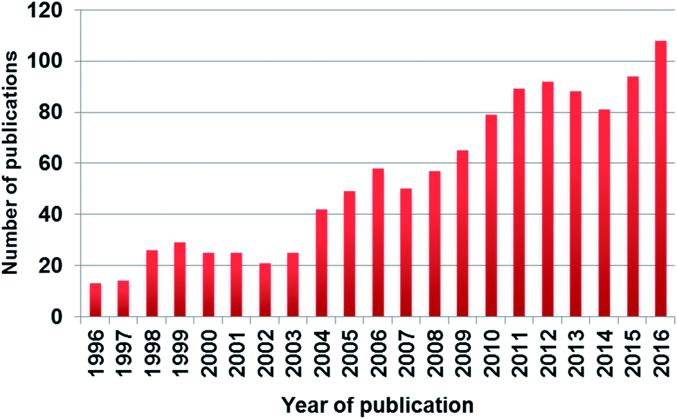 | ||
| Fig. 1 The number of published papers in the past twenty years based on Scopus search with keywords “SIMCA” or “soft independent modeling of class analogies”. | ||
Our secondary aim is to highlight that SIMCA was created primarily as a class-modeling method, and although it can be used as a discriminant tool, proper performance measurements are needed. We propose a methodology which fulfills this goal and is able to assess the performance of multiple discriminant methods on the same data set.
We emphasize that – consistently with the practice of meta-analyses – we do not deal with simulated or aggregated data, to avoid the biases coming from individual analyses. The real performance of the methods is evaluated on the original, published data sets because this way higher statistical power is achieved and our results become more robust.
2. Methods
2.1 Sum of ranking differences
Sum of ranking differences (SRD) is a basic and simple tool for ranking methods or models in every field of science,8 introduced in the work of Héberger.9 Its basic principle is the following: first, a data matrix is formed, where the columns contain the information we want to compare (e.g. methods, models) and the rows contain the data instances (samples, objects, etc.). Next, we have to define a reference column, which can be an “exact golden reference” or the average, minimum, maximum, etc. This is really important, as the data values in each column are ranked by increasing magnitude and these rankings are compared to the ranks of the reference column. Finally, the absolute differences between the rank-variables and the rank-reference columns in each case are calculated and summed. These values (SRD values) give us the ordering of the variables. The smaller the SRD value, the better (or the more consistent) the variable is. The procedure above is explained in detail in one of our recent works.10The SRD procedure applies two validation approaches: first, the calculation is repeated many times with the use of random numbers and the frequency distribution of the SRD values across these calculations is plotted along with the actual results. This usually gives a Gaussian curve: if a method has an SRD value that overlaps with this curve, its ranking behavior cannot be considered to be significantly different from random ranking. Second, a suitable cross-validation approach (sevenfold cross-validation with 14 or more samples and leave-one-out cross-validation with 13 or fewer samples) can be applied to retrieve an SRD value distribution for each of the compared methods. It can be established whether two methods provide significantly different results, with the use of a parametric or a non-parametric statistical test. The choice for cross-validation is supported by our recent work.11 The nonparametric sign test12 and Wilcoxon test,13 as well as Student's t-test are used to compare the cross-validated SRD values to decide whether the methods are significantly different. Nonparametric tests were computed using Statistica v.10 (StatSoft, Tulsa, Oklahoma, USA). An extension of the basic method was published last year, to address the question of reference selection. In a new approach, termed COVAT (comparison with one variable at a time), we use each available variable as the reference exactly once and present the results in a heatmap format. We have shown that this approach can increase the “resolution” of SRD calculations (e.g. variables whose SRD values did not differ significantly in the original SRD calculation can be differentiated in many cases) and provides more discriminatory power than the application of parametric and non-parametric correlation coefficients.14 SRD has been successfully applied for calibration,15 selecting performance parameters, model updating, residual penalties,16 as well as for bias-variance tradeoffs.17
2.2 Generalized pairwise correlation method
The generalized pairwise correlation method (GPCM) is based on a 2 × 2 contingency matrix, which counts the frequencies of four events: A, B, C, and D. The frequencies are calculated from comparisons between each possible variable pair (X1 and X2) and the reference variable (Y) for every possible pair of objects. In this study, arithmetic mean was used as the reference variable. Event A occurs when the given pair of objects strengthens the correlation for both of the compared variables (i.e. if Yi > Yj, than X1i > X1j and X2i > X2j). Similarly, event D occurs when the pair of objects weakens the correlation of both compared variables with the Y variable (i.e. if Yi > Yj, than X1i < X1j and X2i < X2j). Events B and C are complementary: the correlation is strengthened for variable X1 and weakened for X2 (event B) and vice versa (event C).18The final decision of the comparison between variable pairs is based on conditional Fisher's exact test or McNemar's test. The procedure is repeated for every possible variable pair. A variable can win the final comparison if it has the most “win” decisions. ”No decision” results mean that there is no significant difference between the correlations of the reference variable and the members of the pair. GPCM compares all the different variable pairs, and counts “wins”, “losses” and “no decisions (ties)” between the variables. The final results can be presented in three different ways: simple ordering by the number of wins, difference ordering (by the differences between the number of wins and losses), and significance ordering (probability-weighted version of difference ordering).18
A great advantage of SRD and GPCM is that they are able to compare (order, group) biased estimations as well. The biases of various methods (techniques, labs, operators, etc.) follow normal distribution, similarly to the random errors. Hence, the proposed approach is sufficient for the comparison of highly different methods using their performance parameters.
3. Results
Six case studies were used for the comparison of the different classifier methods. The specific details about the studies and the applied data matrices can be found in the ESI Table 1.† In the following section, the results of each study are discussed separately.3.1 Case study 1
Todeschini et al. compared various frequently used classifiers based on their performance on 27 emblematic data sets.19 Table 5 of their paper contains leave-one-out non-error rates (NER%) obtained for the 27 data sets by the selected classification methods. (NER% is identical to the correct classification rate, CC%.)Todeschini et al. have introduced two new classifiers (D-CAIMAN and M-CAIMAN) and compared their performances with well-known classifiers, such as linear discriminant analysis (LDA), quadratic discriminant analysis (QDA), k-nearest neighbors (KNN), classification and regression trees (CART), nearest mean classifier (NMC), unequal dispersed classes (UNEQ) and SIMCA. They have also carried out a principal component analysis including two theoretical methods: the method “WORST”, constituted by the worst obtained result for each data set and the method “BEST”, constituted by the best-obtained result for each data set. The first principal component (PC1) gives the WORST–BEST direction, explaining more than 50% of the total variance: this component is related to the overall quality of the methods. The second component (PC2) is related to the alternative behavior of CART, LDA, and NMC, which give very good results for some data sets and very poor results for other data sets.19
SRD as a fair method comparison technique fully supports Todeschini et al.'s conclusions: while the evaluation is simplified into one dimension, the BEST (Max) and WORST relation (Min) is preserved, see Fig. 2.
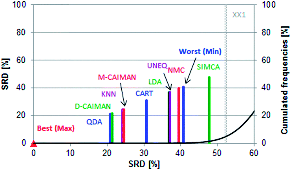 | ||
| Fig. 2 Normalized SRD values (between 0 and 100) compared to random ranking (increasing part of the black cumulative distribution function (CDF) curve) for the non-error rates (NER%) of 27 data sets. Scaled SRD values are plotted on the x and left y-axes, the right y-axis shows the cumulated relative frequencies for random ranking (black curve). The 5% probability level (XX1) is also given. | ||
Row maxima were used as the reference (benchmark) column, as they provide a hypothetical best method. In this example, none of the methods overlap with the Gaussian curve, thus all of them are significantly different from random ranking. The best possible ranking is at SRD(Max) = 0, while the hypothetical worst classification has an SRDnormalized value of 40.66. Interestingly, SIMCA provides an even worse ranking (SRDnormalized = 47.802), which is still significantly different from random ranking at the 5% level according to the Wilcoxon matched pair test (sevenfold cross-validation).
The best position of QDA is understandable, as some of the datasets are linearly not separable; the intermediate position of LDA can be explained with the same argumentation. D- and M-CAIMAN are among the best representations, supporting the suggestion of Todeschini et al.19 Furthermore, the conclusion that D-CAIMAN (discriminative CAIMAN) performs better than M-CAIMAN (modeling CAIMAN) is consistent with the original (although implicit) conclusion of the authors, see Fig. 3. UNEQ's resemblance to QDA is not observed, probably because the initial assumptions are not met (“UNEQ can be applied when only a few variables must be considered”20).
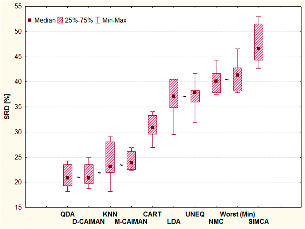 | ||
| Fig. 3 Sevenfold cross-validated SRD results for the nine classifiers.19 The best result (SRD = 0) achieved with the row-maxima as reference is omitted for clarity. The symbol “∼” means no significant difference at the 5% level according to the Wilcoxon matched pair test. | ||
Sevenfold cross-validation (leaving out contiguous blocks21) allows the rendering of uncertainties to any single SRD value. The pairwise Wilcoxon matched pairs test is suitable to establish whether a significant difference exists among two methods.
The results of this case study are presented as sevenfold cross-validated SRD values in Fig. 3. The ordering is self-explanatory; UNEQ and LDA have some common features (assumption of normality), which explains their proximity in the SRD ordering. A certain grouping is instantly recognizable: I (QDA, D-CAIMAN, M-CAIMAN, KNN), II (CART), III (LDA, UNEQ, NMC, WORST), and IV (SIMCA). SIMCA is not only the last ranked method; it is significantly worse than the worst option (Min), i.e. reversely ranked partly. Moreover, it has the largest variance.
One may argue, however, that SRD ranking greatly depends on the selected reference, which is indeed an inherent feature of the method. Although a hypothetical best method comprising the best individual performances for 27 datasets is a natural choice, we examined other choices for the reference: with the SRD-COVAT approach, all method performances (NER%) were used as the reference exactly once.14 The result of SRD-COVAT is presented in Fig. 4.
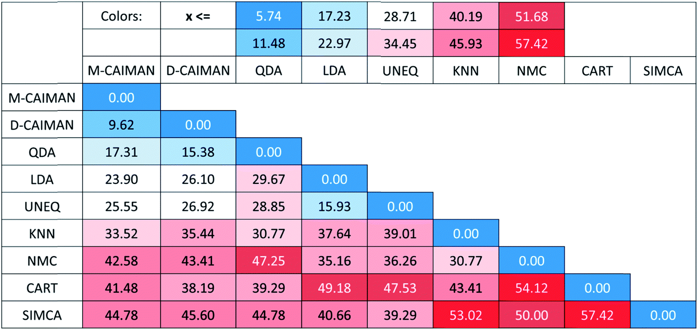 | ||
| Fig. 4 Heatmap representation of the SRD-COVAT matrix for Case study 1. SRD values increase in the blue (highest similarity) towards red (lowest similarity) direction. The classifiers are enumerated in the order of increasing sums of SRD values. Color codes are provided in the header with relative (%) values. | ||
A somewhat different pattern is visible on the heatmap than in the previous figures. The maximum and minimum as reference distinguish evidently two clusters: I (D-CAIMAN, M-CAIMAN, QDA), and II (LDA, UNEQ). An interesting conclusion can be drawn for the KNN method: while its distance from the row maximum (or BEST method) is similar to those of D-CAIMAN, M-CAIMAN, and QDA, it does not belong to the same cluster as these three methods. (Being based on a rather different principle, this is not surprising.) This clustering clearly assigns a recommendation order: techniques in Cluster I are suggested to be applied in various and problematic cases such as the 27 datasets; cluster II may be recommended in special cases only (however, the specificity of the datasets is rarely known before an analysis), and the rest of the techniques are not recommended by default.
GPCM fully supports the previous findings, which can be seen in Table 2 in the ESI.† The ordering corresponds to the expectations, QDA and D-CAIMAN are the best and the first four techniques are clearly distinguished from the remaining ones. CART has an intermediate position with 3 wins and 2 losses (see also Fig. 3, 4, 7 and 8 in the original work19). NMC and SIMCA could not be superior to any of the techniques examined, and SIMCA was outperformed even by NMC.
3.2 Case study 2
Tax in his Ph.D. work, when introducing one-class classification, compares several classification techniques using 13 data sets complemented with outlying observations.22 His Table 2.2 has been completed with row minima and row maxima and submitted to a ranking procedure with sum of ranking differences.Table 2.2 in ref. 22 contains classification errors of some conventional classifiers and some one-class classifiers (trained on each class separately). The examined conventional classifiers include a linear classifier based on normal densities (Bayes), a Parzen classifier and a support vector classifier with a third degree polynomial kernel (SVC-p3). In addition, four versions of the support vector data description (SVDD) classifier were introduced and examined as novel one-class classifiers, (hence, in this case study not SIMCA, but one-class classifiers are discussed). These include SVDD with a third degree polynomial kernel (SVDD-p3), SVDD with a Gaussian kernel (simply referred to as SVDD), and the counterparts of these methods where negative examples were utilized during the training (SVDD-neg and SVDD-n-p3). When the polynomial kernel was used, the data are rescaled to unit variance.
Among others, Tax concludes that conventional classifiers (especially Parzen and SVC-p3) outperform SVDD in most cases and that the performance of SVDD is better with the inclusion of example outliers and with the Gaussian kernel.
In the case of such ambiguous outcomes, method comparison based on sum of ranking differences is an advantageous choice. The ordering and ranking of the classifiers can be seen in Fig. 5. The row minima were used as the reference: for error rates, this constitutes a similar, hypothetical best method as in the previous case study.
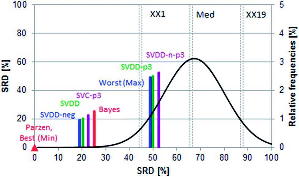 | ||
| Fig. 5 Normalized SRD values (between 0 and 100) compared to random ranking (black Gaussian curve) for the error rates (ER%) of 13 data sets. Row minima were used as the reference. Best (Min) and Worst (Max) denote row minima and maxima, respectively. Scaled SRD values are plotted on the x and left y-axes, while the right y-axis shows the relative frequencies for the black curve. The 5% probability level (XX1), median (Med) and 95% level (XX19) are also given for the “random” distribution. | ||
Fig. 6 shows that all methods are significantly different according to the t-test, sign test, and Wilcoxon matched pair test, except one pair (SVDD-neg and SVDD denoted by “∼”). Although the ordering of classical and SIMCA-like one-class classifiers is dispersed and overlapping, the best method is a classical one (Parzen) and only the two one-class methods (SVDD-p3 and SVDD-n-p3) are not distinguishable from random ranking. In fact, they are significantly worse than the row maxima (hypothetical worst case).
 | ||
| Fig. 6 Sevenfold cross-validated SRD results for eight classifiers. The best results (SRD = 0), achieved with the row minima as reference, belong to the Parzen classifier. The symbol “∼” means no significant difference at the 5% level according to the Wilcoxon matched pair test. | ||
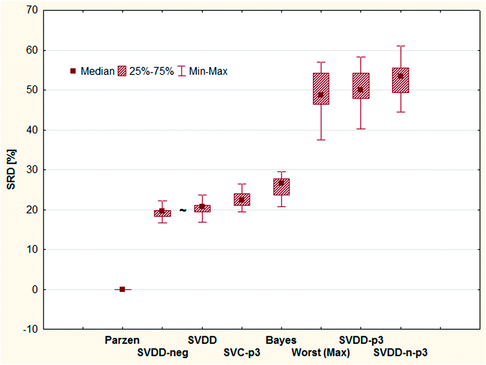
Although the reference vector, the row minimum is the natural choice to keep the errors minimum, one may argue with the decisive role of the reference vector in the above examinations. Therefore, we completed an SRD-COVAT calculation for this dataset as well. Since the objects are ranked according to decreasing magnitude during the SRD calculations, we have taken the (1-error) values in our input matrix. The result is given in Fig. 7.
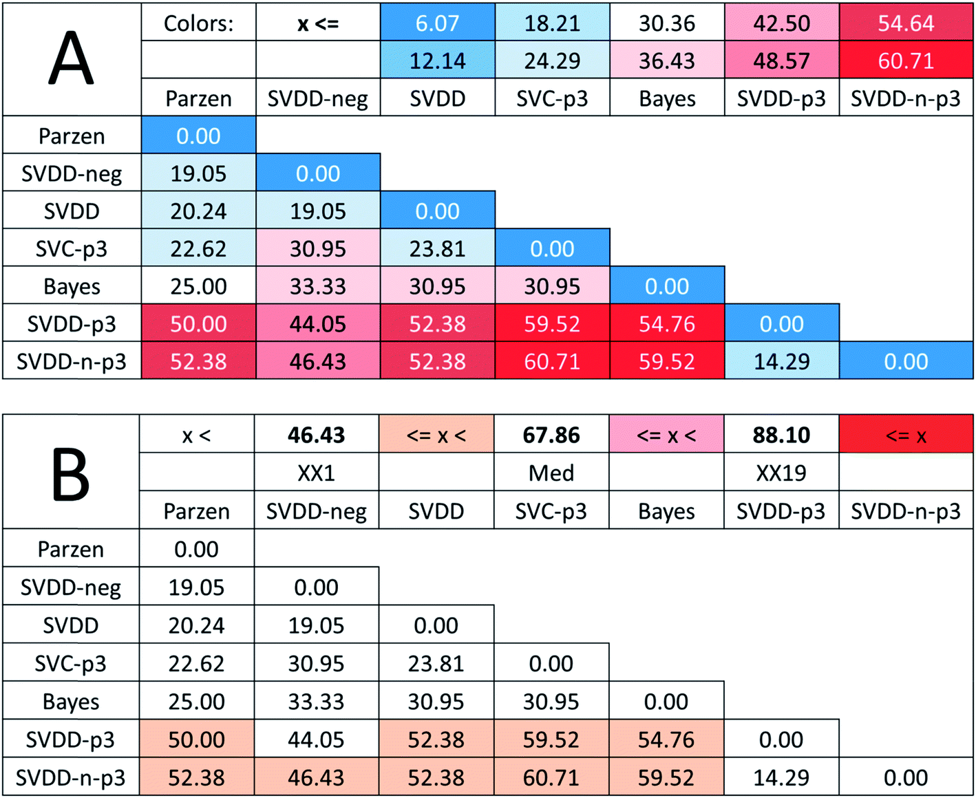 | ||
| Fig. 7 Heatmap representations of SRD-COVAT matrices for Case study 2. (A) SRD values increase in the blue (highest similarity) towards red (lowest similarity) direction. The classifiers are enumerated in the order of increasing sums of SRD values. (B) The same table with a different coloring scheme highlights those pairs of methods that are the most discordant. If the given SRD value overlaps with the frequency distribution of random ranking, other colors than white were applied. Thus, if one of the methods of such a pair is used as reference, the other one is not significantly more similar to it than the use of random numbers, in terms of ranking. For both tables, color codes are provided in the header with relative (%) values. | ||
GPCM (conditional exact Fisher's test and probability-weighted ordering) provides the same pattern: Parzen and Min provide identical (always zero) values (see Table 2 in ESI†). The last three items cannot be distinguished from random ranking. GPCM clearly differentiates three clusters among these methods: I (Parzen, identical with Best (Min), II (SVDD-neg, SVDD, SVC-p3, Bayes) and III (SVDD-n-p3, SVDD-p3, Max)). Knowing that the background philosophy and calculations of GPCM and SRD are entirely different, the concordance of the rankings is noteworthy.
3.3 Case study 3
González Martín et al. evaluated electronic nose results of vegetable oils with various classification methods.23 The percentages of correct classifications and predictions of KNN, LDA, QDA, and SIMCA were compared (the detailed results are listed in their Tables 1, 3, 4 and 5). Following their work, we have also included the methods when used with raw data (denoted with r, for example, SIMCAr), as well as normalized data (denoted with n, for example, SIMCAn). In addition, LDA was included when using all available variables (48), and a smaller subset after variable selection (5). The authors concluded that SIMCA and KNN have the worst performance, while LDA showed the best one.SRD was used to create a more detailed comparison and a clear ranking. This ranking was in accordance with the authors' conclusions. Fig. 8 shows that SIMCA has a slightly better performance than KNN, which is positioned after the 5% probability level. On the other hand, the best performances were observed for QDA and LDA. In the case of LDA, using more variables gave better performance. Normalization, on the other hand, decreased the performance of LDA (in contrast with the other methods).
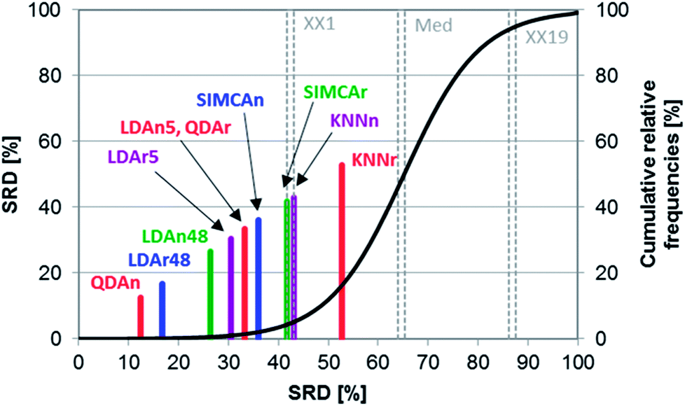 | ||
| Fig. 8 SRD result of Case study 3. Normalized SRD values (percentages) are plotted on the x and left y-axes. Cumulative relative frequencies (also in percentages) are on the right y-axis. The latter is fitted with a hyperbolic tangent function (cumulative probabilities of a fitted Gauss curve). | ||
Leave-one-out cross-validation was used as a validation process for the SRD values. The result of the validation is summarized on a box and whisker plot, see Fig. 9. The cross-validated result was used for significance testing as well. Thus, nonparametric sign and Wilcoxon tests were used for this purpose. The results showed that the LDAn5, QDAr and SIMCAn methods are not significantly different from each other (at α = 0.05 level).
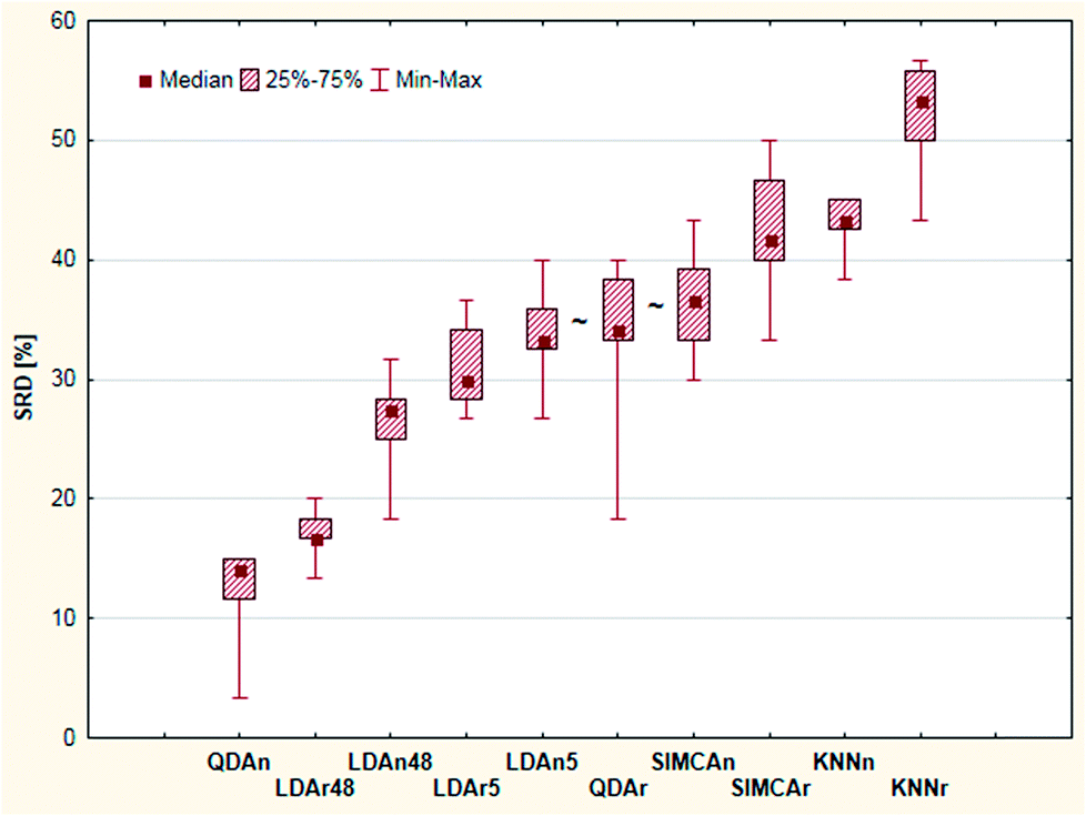 | ||
| Fig. 9 Box and whisker plot of Case study 3. Cross-validated SRD values (%) are plotted on the y-axis. The non-significantly different methods are marked with the “∼” symbol. | ||
From the SRD-COVAT results (Fig. 10), it is noteworthy that many of the studied methods are significantly discordant with each other (their SRD values overlap with random ranking many times). In particular, this is even the case for two pairs of LDA methods (LDAr5 and LDAn48, and LDAn5 and LDAr48).
 | ||
| Fig. 10 Heatmap representation of the SRD-COVAT matrix for Case study 3. If the given SRD value overlaps with the frequency distribution of random ranking, other colors than white were applied. Thus, if one of the methods of such a pair is used as reference, the other one is not significantly more similar to it than the use of random numbers, in terms of ranking. Color codes are provided in the header with relative (%) values. | ||
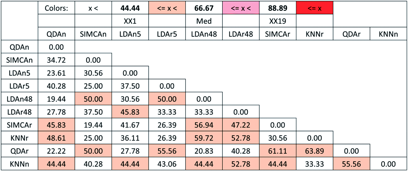
GPCM (conditional exact Fisher's test and probability-weighted ordering) provides the same pattern: QDAn, LDAr48, LDAn48, and LDAr5 are placed on the first four ranks. The GPCM results can be seen in Table 4 in ESI.†
GPCM clearly differentiates six clusters among these methods: I (QDAn), II (LDAr48), III (LDAn48 and LDAr5), IV (QDAr, LDAn5, SIMCAn), V (KNNn) and VI (SIMCAr, KNNr). Again, GPCM and SRD show similar results while they are based on completely different calculations.
3.4 Case study 4
In the remarkable work of Forina et al. several classic and novel class-modeling techniques were compared and discussed based on real datasets.6 Artificial datasets were also used for the explanation of the methods. Sensitivity, specificity (proportion of observed negatives that were predicted to be negatives), and efficiency (the mean of sensitivity and specificity) of the applied models played an important role in their comparison. SIMCA, UNEQ, univariate range modeling (URM) and multivariate range modeling (MRM) methods were used for classification.In this case study, we have compared the above mentioned class-modeling techniques based on their performances on real datasets (wines, olive oil, etc.). The following performance parameters were used for the analysis: (a) mean of sensitivity (cross-validation), (b) mean of specificity (cross-validation), (c) efficiency (cross-validation), and (d) specificity in the case of 100% sensitivity (final model). Efficiency was calculated as the average of sensitivity and specificity. SIMCA was discussed earlier in details and UNEQ is also a frequently used technique, but here the different variances of the groups have not caused any difficulties. URM and MRM are more recent and related techniques. While URM is based on the allowed range of the exact original variables, MRM applies principal components or discriminant variables (like the canonical variables of LDA). The authors of the original paper correctly stated that URM is a method with weaker performance than MRM.
The performance values of four real datasets were used for the SRD and GPCM analyses. The final merged data matrix contained 16 rows (performance parameters) and four columns (methods). Row maxima were used as reference in both cases. The final result can be seen in Fig. 11. It clearly shows that the best and most consistent method was MRM based on these data, while the other three techniques gave almost the same results.
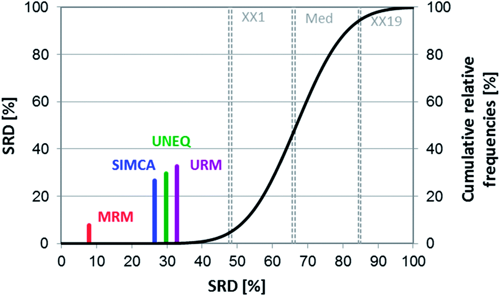 | ||
| Fig. 11 SRD results of Case study 4. Normalized SRD values (percentages) are plotted on the x and left y-axis, and cumulative relative frequencies (also in percentages) are on the right y-axis. The latter is fitted with a hyperbolic tangent function (cumulative probabilities of a fitted Gauss curve). | ||
Cross-validation also helps to decide whether the ranking behavior of these methods is significantly different from each other. Sevenfold cross-validation was used to validate the SRD results. For this purpose, a box and whisker plot was made for the cross-validated SRD values (Fig. 12). On the other hand, nonparametric sign tests and Wilcoxon matched pair statistics were also calculated. The final results showed in every case that the SIMCA, UNEQ and URM techniques are not significantly different.
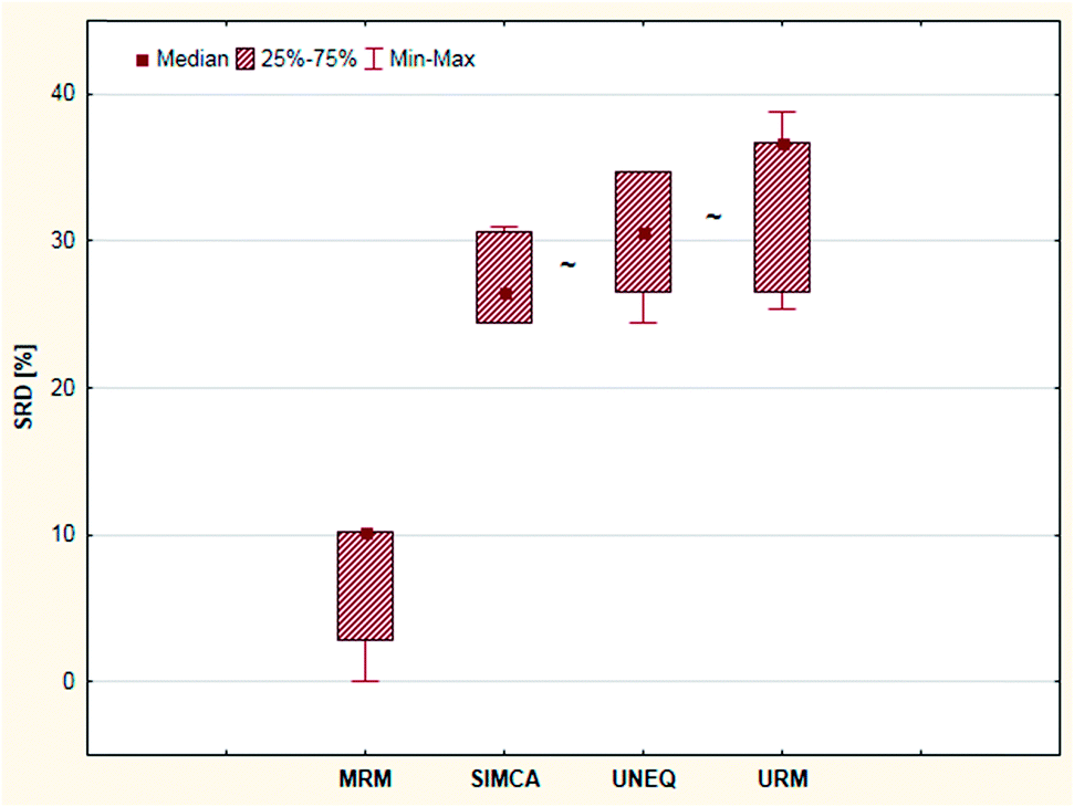 | ||
| Fig. 12 Box and whisker plot of Case study 4. Cross-validated SRD values (%) are plotted on the y-axis. The non-significantly different methods are marked with the “∼” symbol. | ||
GPCM analysis gave results in agreement with the SRD calculations (Table 5, ESI†). Conditional exact Fisher's test and probability-weighted ordering were used for the analysis. Here, the MRM method was also the best, while the other three methods are virtually indistinguishable.
MRM was clearly the best and most consistent method for classification in this case. Although the other three techniques – including SIMCA – were better than the use of random numbers (based on SRD), the results of these methods were less promising and indistinguishable from each other in the statistical sense. This conclusion is in harmony with the statement of the authors of the original article: “it seems possible to conclude that MRM is a technique with excellent performances…”.6
3.5 Case study 5
Shaffer et al. compared several pattern recognition algorithms (neural network, nearest neighbor and linear discriminant analysis based ones) on chemical sensor array datasets.24 Probabilistic neural networks (PNN), learning vector quantization (LVQ) neural networks, back-propagation artificial neural networks (BP-ANN), soft independent modeling of class analogies (SIMCA), Bayesian linear discriminant analysis (BLDA), Mahalanobis linear discriminant analysis (MLDA) and the nearest-neighbor (NN) methods were compared based on the classification accuracy of the models. LVQ can be explained as the combination of NN and competitive learning ANNs. The techniques are briefly introduced in the original paper. Four datasets were used, two simulated and two real. Although the authors compared the methods based on their speed, training difficulty, memory requirements, etc. as well, we have complemented the comparison, using the classification accuracies (correct classification rates) for each dataset.The aforementioned classification accuracy data was used for the SRD and GPCM analysis. In both cases, maximum classification accuracy was applied as the golden reference. The data matrix contained eight rows (datasets – training and test sets) and seven columns (pattern recognition methods) for the calculation procedures. Leave-one-out cross-validation was used for SRD calculations. Results of SRD are presented in Fig. 13 and 14 (cross-validated results). It is clear that the best method was BP-ANN, and MLDA gave the worst result.
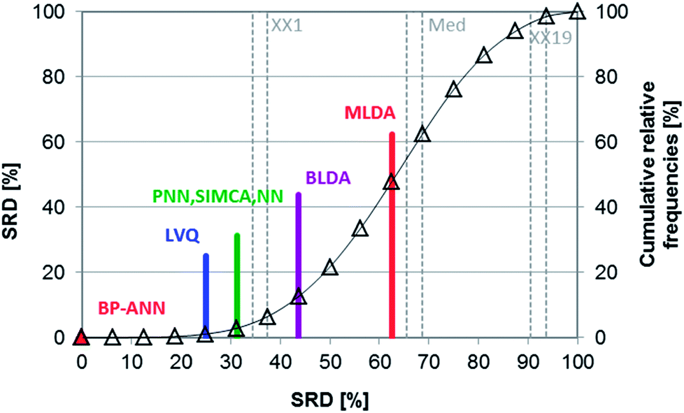 | ||
| Fig. 13 SRD results of Case study 5. Normalized SRD values (percentages) are plotted on the x and left y-axis, and cumulative relative frequencies (also in percentages) are on the right y-axis. The latter is fitted with a hyperbolic tangent function (cumulative probabilities of a fitted Gauss curve). | ||
 | ||
| Fig. 14 Box and whisker plot of Case study 5. Cross-validated SRD values (%) are plotted on the y-axis. The non-significantly different methods are marked with the “∼” symbol. | ||
Nonparametric sign tests and Wilcoxon tests, as well as Student's t-tests, were calculated for the cross-validated SRD values to decide whether the methods are significantly different. The results showed that NN, PNN, and SIMCA are equivalent in the statistical sense.
GPCM results are only slightly different from SRD ranking (Table 6, ESI†). Conditional exact Fisher's test and probability-weighted ordering were used for the analysis. The results clearly confirm the SRD ranking, because BP-ANN is the best and the NN, PNN, LVQ techniques have a slight difference in the probability values.
However, the authors stated that “Both PNN and LVQ require fewer adjustable parameters than BP-ANN, which results in faster training times and implies a more reliable classifier”. On the other hand, our statement is that all neural network based methods, especially BP-ANN can easily be overoptimized, while the features of LVQ are not fully back-traceable, moreover, it can be a more appropriate method for the classification problems than BP-ANN in the sense of classification accuracy. A great advantage of the proposed approach is that SRD and GPCM are able to rank biased estimations as well, because the biases of various methods follow normal distribution, similarly to random errors.
3.6 Case study 6
The following case study is based on a comparative study by Tominaga on classification techniques with the use of three types of chemotherapeutic agents: antibacterials, antineoplastics, and antifungals.25 The applied compounds are registered in the MDL drug data report (MDDR) database. The classification models were made with principal component analysis – linear discriminant analysis (PCA-LDA), soft independent modeling of class analogies (SIMCA), partial least squares 2 (PLS2), artificial neural networks (ANN), the nearest neighbor method (NN), the combination of NN with Ward clustering (W-NN) and a genetic algorithm (GA-NN). Training and test sets were used separately and the test set samples were registered in the comprehensive medicinal chemistry (CMC) database. In the case of PLS2, three different dependent variables were used for the prediction.SRD and GPCM methods were used similarly as in the case studies mentioned above. The applied dataset contained the percentage of the correctly predicted samples (correct classification rate for prediction). Maximum was used as reference, and leave-one-out cross-validation was used for validation. SRD results are presented in Fig. 15 (cross-validated).
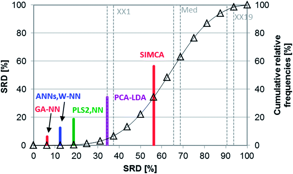 | ||
| Fig. 15 SRD results of Case study 6. Normalized SRD values (percentages) are plotted on the x and left y-axes, and cumulative relative frequencies (also in percentages) are on the right y-axis. The latter is fitted with a hyperbolic tangent function (cumulative probabilities of a fitted Gauss curve). | ||
According to Fig. 15, the most consistent method was GA-NN and without doubt, SIMCA gave the worst result in this case study. Knowing the easily overfitted character of the neural network based methods, it cannot be surprising that genetic algorithm or Ward clustering combined with nearest neighbors gives better results than the ANN. However, this was hidden information in the original dataset.
Nonparametric tests (sign tests and Wilcoxon matched pair tests) were also used here to decide whether the methods are significantly different. The final result showed that there is no significant difference between the results of the ANN, W-NN, NN and PLS2 methods (Fig. 16). GPCM was carried out in the same manner as in the previous cases; the results are presented in ESI Table 7.† This result is slightly different from SRD ordering, but the most consistent four methods are the same. SIMCA was the worst method in both cases.
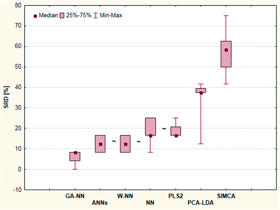 | ||
| Fig. 16 Box and whisker plot of Case study 6. Cross-validated SRD values (%) are plotted on the y-axis. The non-significantly different methods are marked with the “∼” symbol. | ||
4. Discussion
The presented meta-analysis evaluated six, carefully selected case studies from the literature. A common characteristic of these case studies is that their data structure is different but the same classification task was carried out. One of the advantages of our presented approach is the general applicability and general conclusions drawn based on all data sets, which can be later used by researchers.The findings of our work are supported by many other sources, for example, similar conclusions were communicated by Mazzatorta et al. in 2004.26 The authors have compared seven classification algorithms for toxicity prediction on a dataset of 235 pesticides and 153 descriptors and have concluded their work by recommending primarily regularized discriminant analysis and classification and regression trees. While they have evaluated soft independent modeling of class analogies (SIMCA) generally positively, they note that its big disadvantage is its sensitivity to data scaling. Also, their Table 2 lists SIMCA as the worst performing method in many cases and it is also apparent that its performance (as expressed by non-error rates) differs significantly during fitting and cross-validation.
In a study on pharmaceutical excipients, Candolfi et al. have applied near-infrared spectroscopy with SIMCA and concluded (among others) that about 15% of the samples are rejected from their own classes (α-error). This can be connected to the heterogeneous nature of the NIR spectra from different batches and suppliers or the small number of training objects, but the influence of the properties and parameters of SIMCA – such as its parametric character or the number of latent variables used – cannot be overlooked either. Pre-processing of the spectra did not influence the results in this study, but it can be useful in general to remove spectral information of physical rather than chemical origin (e.g. information related to particle size) and to increase between-class variance.27
Frank and Lanteri compared classification models using four data sets, selected from various fields of chemistry. LDA, QDA, SIMCA and classification and regression trees (CART) were used and although the authors did not state, which one is the absolute winner, the percentage of correctly classified observations shows that SIMCA has more misclassifications compared to CART. The authors state, however, that from the viewpoint of complexity and interpretability, CART is the best choice because it uses a few terminal nodes (a node of a tree data structure that has no child nodes) and the unknown samples can be classified manually.28
Mid-infrared spectroscopy (MIR) and near-infrared spectroscopy (NIR) were used to evaluate crude petroleum oils and virgin olive oils by Galtier et al. The authors applied several chemometric methods: SIMCA, partial least squares regression discriminant analysis (PLS2-DA), PLS2-DA with SIMCA, and PLS1-DA in two infrared spectroscopic applications. Their aim was to compare the methods based on their classification results after optimization on the basis of spectral variance analysis. Although for petroleum oils, all the methods gave 100% correct classification percentage (CC%), their results were not so convincing for virgin olive oils. The CC% clearly shows that SIMCA is always inferior compared to the other methods in different spectral ranges; hence the authors conclude that PLS-DA outperforms SIMCA.29
SIMCA also showed a relatively poor performance when compared to Kohonen artificial neural networks (Kohonen) and unequal dispersed classes (UNEQ). Marini et al. presented a class-modeling technique based on Kohonen artificial neural networks and compared its classification performance to SIMCA and UNEQ. Eight physical and technological determinations on 1779 Italian samples of rice from 11 varieties have been used for the data analysis, Kohonen, UNEQ, and SIMCA scored 91.30%, 89.31% and 88.53% CC%, respectively.30
An interesting drawback of SIMCA has been shown by Nejadgholi and Bolic, who compared PCA, SIMCA and the ‘Cole model’ for classification of bioimpedance spectroscopy (BIS) measurements. The authors showed that while SIMCA achieved 100% CC on the training datasets, its results dramatically dropped (22%) after leave-one-out cross-validation (LOOCV). However, PCA combined with KNN showed lower CC% on the training data (97%) but had good LOOCV results (90%).31
Moreda-Piñeiro et al. have compared the performance of LDA and SIMCA on a dataset of Asian and African tea samples (concentration of 17 elements determined with ICP-AES and ICP-MS), for classification based on geographical origin.32 The performance of SIMCA was found to be inferior to LDA in two different tasks: the classification of African vs. Asian tea samples, and the classification of Chinese, Indian and Sri Lankan samples. It is worth to note that in the latter case, PCA-based separation of Indian and Sri Lankan samples was not possible, either. However, LDA could classify these samples with a 100% correct classification rate nonetheless (here, CC% values of SIMCA for these two groups were around 30%).
Flood et al. have compared KNN, PLS, and SIMCA for classification of Diesel fuel types. Considering SIMCA, their experience is unambiguous: “KNN proves to be a powerful method of prediction for both concentration and feedstock, while SIMCA was more challenged for classification of the multifeedstock blends.”33
A drawback of SIMCA (and possibly the reason of its poorer performance in comparison to other classification methods) is that “the class subspaces are built independently […], the discriminative between-class information is neglected”.34 To overcome this problem, the original data can be projected to a more discriminative subspace (prior to classification with SIMCA). In a recent work, Zhu et al. have introduced discriminatively ordered subspace (DOS) for this purpose and compared it to an existing subspace projection method (generalized difference subspace or GDS), as well as SIMCA (without subspace projection) and LDA (as an independent benchmark method).34 Based on a comparison on three real datasets, the authors conclude that DOS projection can increase the performance of SIMCA to a greater extent than GDS (in fact, GDS deteriorates the classification accuracies in two of the three cases). While there is a noticeable improvement in the classification accuracies when applying DOS projection (as compared to SIMCA without projection), it is unclear from the published box and whisker plot, whether these differences are statistically significant or not. Nonetheless, the authors propose further ideas for improved subspace projection methods.
Another example of SIMCA discrimination can be found in ref. 35 Statistical models were constructed for the characterization of the botanical and geographical origin. The performance of LDA and SIMCA was compared and the models were validated with a randomized batchwise procedure. SIMCA performance is downgraded between 3–17% and 2–13% in correct classification for Tables 2 and 3 respectively.
5. Conclusions
In this work, we provide a general framework for comparison of various classifiers: two non-parametric methods, sum of ranking differences (SRD) and the generalized pairwise correlation methods (GPCM), have provided highly similar ranking and grouping of the classification techniques, although they are based on entirely different principles. The ordering by SRD was validated with a randomization test and cross-validation. Whereas SIMCA frequently (but not always) passed the randomization test, cross-validation unambiguously proves its inferiority to other techniques in supervised classification tasks.While SRD and GPCM are sensitive to the reference selection (supervisor), this effect could be eliminated with comparisons with one classifier at a time (SRD-COVAT) and the resulting heatmaps support and validate the grouping pattern found by using the above two techniques. Considering highly different and deviating data sets, soft independent modeling of class analogies (SIMCA) has proven to be of weak performance (worst among the studied methods in numerous cases), despite its advantages and unique theoretical background. SIMCA has never appeared as the best method in any examined comparison here, out of a total of 29 methods in the six case studies. (Due to the different names used by the different authors, there is some overlap among the 29 methods, but they encompass most of the major branches of classification methods: artificial neural networks, linear and quadratic discriminant analyses, CAIMAN, Support vector classifier, PLS-DA, K-nearest-neighbor, Bayesian and Parzen classifiers, CART, learning vector quantization, nearest mean classifier, UNEQ, uni- and multivariate range modeling.) There is no doubt that circumstances can be found, when SIMCA is superior to other techniques, but these are not typical situations.
SIMCA was created primarily as a class-modeling method, and although it can be used as a discriminant tool, this is not the primary aim of the method. However, the vast majority of SIMCA usage is for classification and not class modeling. When using SIMCA as a discriminant tool, its performance is inferior to the compared methods. Naturally, these results do not suggest that SIMCA should be avoided, but in light of the presented results, the present authors would reserve its use for cases where the possibility of assigning samples into more classes or no class at all (i.e. “class modeling” or “soft modeling”) is truly of importance. SIMCA might provide good results in “one class” situations, which can be used for determination of authenticity for samples. However, no such method comparison can be provided, as other classifiers require at least two classes. If we consider the “not-in-class” samples as another class, the case simplifies to a binary classification where SIMCA shows weak performance. Nevertheless, our results emphasize the importance of model (and method) comparison, which can be easily done using the above proposed methodology. Our results, along with several other studies clearly suggest that usually better options than SIMCA exist for the same (real or simulated) datasets for supervised pattern recognition. Alternatively, the performance of SIMCA can be enhanced with subspace projection methods, although this area still has a long way to go.
It should be noted, that a classification method cannot always be superior to others, since performances depend on the classification task and conditions. However, a hypothetical best method can be defined, which provides the maximal performance (maximal correct classification rate) on the given dataset. Sum of ranking differences is capable of comparing classification methods to this hypothetical best one; hence providing a reliable, validated approach for method selection.
Conflicts of interest
There are no conflicts of interest to declare.Acknowledgements
The authors thank the support of the National Research, Development and Innovation Office of Hungary (OTKA, contracts No. K119269 and KH-17 125608).References
- L. A. Berrueta, R. M. Alonso-Salces and K. Héberger, J. Chromatogr. A, 2007, 1158, 196–214 CrossRef CAS PubMed.
- S. Wold and M. Sjöström, in Chemometrics Theory and Application, ed. B. R. Kowalski, American Chemical Society, 1977, pp. 243–282 Search PubMed.
- K. Vanden Branden and M. Hubert, Chemom. Intell. Lab. Syst., 2005, 79, 10–21 CrossRef CAS.
- G. R. Flåten, B. Grung and O. M. Kvalheim, Chemom. Intell. Lab. Syst., 2004, 72, 101–109 CrossRef.
- L. Mannina, F. Marini, M. Gobbino, A. P. Sobolev and D. Capitani, Talanta, 2010, 80, 2141–2148 CrossRef CAS PubMed.
- M. Forina, P. Oliveri, S. Lanteri and M. Casale, Chemom. Intell. Lab. Syst., 2008, 93, 132–148 CrossRef CAS.
- B. K. Lavine and W. S. Rayens, in Comprehensive Chemometrics, 2009, pp. 507–515 Search PubMed.
- K. Héberger and K. Kollár-Hunek, J. Chemom., 2011, 25, 151–158 CrossRef.
- K. Héberger, TrAC, Trends Anal. Chem., 2010, 29, 101–109 CrossRef.
- D. Bajusz, A. Rácz and K. Héberger, J. Cheminf., 2015, 7, 20 Search PubMed.
- A. Rácz, D. Bajusz and K. Héberger, SAR QSAR Environ. Res., 2015, 26, 683–700 CrossRef PubMed.
- W. J. Conover, in Practical Nonparametric Statistics, Wiley, 3rd edn, 1999, pp. 157–176 Search PubMed.
- F. Wilcoxon, Biom. Bull., 1945, 1, 80–83 CrossRef.
- F. Andrić, D. Bajusz, A. Rácz, S. Šegan and K. Héberger, J. Pharm. Biomed. Anal., 2016, 127, 81–93 CrossRef PubMed.
- J. H. Kalivas, B. Brownfield and B. J. Karki, J. Chemom., 2017, e2873 CrossRef.
- A. J. Tencate, J. H. Kalivas and A. J. White, Anal. Chim. Acta, 2016, 921, 28–37 CrossRef CAS PubMed.
- J. H. Kalivas and J. Palmer, J. Chemom., 2014, 28, 347–357 CrossRef CAS.
- K. Héberger and R. Rajkó, J. Chemom., 2002, 16, 436–443 CrossRef.
- R. Todeschini, D. Ballabio, V. Consonni, A. Mauri and M. Pavan, Chemom. Intell. Lab. Syst., 2007, 87, 3–17 CrossRef CAS.
- B. G. M. Vandeginste, D. L. Massart, L. M. C. Buydens, S. De Jong, P. J. Lewi and J. Smeyers-Verbeke, in Handbook of Chemometrics and Qualimetrics, Part B, Elsevier B.V., Amsterdam, Netherlands, 1998, pp. 207–241 Search PubMed.
- Using Cross-Validation, http://wiki.eigenvector.com/index.php?title=Using_Cross-Validation, July 11, 2017.
- D. M. J. Tax, One-class classification. Concept-learning in the absence of counter-examples, Proefschrift, Ph.D.thesis, Technische Universiteit Delft, 2001.
- Y. González Martín, M. C. Cerrato Oliveros, J. L. Pérez Pavón, C. García Pinto and B. Moreno Cordero, Anal. Chim. Acta, 2001, 449, 69–80 CrossRef.
- R. E. Shaffer, S. L. Rose-Pehrsson and R. A. McGill, Anal. Chim. Acta, 1999, 384, 305–317 CrossRef CAS.
- Y. Tominaga, Chemom. Intell. Lab. Syst., 1999, 49, 105–115 CrossRef CAS.
- P. Mazzatorta, E. Benfenati, P. Lorenzini and M. Vighi, J. Chem. Inf. Model., 2004, 44, 105–112 CrossRef CAS PubMed.
- A. Candolfi, R. De Maesschalck, D. Massart, P. Hailey and A. C. Harrington, J. Pharm. Biomed. Anal., 1999, 19, 923–935 CrossRef CAS PubMed.
- I. E. Frank and S. Lanteri, Chemom. Intell. Lab. Syst., 1989, 5, 247–256 CrossRef CAS.
- O. Galtier, O. Abbas, Y. Le Dréau, C. Rebufa, J. Kister, J. Artaud and N. Dupuy, Vib. Spectrosc., 2011, 55, 132–140 CrossRef CAS.
- F. Marini, J. Zupan and A. L. Magrì, Anal. Chim. Acta, 2005, 544, 306–314 CrossRef CAS.
- I. Nejadgholi and M. Bolic, Comput. Biol. Med., 2015, 63, 42–51 CrossRef PubMed.
- A. Moreda-Piñeiro, A. Fisher and S. J. Hill, J. Food Compos. Anal., 2003, 16, 195–211 CrossRef.
- M. E. Flood, M. P. Connolly, M. C. Comiskey and A. M. Hupp, Fuel, 2016, 186, 58–67 CrossRef CAS.
- R. Zhu, K. Fukui and J.-H. Xue, Inf. Sci., 2017, 382, 1–14 CrossRef.
- T. Nietner, M. Pfister, M. A. Glomb and C. Fauhl-Hassek, J. Agric. Food Chem., 2013, 61, 7225–7233 CrossRef CAS PubMed.
Footnote |
| † Electronic supplementary information (ESI) available. See DOI: 10.1039/c7ra08901e |
| This journal is © The Royal Society of Chemistry 2018 |