DOI:
10.1039/C8QM00162F
(Research Article)
Mater. Chem. Front., 2018,
2, 1674-1691
Introduction of newly synthesized Schiff base molecules as efficient corrosion inhibitors for mild steel in 1 M HCl medium: an experimental, density functional theory and molecular dynamics simulation study†
Received
10th April 2018
, Accepted 2nd July 2018
First published on 5th July 2018
Abstract
The purposeful incorporation of aliphatic, branched chain and substituted aromatic moieties in the molecular skeleton of organic Schiff bases, in line with corrosion inhibition performance, has been conducted. Three Schiff bases, namely, 2-((2-hydroxyethylimino)methyl)-6-methoxyphenol (L1), 2-((1-hydroxybutan-2-ylimino)methyl)-6-methoxyphenol (L2) and 2-(2-hydroxy-3-methoxybenzylideneamino)phenol (L3) were synthesized and subsequently assessed for the inhibition of mild steel corrosion in 1 M HCl medium. The corrosion inhibition proficiencies of the synthesized inhibitors on the mild steel surface have been investigated by gravimetric measurements, electrochemical analysis (potentiodynamic polarization, electrochemical impedance spectroscopy), surface morphological studies (FESEM and AFM), contact angle measurement and, most importantly, theoretical studies. The results obtained from the gravimetric as well as electrochemical measurements revealed that the studied Schiff bases are mixed-type inhibitors that show maximum inhibition efficiency up to ∼97% at the concentration of 5 mM. In theoretical studies, atomic-level calculations give deeper insights into the corrosion inhibition mechanism and the relative performance of present inhibitors. However, it has been found that normal density functional theory (DFT) calculations are not sufficient to deal with the interactions between inhibitors and metal surfaces in complex systems. As such, in order to investigate inhibitor–metal interactions, herein, the density functional tight binding (DFTB) approach has been introduced as formulated by Hohenberg, Kohn and Sham (KS-DFT). Furthermore, for more insightful studies, e.g., growth characteristics, as well as the selection of a more stable surface of the α-Fe crystal morphology studies, have also been performed using the “morphology” module. The morphology of the α-Fe crystal in equilibrium was analyzed using the Wulff construction plot. In DFTB calculations, the trans3d Slater–Koster library set has been implemented for possible pairs of interactions between inhibitor–metal complex systems (C, N, O, H and Fe). Some salient features like equilibrium adsorption configuration and charge density difference obtained from DFTB calculations have been described in detail. Furthermore, for comparison with the real world of corrosion inhibition, molecular dynamics (MD) simulation was employed in the presence of all concerned species (inhibitor molecule, Fe surface, H2O, H3O+ and Cl−), which revealed the actual adsorption configurations of the inhibitor molecule on the desired metallic surfaces.
Metallic corrosion has become one of the major safety and economic concerns in almost all industries all over the world. Metals and their alloys undergo chemical or electrochemical reactions with the environment and get severely corroded. Among the several metals, the most profusely exploited material for construction purposes is mild steel, owing to its excellent mechanical properties and comparatively low cost compared to other materials.1,2 It is mostly used in large amounts in chemical processing, marine applications, metal processing equipment and refining construction related works in petroleum production units.3 However, in several industrial applications, hydrochloric acid, sulphuric acid and nitric acid are extensively employed for numerous techniques, such as acid cleaning, acid descaling, pickling of metals, acidizing of oil wells, recovering ion exchangers, etc.3–7 Unfortunately, as a result, mild steel has faced serious metallic corrosion in the aggressive acidic solutions and thereby huge economic losses are incurred worldwide. Among the several available corrosion inhibition techniques to restrict the acid-induced metal degradation, the use of organic molecules as inhibitors have emerged as a vibrant field of research.8–11 The incorporation of heteroatoms (e.g. N, O, S, P), unsaturated π-bonds, planar and conjugated aromatic rings allow organic inhibitors to be adsorbed onto the metallic surfaces and thereby prevent further acidic attack.12–18
Nowadays, among the several classes of organic inhibitors, Schiff bases have gained enormous attention as anticorrosion materials due to their straightforward synthesis procedure, high purity, cost-effective starting precursors, low toxicity and most importantly their environmentally friendly nature.19–23 In the recent past, structurally almost similar compounds (as reported here) have been used as chemosensors where the in vitro detection of picric acid has been carried out using fluorescence microscopy. In this process, it has been noticed that the compound can penetrate the cell membrane without causing any impairment.24a In another study, it has also been found that similar Schiff base ligands (as reported here) have antibacterial and anticancer properties.24b This reflects their environmentally friendly and non-toxic nature.
In addition to the environmentally friendly nature, the choice of inhibitor molecules is also based on their structural considerations. Herein, to analyze the adsorption behaviour of aliphatic chain and aromatic moieties, initially, the aromatic moiety is coupled with a small aliphatic chain by a simple azomethine linkage and thereafter, the aliphatic chain is extended to some extent and is ultimately further extended up to the cyclization of the aromatic ring. Here, the intention is to see how their stereochemical configurations affect their adsorption capabilities, which in turn influence their corrosion inhibition ability.
In view of this, the present investigation has been carried out by synthesizing three Schiff bases, namely, 2-((2-hydroxyethylimino)methyl)-6-methoxyphenol (L1), 2-((1-hydroxybutan-2-ylimino)methyl)-6-methoxyphenol (L2), 2-(2-hydroxy-3-methoxybenzylideneamino)phenol (L3) as anticorrosion materials and their corrosion inhibiting efficiencies were investigated on mild steel in 1 M HCl medium. To the best of our knowledge, this is the first time that these molecules are being explored as inhibitors for mild steel corrosion inhibition in 1 M HCl medium.
The corrosion inhibition performance of the synthesized inhibitor molecules was carried out by electrochemical techniques such as electrochemical impedance spectroscopy (EIS) and potentiodynamic polarization measurements. From these techniques, the inhibition efficiency of the aforementioned inhibitor molecules is easily analyzed. However, these techniques cannot explore the actual inhibition mechanism on the metal solution interface. It is also unable to explain why small modifications in the molecular skeleton of the inhibitor molecules impose a profound effect on their inhibition efficiencies. On this occasion, we focused our attention on computer-assisted simulation techniques. Due to the development of efficient hardware and software in the computer related system, it is highly possible to provide an explanation regarding the inhibitive performances of inhibitors from the atomic as well as the molecular level of theory.25–27 From the literature, it was also found that among the several available theoretical techniques, density functional theory (DFT) and molecular dynamics (MD) simulation are the most authentic in order to establish the relationship between the molecular properties of the inhibitors and their corresponding inhibition efficiencies.4,7,12–16 In recent times, proper implementation of such theoretical approaches have simultaneously predicted and accurately explored the corrosion inhibitive performance of aminobenzonitrile derivatives,15 pyrazine derivatives,25 benzimidazole derivatives16 and Schiff base molecules12–14 from their atomistic and molecular levels of investigation. However, it is obvious that normal DFT cannot deal with the real environment of corrosion inhibition. In normal DFT, only the molecular properties of the inhibitors in the solution phase are considered; however, how a molecule behaves in an actual situation, is very difficult to properly define with the normal DFT calculations. From this perspective, this is probably the first time in corrosion inhibition chemistry that we have introduced the density functional tight binding (DFTB) method for the possible pairing of interactions between the inhibitor and the metal surfaces. DFTB is a quantum mechanical method that is derived from DFT via several approximations.28 This method has been particularly designed for the complex molecular systems. DFTB is a parameterized method and its accuracy may depend extensively on the quality of the parameterization. In particular, it requires the use of parameterized integrals, generally referred to as the Slater–Koster integrals, constructed for each atom pair of the chemical system of interest. In the particular case of inhibitor–metal interactions, the trans3d Slater–Koster library set is used for the possible pairing of interactions between the C, N, O, H and Fe. Overall, DFT, DFTB and most importantly MD simulation give more fruitful results towards the development of better and effective organic corrosion inhibitor molecules.
In the present investigation, we intend to analyze how the stereochemical configuration and molecular properties of inhibitor molecules influence the corrosion inhibitive properties of the molecules. To do this, first of all, the corrosion inhibiting performance of Schiff base compounds in 1 M HCl medium have been investigated by gravimetric analysis, potentiodynamic polarization and electrochemical impedance spectroscopy (EIS) techniques. Furthermore, the morphology of corroded metal surfaces without and with the application of inhibitor molecules has been analyzed by the field emission scanning electron microscopy (FESEM) and atomic force microscopy (AFM). The extent of the hydrophilic or hydrophobic properties of the protective layer formed on the surface of mild steel has been analyzed by the contact angle measurement. In general, normal DFT has been performed to analyze how molecular arrangement in space and molecular properties of the inhibitor molecules influence the corrosion inhibition properties of the inhibitors. Afterwards, the DFTB method was implemented for the possible mode of interaction between the inhibitor molecule and Fe surface atoms. Equilibrium adsorption configuration and charge density differences for the adsorption systems obtained from DFTB calculation have been investigated in detail. In addition, to mimic a real corrosion environment, the MD simulation was carried out in the presence of all concerned species that actually take part in corrosion.
Experimental details
Materials
Analytical grade chemicals and solvents were used for synthesis purposes. 2-Hydroxy-3-methoxybenzaldehyde, 2-aminoethanol, 2-aminobutan-1-ol and 2-aminophenol were procured from Alfa Aesar and used without further purification. From Merck India, GR grade HCl (35%) was obtained. Methanol, acetone and ether were purchased from Fluka and used without further purification.
Instrumentation
In order to collect the microanalytical (C, H, N) data, a Perkin Elmer 2400C elemental analyzer was used. FT-IR studies were carried out using a Perkin Elmer FT-IR spectrometer (spectrometer 100). The mass spectra were recorded using an Advion compact mass spectrometer (serial no. 3013-0140). 1H and 13C NMR experiments were carried out on Bruker 300 MHz NMR spectrometer. A Biologic, France SP-150 Potentiostat/Galvanostat Instrument was used to perform all the electrochemical experiments. Surface morphology studies of the mild steel samples were investigated using a Σigma HD, Zeiss, Germany. AFM analysis was carried out using a Nanosurf, C3000 instrument. Contact angle measurements were performed using an OCA 15pro commercial goniometer (Dataphysics, Germany).
Synthesis of inhibitor molecules
Three Schiff base molecules were synthesized by a simple condensation reaction between equimolar amounts of 2-hydroxy-3-methoxybenzaldehyde and corresponding amines (2-aminoethanol, 2-aminobutan-1-ol and 2-aminophenol) in the methanolic medium. The excess solvent was evaporated using a rotary evaporator and the obtained product was washed several times with ether and finally dried in air. The compounds were characterized by elemental analysis, FTIR, ESI-MS, 1H and 13C NMR. The schematic representations of the molecular structures are shown in Fig. 1.
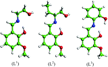 |
| | Fig. 1 Molecular structures of the synthesized Schiff bases. | |
2-((2-Hydroxyethylimino)methyl)-6-methoxyphenol (L1)
Yield: 88%. Elemental analysis: anal. calcd: C, 61.53; H, 6.71; N, 7.18. Found: C, 61.05; H, 6.19; N, 6.91%. Characteristic IR peaks (KBr disk): νO–H = 3420,29νC–H = 3080,30νC–H(methoxy) = 2830,30νC![[double bond, length as m-dash]](https://www.rsc.org/images/entities/char_e001.gif) N = 1650,30νCC = 1500,12νC–O = 1175 cm−1
N = 1650,30νCC = 1500,12νC–O = 1175 cm−1![[thin space (1/6-em)]](https://www.rsc.org/images/entities/char_2009.gif) 30,31 (Fig. S1, ESI†); ESI-MS [L1 + H+]: m/z 196.3 amu (Fig. S4, ESI†); 1H-NMR (300 MHz, DMSO-d6, Me4Si, δH, ppm): 13.821 (br-s, 1H, Ar-OH), 8.482 (s, 1H, –CHN–), 6.995–7.014 (d, 2H, Ar-H), 6.740–6.779 (t, 1H, Ar-H), 4.816 (s, 1H, R–OH), 3.773 (s, 3H, Ar-OCH3), 3.649 (m, 4H, –N(CH2)2–) (Fig. S7, ESI†) and 13C-NMR (300 MHz, DMSO-d6, δC, ppm) (Fig. S10, ESI†).
30,31 (Fig. S1, ESI†); ESI-MS [L1 + H+]: m/z 196.3 amu (Fig. S4, ESI†); 1H-NMR (300 MHz, DMSO-d6, Me4Si, δH, ppm): 13.821 (br-s, 1H, Ar-OH), 8.482 (s, 1H, –CHN–), 6.995–7.014 (d, 2H, Ar-H), 6.740–6.779 (t, 1H, Ar-H), 4.816 (s, 1H, R–OH), 3.773 (s, 3H, Ar-OCH3), 3.649 (m, 4H, –N(CH2)2–) (Fig. S7, ESI†) and 13C-NMR (300 MHz, DMSO-d6, δC, ppm) (Fig. S10, ESI†).
2-((1-Hydroxybutan-2-ylimino)methyl)-6-methoxyphenol (L2)
Yield: 92%. Elemental analysis: anal. calcd: C, 64.55; H, 7.67; N, 6.27. Found: C, 64.21; H, 7.43; N, 6.21. Characteristic IR peaks (KBr disk): νO–H = 3395,29νC–H = 3035,30νC–H(methoxy) = 2830,30νCN = 1650,30νCC = 1500,12νC–O = 1180 cm−130,31 (Fig. S2, ESI†); ESI-MS [L2 + H+]: m/z 224.4 amu (Fig. S5, ESI†); 1H-NMR (300 MHz, DMSO-d6, Me4Si, δH, ppm): 13.909 (br-s, 1H, Ar-OH), 8.476 (s, 1H, –CHN–), 7.011–7.041 (m, 2H, Ar-H), 6.764–6.803 (t, 1H, Ar-H), 4.816 (s, 1H, R–OH), 3.778 (s, 3H, Ar-OCH3), 3.426–3.587 (m, 2H, R–CH2OH), 3.180–3.210 (m, 1H, N–CH), 1.526–1.663 (m, 2H, R–CH2–), 0.827–0.864 (m, 3H, R–CH3) (Fig. S8, ESI†) and 13C-NMR (300 MHz, DMSO-d6, δC, ppm) (Fig. S11, ESI†).
2-(2-Hydroxy-3-methoxybenzylideneamino)phenol (L3)
Yield: 90%. Elemental analysis: anal. calcd: C, 69.12; H, 5.39; N, 5.76. Found: C, 68.93; H, 5.24; N, 5.57. Characteristic IR peaks (KBr disk): νO–H = 3410,29νC–H = 3055,30νC–H(methoxy) = 2825,30νCN = 1635,30νCC = 1495,12νC–O = 1190 cm−130,31 (Fig. S3, ESI†); ESI-MS [L3 + H+]: m/z 244.3 amu (Fig. S6, ESI†); 1H-NMR (300 MHz, DMSO-d6, Me4Si, δH, ppm): 14.080 (s, 1H, Ar-OH), 9.792 (s, 1H, Ar′-OH), 8.966 (s, 1H, –CHN–), 7.134–7.152 (d, 1H, Ar-H), 7.094–7.096 (d, 1H, Ar-H), 6.965–6.985 (m, 1H, Ar-H), 3.816 (s, 3H, Ar-OCH3), 7.375–7.395 (m, 1H, Ar′-H), 7.182–7.204 (m, 1H, Ar′-H), 7.113–7.117 (d, 1H, Ar′-H), 6.860–6.865 (d, 1H, Ar′-H) (Fig. S9, ESI†) and 13C-NMR (300 MHz, DMSO-d6, δC, ppm) (Fig. S12, ESI†).
Specimens and solution
Cylindrical shaped, commercially available mild steel rods (wt% composition: 0.22 C, 0.31 Si, 0.60 Mn, 0.04 P, 0.06 S and the remainder Fe) were taken as test specimens. Prior to each experiment, the cross-section of the sample was polished using metallurgical grade emery paper of 400 to 1600 grade. These were then washed thoroughly with ethanol and double distilled water and were used as the working electrode in electrochemistry. Here, for the preparation of 1 M HCl solution, GR grade HCl (35%) obtained from Merck, India was used.
Electrochemical measurements
Electrochemical studies (potentiodynamic polarization and electrochemical impedance spectroscopy) were carried out using conventional three-electrode cell systems consisting of mild steel specimens as the working electrode (WE) with 1 cm2 surface area (cover one side), platinum and saturated calomel electrode (SCE) as the counter and reference electrodes, respectively. Before each and every individual experiment, WE was dipped into the test solution for 20 minutes to establish a stable open circuit potential (OCP) and OCP was monitored for the next 30 minutes (Fig. S13, ESI†). No such significant deviation in the OCP (vide Fig. S13, ESI†) confirmed that the steady state was reached. Potentiodynamic polarization measurements were carried out by polarizing the specimens with a scan rate of 0.5 mV s−1 in the potential range of ±250 mV with respect to the OCP. In this experiment, corrosion current density (icorr) was determined by the extrapolation of cathodic and anodic Tafel curves to the corrosion potential Ecorr. Electrochemical impedance spectroscopy measurements were performed in the frequency range of 100 kHz to 10 MHz using an AC amplitude of 10 mV at the OCP. All the experiments were carried out under unstirred conditions at around 27 °C (room temperature).
Weight loss measurement
The weight loss experiments were carried out using mild steel rectangular coupons (wt% composition: 0.19 C, 0.21 Si, 0.21 Mn, 0.01 P, 0.01 S and the remainder iron) having dimensions of 2.5 cm × 2.5 cm × 0.1 cm. Before the weight loss experiments, the coupons were polished with different grades of emery papers (400–1600 grade), followed by washing thoroughly with acetone and distilled water and were finally dried in desiccators. The weight loss measurements were studied on mild steel samples dipped into 1 M HCl medium in the absence and presence of inhibitor molecules having the optimum concentration of 5 mM for 2–96 h at room temperature (∼27 °C). The percentage of inhibition efficiency was calculated according to the following relation:| | 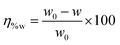 | (1) |
where w0 and w are the weight loss of mild steel coupons immersed in an acidic medium in the absence and presence of inhibitors for the same immersion time. In the present investigation, all the electrochemical and gravimetric experiments were repeated thrice and the results obtained from these different sets of experiments are found to be very close (within ±1 to 2%).
Surface morphology
Prior to the morphology study, the metallic specimens were prepared by keeping polished mild steel coupons in 1 M HCl medium for 6 h in the absence and presence of inhibitors having 5 mM concentration. The specimens were then taken out from the test solution, washed gently with distilled water followed by acetone, and then carefully dried. Thereafter, the surface-prepared mild steel specimens were analyzed using field emission scanning electron microscopy (FESEM). With the aim of representing a constant view, the morphologies of all the corroded specimens were recorded at the magnification of ×5000.
Computational details for density functional theory calculations
In order to correlate the molecular properties of the inhibitors with the corrosion inhibitive performances, density functional theory (DFT) has been employed. Herein, the ORCA programme package, 2.7.0 version has been used for all DFT calculations.32 The B3LYP functional level of DFT has been employed for geometry optimization of the inhibitor molecules.33–37 All-electron Gaussian basis sets were developed by the Ahlrichs group.38 In this investigation, the triple-ζ quality basis set TZV(P) along with one set of polarization functions on the N, O heteroatoms are used.39 For smaller atoms like carbon and hydrogen, slightly smaller polarized split-valence SV(P) basis sets are used, which are of double-ζ quality in the valance region and have a polarizing set of d functions on the non-hydrogen atoms. Self-consistent fields (SCF) were converged tightly with [1 × 10⁻⁷Eh: density change, 1 × 10⁻⁸Eh: energy, 1 × 10⁻⁷: the maximum element of the DIIS error vector]. In this investigation, all the calculations were executed in the aqueous phase, since solution state metallic corrosion always happens in the liquid phase. The solvent effect (water) was introduced by the utilization of the COSMO model during the simulation process.
Computational details for density functional tight binding calculations
An insightful study of the interactions between the inhibitor molecule and metal surface was performed by the density functional tight binding (DFTB) method. DFTB is an approximation of the Kohn–Sham density functional theory employing a parameterized Hamiltonian matrix.40–42 The accuracy of this method largely depends on the parameters (Slater–Koster library set) used in the calculation. The DFTB method has become popular due to its computational efficiency and accuracy. This method considerably reduces the computational cost and is able to achieve both ground state and excited state properties of the molecules.
Before starting the calculations, we had to decide which surface of iron would be chosen for the entire calculations. In this regard, it is worth mentioning that we employed the “morphology” module in the Material Studio software (version 6.1) for the selection of the appropriate adsorption surface.43 The calculations indicate that the Fe(110) surface has a densely packed surface and lower surface energy. Therefore, the Fe(110) surface was chosen for inhibitor–metal interactions in the DFTB method. Four atomic layers of iron were used to construct the iron slab. Thereafter, the unit cell was extended to the x and y directions with the supercell of 7 × 7. Finally, a vacuum layer of 30 Å thickness was built over the iron surface.
In this investigation, all the calculations were employed using the DFTB+ program package available in Material Studio™ software (version 6.1).43 The trans3d Slater–Koster library set was used for the possible pairs of interactions between C, N, O, H and Fe. Geometry optimization was tightly converged [0.01 kcal mol−1 energy, 0.1 kcal mol−1 Å−1 force and 0.001 Å displacement]. Self-consistent charge (SCC) tolerance was set to 10−8 a.u. elementary charge. To reduce the number of SCC iterations, Broyden mixing was used.44,45 All the calculations were carried out with the k-points of 4 × 4 × 1. During the calculation, the bottom two layers of the iron slab were kept frozen to their ideal crystalline positions, whereas the upper half of the slab with the inhibitor molecule was fully relaxed.
The adsorption energy (Eads) between the Fe(110) surface and the inhibitor molecule can be calculated as follows:44
| | | Eads = Ecomplex − (Esurface + Einhibitor) | (2) |
where
Ecomplex is the total energy of the system,
Esurface represents the total energy of the iron slab, and
Einhibitor is defined as the energy of a surface-adsorbed form of the inhibitor molecule.
Computational details for molecular dynamics simulation
In recent times, MD simulation has emerged as a widely accepted simulation technique where preferential adsorption sites of the inhibitor molecules on the metallic surfaces can be envisaged. In this investigation, MD simulation was carried out by employing the discover module Material StudioTM software version 6.1 (from Accelrys Inc.).43 Here, the Fe(110) surface has been chosen for the simulation study as it has a packed surface and better stabilization energy. The interactions between the inhibitor molecules and Fe(110) surface have been performed in a modelled simulation box (dimension: 39.6 × 39.6 × 75.8 Å) with periodic boundary conditions. Herein, the whole simulation box was constructed by using three layers. The lowest layer was the iron slab (constructed by the 10 layers of Fe atoms), the middle layer was the solution slab (contains studied inhibitor molecule, H2O molecules and molecular ions like H3O+, Cl−) and the remaining uppermost layer was the vacuum layer. The Condensed Phase Optimized Molecular Potentials for Atomistic Simulation Studies (COMPASS) force field has been used for all the dynamic simulations. COMPASS is a highly accepted ab initio force field that facilitates the precise prediction of chemical properties for various molecules or compounds.46 The functional form of the COMPASS force field is expressed as follows:47,48| | | E = Ebond + Eangle + Eoop + Etorsion + Ecross + Eelec + Elj | (3) |
where Ebond is the contribution of bond stretching, Eangle is due to angle bending, Eoop refers to out of plane angle coordinates, Etorsion is the effect of torsion, Ecross implies the coupling, Eelec and Elj symbolize the electrostatic and van der Waals interactions, respectively. A detailed description of each term in eqn (3) has been shown in eqn (S1) of the ESI† of the manuscript.
During the entire dynamic simulations, bulk Fe atoms were kept “frozen” and all the concerned species were allowed to freely interact with the metal surface. In this particular investigation, MD simulations have been carried out by incorporating the NVT canonical ensemble at 300 K with a time step of 1.0 fs and simulation period of 200 ps.
The interaction energy (Einteraction) between the Fe(110) surface and the inhibitor molecule can be calculated as follows:43
| | | Einteraction = Etotal − (Esurface+H2O+H3O++Cl− + Einhibitor) | (4) |
where the total energy of the simulation system is defined as
Etotal, the energy of the iron surface together with H
2O, H
3O
+, Cl
− is classified as
Esurface+H2O+H3O++Cl−, and the single point energy of the surface adsorbed form of the inhibitor molecule is defined as
Einhibitor.
The negative value of the interaction energy gives the binding energy of the inhibitor molecule:12,14
| | | Ebinding = −Einteraction | (5) |
Results and discussion
Potentiodynamic polarization
The current–potential relationships for a mild steel electrode in 1 M HCl medium without and with inhibitors having 5 mM concentration are presented in Fig. 2. Such polarization curves for individual inhibitor molecules having different inhibitor concentration (0.5 mM to 5 mM) are plotted in the ESI† (Fig. S14). Different parameters obtained from the polarization study such as corrosion potential (Ecorr), anodic Tafel slope (βa), cathodic Tafel slope (βc) and corrosion current density (icorr) are shown in Table 1. The percentage of inhibition efficiency (η%P) for different inhibitor concentrations is determined as follows:| | 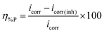 | (6) |
where, icorr and icorr(inh) are corrosion current densities without and with the application of inhibitor, respectively.
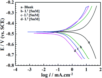 |
| | Fig. 2 Potentiodynamic polarization curves for mild steel in 1 M HCl solution in the absence and presence of Schiff bases (L1, L2 and L3) having 5 mM concentration. | |
Table 1 Potentiodynamic polarization parameters and percentage of corrosion inhibition efficiency obtained for mild steel in 1 M HCl medium in absence and presence of different concentration of three Schiff base inhibitors
| System |
Conc. (mM) |
−Ecorr (mV/SCE) |
i
corr (μA cm−2) |
β
a (mV dec−1) |
β
c (mV dec−1) |
η
%P
|
| 1 M HCl |
Blank |
480 |
5792 |
218.4 |
256.1 |
— |
|
|
| L1 |
0.5 |
487 |
2074 |
127.4 |
195 |
64.2 |
| 1 |
480 |
1277 |
132.4 |
190.1 |
77.9 |
| 2.5 |
479 |
672 |
109.6 |
162.7 |
88.4 |
| 5 |
480 |
502 |
112.7 |
164.3 |
91.3 |
|
|
| L2 |
0.5 |
480 |
1375 |
122.5 |
167.0 |
76.3 |
| 1 |
487 |
925 |
127.6 |
169.9 |
84.0 |
| 2.5 |
489 |
455 |
107.7 |
160.8 |
92.1 |
| 5 |
482 |
323 |
120.9 |
181.2 |
94.4 |
|
|
| L3 |
0.5 |
480 |
929 |
90.3 |
161.5 |
83.9 |
| 1 |
482 |
538 |
88.1 |
156.8 |
90.7 |
| 2.5 |
492 |
376 |
94.2 |
163.2 |
93.5 |
| 5 |
495 |
181 |
99.5 |
166.5 |
96.8 |
From Fig. 2 and Table 1 it can be seen that the presence of inhibitor molecules in the aggressive acidic medium significantly reduces anodic as well as cathodic current densities, which suggests that both the anodic dissolution of mild steel and cathodic hydrogen ion reduction have been inhibited. Thus, inhibitor molecules act as mixed-type inhibitors.
The classification of inhibitors as cathodic, anodic or mixed-type can also be determined from the Ecorr values. The inhibitor molecules are categorized as cathodic or anodic types when the difference between Ecorr values without and with inhibitors is greater than 85 mV.12,49 For the present investigation, Table 1 shows that the displacement of the Ecorr values of the synthesized inhibitor molecules assembled on the surfaces of mild steel is less than 85 mV. Hence, it implies that the studied Schiff base molecules behave as the mixed-type inhibitors.50 Furthermore, in the presence of inhibitors, the negative shifting of the Ecorr values reveals that the inhibitor molecules produce more beneficial effects on the H+ ion reduction (cathodic reaction) than that of the mild steel dissolution reaction (anodic reaction). Thus, it is concluded from this observation that all the presently investigated inhibitor molecules possess mixed-type inhibition properties with predominantly cathodic inhibitive nature.
Table 1 shows a remarkable decrease in icorr values in the presence of inhibitor molecules. It is also observed that the corrosion current density for the entire inhibitor concentrations (from 0.5 mM to 5.0 mM) decreased in the order of L3 > L2 > L1. Such a trend of inhibition efficacy is successfully elucidated on the basis of the molecular structure consideration of these inhibitor molecules. From the molecular structures of the inhibitor molecules (Fig. 1) it has been found that in the L1 ligand, one aromatic moiety is coupled with one small aliphatic chain by a simple azomethine linkage. Hence, the inhibitor molecule possesses many heteroatoms, unsaturated π-electrons and azomethine groups in its structure. Based on these cumulative effects, the ligand L1 has shown admirable corrosion inhibition capability. It is interesting to see that when the aliphatic chain (i.e., the 2-aminoethanol part) of the L1 ligand was replaced by branched 2-aminobutan-1-ol for the formation of the L2 inhibitor, the corrosion inhibition efficiency of the molecule was increased. This may be explained by the fact that the additional branching chain comprised of the –C2H5 group (which has electron donation capability, +I effect) moderately enhances the electron density over the molecular skeleton of the inhibitor molecule; therefore, the adsorption ability of the inhibitor molecule is increased. Very interestingly, it is also seen that when the aliphatic chain of the L2 ligand is replaced with the aromatic moiety forming L3, the inhibition property is further increased. This may also be explained by the higher chemisorption ability of aromatic moieties. From this, it can be concluded that for the small aliphatic chains and the aromatic moiety, the latter obviously has a greater propensity towards the adsorption process. Furthermore, these factual experimental outcomes have been well explained with the aid of quantum chemical calculations as well as MD simulations.
Electrochemical impedance spectroscopy
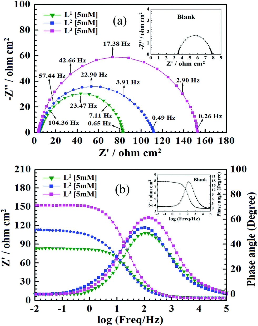
With the aim of understanding the kinetics and characteristics of the electrochemical process on the mild steel surface in the acidic media and to get a better insight into the mechanism of corrosion inhibition, EIS measurements were performed. EIS is a non-destructive technique that is used for the rapid characterization and study of corrosion inhibition behaviour. For mild steel, Nyquist plots obtained from EIS studies in the absence and presence of inhibitors having 5 mM concentration are shown in Fig. 3, and Nyquist plots for all three inhibitors with varying inhibitor concentration (0.5 mM to 5 mM) are presented in Fig. S15 (ESI†).
 |
| | Fig. 3 (a) Nyquist impedance diagram. (b) Bode plots for mild steel in 1 M HCl solution in the absence and presence of Schiff bases (L1, L2 and L3) having 5 mM concentration. Inset: Nyquist diagram and Bode plot in the absence of inhibitors (blank). | |
It is observed from Fig. 3 that in the absence of inhibitors, the Nyquist plots consist of only one semicircle and one time constant in the bode plots (Fig. 3b), which suggest that the dissolution of mild steel in 1 M HCl is mainly controlled by the charge transfer process. In the Nyquist plot, the difference in the higher and lower frequencies in real impedance is usually defined as the charge transfer resistance (Rct). This resistance must correspond to the resistance between the metal and the outer Helmholtz plane (OHP).12,14,51 Thus, in the absence of inhibitors, the resistance exhibited at the metal/solution interface is mainly due to the charge transfer resistance (Rct), accumulation resistance (Ra) and diffuse layer resistance (Rd). As a result, along with Rct, Ra and Rd have to be considered. Therefore, the difference in the real impedance at lower and higher frequency is considered the polarization resistance (Rp).12,14,51
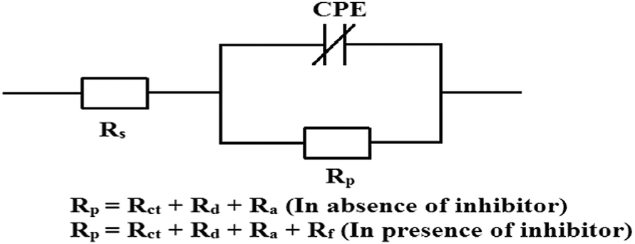
It is seen that after the addition of inhibitors, the diameter of the semicircle in the Nyquist plot is concomitantly increased. This suggests the formation of a protective layer on the mild steel surfaces. Therefore, in the presence of inhibitors, film resistance (Rf) has to be added to the polarization resistance (Rp); thus, polarization resistance (Rp) in the presence of inhibitors is designated as ∑(Rct + Rd + Ra + Rf).12,14,51,52 Closer inspection of the Nyquist plots reveals that the obtained semicircles are depressed under the real axis, which may be attributed to the microscopic roughness and inhomogeneity of the electrode surface.14,16 With this in mind, to get more accurate results, the constant phase element (CPE) was incorporated in the equivalent circuit (Fig. 4).
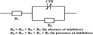 |
| | Fig. 4 The electrical equivalent circuit used to fit the EIS experimental data. | |
The obtained Nyquist plots were fitted with the equivalent circuit as depicted in Fig. 4, where CPE is parallel to Rp and this combination is connected in series with the electrolyte resistance (Rs). CPE is associated with double layer capacitance (Cdl) and the corresponding impedance is determined with the help of following equation:53,54
where
Q is a proportionality coefficient,
ω is the angular frequency, i is the imaginary unit and
n is a measure of surface irregularity. For whole numbers of
n = −1, 0, 1, CPE represents inductance (
L), resistance (
R) and capacitance (
C), respectively.
To obtain a direct correlation between polarization resistance (Rp) and double layer capacitance (Cdl), the latter has been recalculated by using the following equation:53
The fitted electrochemical impedance parameters obtained from the Nyquist plots are tabulated in
Table 2. Inspection of the results in
Table 2 reveals that with increasing inhibitor concentrations, the polarization resistance (
Rp) is concomitantly increased whereas the
Cdl values are reversely dependent. This is probably due to the increase in surface coverage on the mild steel surface by the adsorption of inhibitor molecules, leading to better inhibition efficiencies. The decrease in
Cdl values reflects the reduction of the local dielectric constant, which is attributed to the adsorption of inhibitor molecules on the metal surface by replacing pre-adsorbed water molecules and/or an increase in the thickness of the electric double layer. The obtained outcome manifests that inhibitor molecules act by adsorption on the metal/solution interface.
Table 2 EIS parameters and the percentage of corrosion inhibition efficiency obtained for mild steel in 1 M HCl medium in the absence and presence of different concentrations of three Schiff base inhibitors
| System |
Conc. (mM) |
R
s (Ω cm2) |
R
p (Ω cm2) |
Q (μΩ−1 sn cm−2) |
C
dl (μF cm−2) |
n
|
η
%Z
|
θ
|
| 1 M HCl |
Blank |
3.477 |
4.35 |
1154 |
378 |
0.826 |
— |
— |
|
|
| L1 |
0.5 |
4.835 |
12.97 |
738 |
312 |
0.844 |
66.5 |
0.665 |
| 1 |
3.642 |
32.48 |
607 |
247 |
0.814 |
86.6 |
0.866 |
| 2.5 |
3.745 |
49.8 |
527 |
188 |
0.780 |
91.3 |
0.913 |
| 5 |
4.5 |
77.64 |
235 |
87 |
0.803 |
94.4 |
0.944 |
|
|
| L2 |
0.5 |
3.798 |
25.54 |
627 |
264 |
0.827 |
82.9 |
0.829 |
| 1 |
4.037 |
47.71 |
543 |
241 |
0.818 |
90.9 |
0.909 |
| 2.5 |
4.039 |
70.32 |
431 |
181 |
0.802 |
93.8 |
0.938 |
| 5 |
4.019 |
105.4 |
195 |
72 |
0.796 |
95.9 |
0.959 |
|
|
| L3 |
0.5 |
3.627 |
39.05 |
432 |
158 |
0.803 |
88.9 |
0.889 |
| 1 |
3.634 |
63.79 |
304 |
134 |
0.828 |
93.2 |
0.932 |
| 2.5 |
3.578 |
94.44 |
207 |
90 |
0.826 |
95.4 |
0.954 |
| 5 |
3.499 |
149.8 |
132 |
67 |
0.855 |
97.1 |
0.971 |
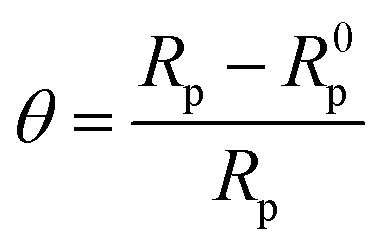
The extent of surface coverage (θ) and the percentage inhibition efficiency (η%Z) of the inhibitor molecules on the metallic surface are determined by the following expressions:
| |  | (9) |
| |  | (10) |
where
Rp and
R0p represent the polarization resistance in the presence and absence of inhibitor molecules, respectively. An evaluation of
Table 2 reveals that the percentage of inhibition efficiency, calculated in terms of polarization resistance (
Rp), follows the order of L
3 > L
2 > L
1. These outcomes are consistent with the results obtained from the potentiodynamic polarization study. Thus, the outcome obtained from the EIS study gives the same result that the aromatic moiety has better adsorption capability compared to the small aliphatic chains.
Adsorption isotherm and thermodynamics parameters
The adsorption isotherm is extensively applied for exploring the adsorption behaviour of the studied inhibitor molecules on the desired surfaces of metals. The inhibitor molecules adsorb on the metallic surfaces by displacing the water molecules surrounding the corroding interface. The adsorption of inhibitor molecules on the electrode surface is a quasi-substitution process between the inhibitor molecule in the aqueous phase and water molecules at the electrode surface.55,56 The displacement of water molecule by the inhibitor molecule can be represented as follows:| | | Inh(sol) + xH2O(ads) ↔ Inh(ads) + xH2O(sol) | (11) |
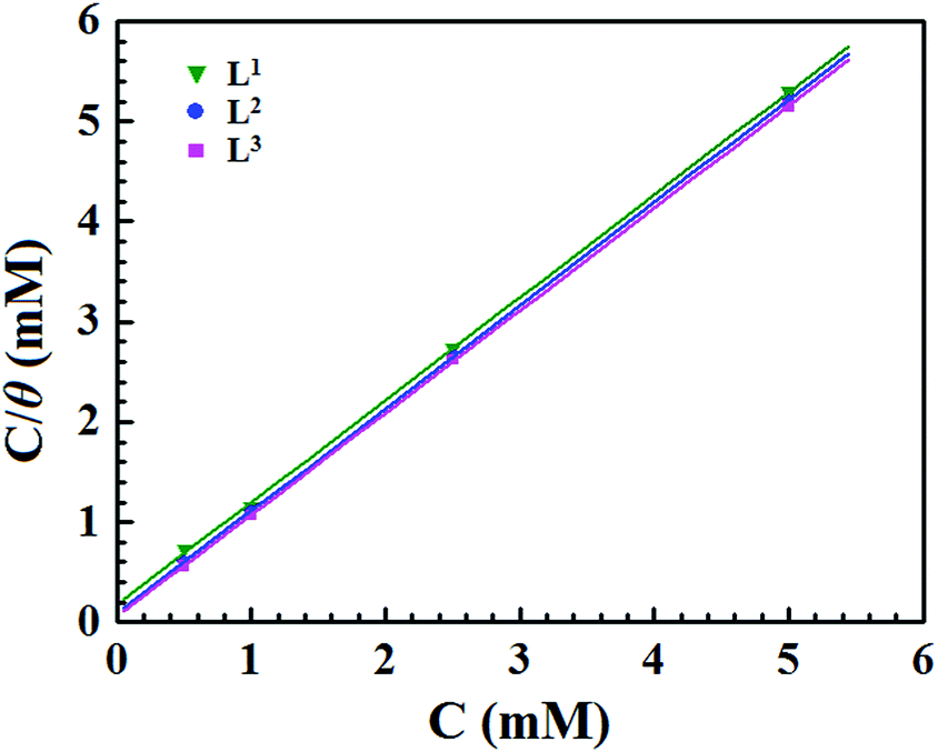
where Inh(sol) and Inh(ads) are the inhibitor molecules in the solution and adsorbed in the electrode surface, respectively, and x is the number of water molecules displaced by the organic inhibitor. In this investigation, several kinds of adsorption isotherms, such as the Langmuir, Temkin, Frumkin isotherms, etc., were used to elucidate the adsorption behaviour of the synthesized Schiff base inhibitor molecules. Herein, EIS data are utilized for fitting several adsorption isotherms. It was observed that the most suitable fitting of the EIS data follows the Langmuir adsorption isotherm. Based on this adsorption isotherm, the relationship between the degree of surface coverage (θ) and the concentration of the inhibitor (C) is related by the following equation:12,14,57where Kads is the equilibrium adsorption constant. Langmuir adsorption isotherm plots (Fig. 5) of the three synthesized inhibitor molecules give straight lines with strong correlation coefficients (R2 = 0.999). This indicates that the studied inhibitor molecules obeyed the Langmuir adsorption isotherm.
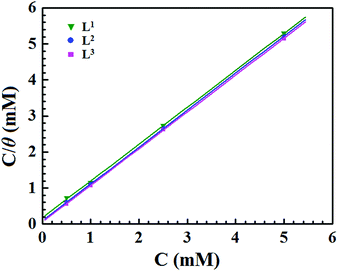 |
| | Fig. 5 Langmuir adsorption plots for mild steel in acidic media containing different concentrations of Schiff bases. | |
The equilibrium adsorption constant (Kads) is associated with the standard free energy of adsorption (ΔG0ads) by the following equation:12,14,57
| |  | (13) |
where 55.5 is the molar concentration of water,
R is the universal gas constant and
T is the absolute temperature. The obtained Δ
G0ads values of the three studied inhibitors are given in
Table 3.
Table 3 Adsorption parameters of Schiff base ligands on mild steel in 1 M HCl
| Inhibitors |
R
2
|
Slope |
K
ads (M−1) |
−ΔGads (kJ mol−1) |
| L1 |
0.99977 |
1.019 |
5.23 × 10³ |
31.37 |
| L2 |
0.99999 |
1.026 |
11.61 × 10³ |
33.36 |
| L3 |
0.99999 |
1.019 |
17.49 × 10³ |
34.38 |
In general, ΔG0ads values of around −20 kJ mol−1 or less negative are associated with the electrostatic interaction between the charged inhibitor molecules and charged metal surfaces (physisorption type). The ΔG0ads values around −40 kJ mol−1 or more negative are commonly interpreted with the charge sharing or transfer between the inhibitor molecules and metal surfaces to form a coordinate type of bond (chemisorption type).58–60 It can be seen from Table 3 that the obtained ΔG0ads values of the synthesized inhibitor molecules lie in the order of −31.37 to −34.38 kJ mol−1. The negative value of ΔG0ads indicates the spontaneous adsorption of the Schiff base molecules on the mild steel surface. The above range of ΔG0ads values also suggest that a mixed type of adsorption by the studied inhibitor molecules occurs, which means that physisorption and chemisorption occur on the mild steel surface in 1 M HCl medium.
It can be seen from Table 3 that when the aromatic moiety is coupled with a small aliphatic chain by the azomethine linkage, it shows a ΔG0ads value of −31.37 kJ mol−1. The obtained ΔG0ads value suggests that this molecule has both the physisorption and chemisorption properties. However, the chemisorption properties are predominant. It is interesting that when the aliphatic chains were branched for the preparation of L2, the free energy of adsorption also increased, which suggests that the chemisorption properties of the molecule were increased. Therefore, it could be said that due to the additional branching chain of the ligand L2, the chemisorption properties of the molecule are enhanced. It is also noticed that the additional branching chain is comprised of the –C2H5 group, which has electron donation capability (+I effect) and thereby enhances the electron density over the molecular skeleton of the inhibitor molecule; thus, the adsorption capability of the inhibitor molecule was increased. For this reason, the L2 inhibitor molecule has greater ΔG0ads value in comparison to the L1 inhibitor. Very interestingly, it is seen that when the aliphatic chain in the L2 ligand is replaced by the aromatic moiety forming L3, the ΔG0ads value is further increased. Thus, it is concluded that among the aromatic moieties and small aliphatic chains, the aromatic moiety has a greater donor–acceptor (D–A) capability than that of small aliphatic chains. For this reason, the L3 inhibitor has a higher binding capability on the mild steel surface and thus the corrosion inhibition efficiency is higher compared to the other two inhibitor molecules.
Weight loss measurements
The anti-corrosive behaviour of the Schiff base molecules was further corroborated by the weight loss method. The weight loss method is very useful due to its good reliability. The variation in the percentage of inhibition efficiency with an immersion time of 2–96 h for mild steel specimens in 1 M HCl solution in the presence of inhibitor molecules having 5 mM concentration is shown in the ESI† (Fig. S16). It can be seen from Fig. S16 (ESI†) that the percentage inhibition efficiency (η%W) increases with increasing immersion time and attains a maximum value of 86%, 90% and 94% for L1, L2 and L3, respectively. The increasing inhibition efficiency with increasing immersion time (2–96 h) can be explained in terms of the extent of surface coverage by the inhibitor molecule on the metallic surfaces. A two-dimensional layer was formed on the metallic surface and therefore η%W increases with increasing immersion time. It was also seen that for the whole range of immersion time, the inhibition efficiency increases in the order of L3 > L2 > L1. This outcome also suggests that the L3 inhibitor has better adsorption capability compared to the L2 and L1. The adsorption capability has also been explained in terms of D–A capability as well as the electrostatic interaction between the inhibitor molecule and the mild steel surface. A keen observation of the molecular structure of the inhibitor shows that all the molecules have more or less the same number of protonation sites. Thus, it can be stated that electrostatic interaction does not create any variation in the inhibition efficiencies of the inhibitor molecules. Therefore, the variation in inhibition efficiency has to be related to the D–A capability of the molecule, i.e., the chemisorption properties of the molecule. In the adsorption isotherm section, it has already been elaborately discussed that of the small aliphatic chain, the branched aliphatic chain and aromatic moiety, the greatest adsorption ability was observed for the aromatic moiety of the molecule. Since one part of the molecular framework was varied from the small aliphatic to the branched aliphatic and finally, to the aromatic moiety, the D–A capability of the inhibitor molecule was increased. For this reason, L3 shows higher adsorption ability than that of L2, and L2 is higher than that of L1; this has been discussed elaborately by theoretical analysis.
Surface morphology study
FESEM/EDX analysis.
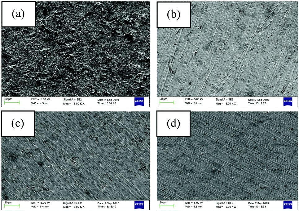
The morphologies of the metallic surfaces in the absence and presence of inhibitor in 1 M HCl medium have been analyzed by FESEM. In addition, the elemental content present in the corrosion related specimens was also analyzed by the EDX study. The obtained FESEM images of mild steel specimens immersed in 1 M HCl for the duration of 6 h in the absence and presence of the inhibitors having 5 mM concentration are depicted in Fig. 6, where it can be seen (Fig. 6a) that the mild steel surface is highly corroded and damaged in absence of inhibitors. In the absence of inhibitors, there were several mountainlike appearances, which indicate the direct attack of aggressive acidic ions. On the other hand, in the presence of inhibitors (videFig. 6b–d), a relatively cleaner and smoother surface was observed. This indicates that a protective film was formed on the mild steel surface. The formed protective film isolates the surfaces of metallic bodies from the aggressive acidic attack and thereby ensures a less corroded surface.
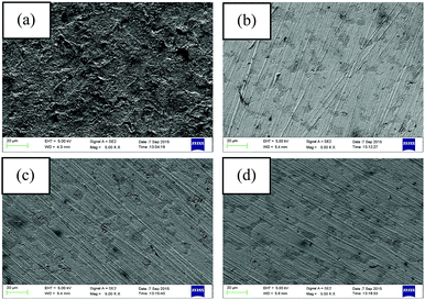 |
| | Fig. 6 FESEM images of mild steel surfaces after 6 h immersion in 1 M HCl medium with (a) no inhibitor, (b) 5 mM L1, (c) 5 mM L2 and (d) 5 mM L3 (magnification, ×5000). | |
In order to further confirm whether inhibitors are adhering on the metallic surfaces or not, EDX analysis was also employed. The obtained EDX spectra in the absence and presence of inhibitors are shown in Fig. S17 (ESI†). The presence of chloride in all the EDX spectra of mild steel reveals that the mild steel surface has been exposed to the acidic solution. In absence of inhibitors (Fig. S17a, ESI†), apart from the elemental content of mild steel and chlorine atoms, no additional signals were observed; whereas, in the presence of inhibitors (Fig. S17b–d, ESI†) additional nitrogen and oxygen signals appeared in the EDX spectrum. These additional signals in the EDX spectrum suggest that inhibitor molecules definitely adhered to the metallic surfaces.
AFM measurement
AFM analysis was performed after 6 h of immersion of the mild steel specimens in 1 M HCl medium in the absence and presence of the maximum concentration of inhibitors. The obtained AFM micrographs are depicted in Fig. 7. It can be seen from Fig. 7a that the mild steel surface immersed in 1 M HCl medium without inhibitors was highly corroded and enormous mountain-like peaks appeared. This is associated with the direct exposure of the mild steel surfaces to the acidic media. Here, aggressive ions directly attack the mild steel surfaces and thereby destroy the whole surfaces. The average surface roughness calculated for the mild steel surface in the blank acidic medium was 308 nm. On the other hand, the AFM micrograph of the mild steel surfaces in the presence of the maximum concentration of inhibitors shows significant improvement of the smoothness of the surface. This phenomenon can be explained in terms of the adsorption of inhibitor molecules on the metallic surfaces. The obtained average surface roughness of the mild steel surfaces in the presence of L1, L2 and L3 inhibitors is 144 nm, 130 nm and 40 nm, respectively. Thus, from the roughness values in the absence and presence of inhibitors, it can be concluded that our synthesized inhibitor molecules definitely work in the aggressive acidic medium.
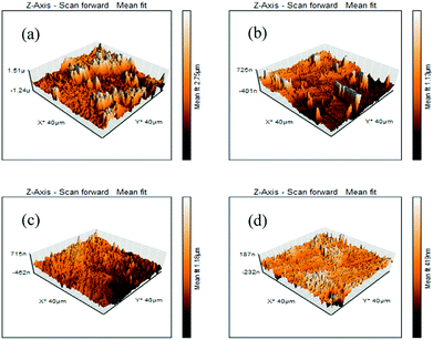 |
| | Fig. 7 AFM images of mild steel surfaces after 6 h immersion in 1 M HCl medium with (a) no inhibitor, (b) 5 mM L1, (c) 5 mM L2 and (d) 5 mM L3. | |
Contact angle measurement
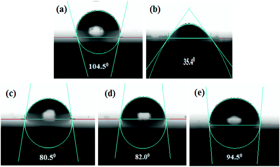
It is also possible to determine the effectiveness of the corrosion inhibitors in the acidic medium from the water contact angle measurement. When inhibitor molecules are adsorbed on the mild steel surface, the chemical composition of the metal surface is changed and the wettability of the surface is also changed. Therefore, the characteristics of the mild steel surface (i.e., the hydrophilic or hydrophobic properties) in the presence and absence of inhibitors can be directly determined by the water contact angle measurement. Here, the wetting characteristics of the mild steel surfaces were analyzed after 6 h immersion in the 1 M HCl medium in the absence and presence of the maximum concentration of inhibitors. All the measured contact angles between a water droplet and mild steel specimens are depicted in Fig. 8; the freshly polished mild steel specimen served as a reference (Fig. 8a). The freshly polished mild steel surface showed water repellent characteristics with a contact angle of 104.5°.61 In contrast, when the mild steel specimen was immersed in 1 M HCl medium for 6 h, the contact angle was found to be decreased to 35.4° (videFig. 8b). This hydrophilic property is mainly associated with the formation of corrosion product on the mild steel surfaces. Since the formed corrosion products are mainly polar in nature, they modify the composition and properties of the surfaces. For this reason, water droplets are easily deformed on the surfaces. In contrast, it is also seen that after the addition of inhibitor molecules in the aggressive acidic solution, the contact angle was increased. In the presence of 5 mM concentration of L1, L2 and L3 inhibitors, the contact angles were modified to 80.5°, 82.0° and 94.5°, respectively, suggesting that a water-repellent film was formed on the mild steel surfaces in the presence of inhibitors in the aggressive acidic media; as a result, the hydrophilic surface was moved into the hydrophobic surface in the presence of inhibitor molecules in the acidic media. It was also established once again that between the small aliphatic chains and aromatic moiety, the aromatic moiety obviously has better surface protecting capability than the small aliphatic chains.
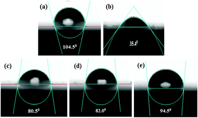 |
| | Fig. 8 Water contact angle measurement on (a) the polished mild surface and after 6 h of immersion in 1 M HCl medium with (b) no inhibitor, (c) 5 mM L1, (d) 5 mM L2, (e) 5 mM L3. | |
Density functional theory calculations
In recent times, quantum chemical calculations have been treated as an effective tool for the design and development of several potential corrosion inhibitor molecules. DFT analyses of each and every molecule can be conducted with respect to their D–A interaction capability. It is also well known that corrosion inhibitors get adsorbed on the metallic surfaces by the D–A type of interaction. Mainly for this reason, DFT has emerged as a very popular technique from which correlations between the molecular properties of the inhibitors and the corrosion inhibition capabilities can be established. Adsorption ability, related to the D–A capability, mainly depends on the frontier molecular orbitals (FMO's) of the molecules. The main two FMO's are the highest occupied molecular orbital (HOMO) and lowest unoccupied molecular orbital (LUMO). On the basis of FMO theory, the HOMO and LUMO of the reacting species are mainly associated with the transition of electrons. The HOMO of the inhibitor molecule is associated with the donation of electrons to the vacant d-orbitals of the metal and forms a coordinate bond, whereas in the LUMO, back donating electrons coming from the metallic surfaces are accommodated. Therefore, the higher the EHOMO value, the stronger will be the electron donating ability of the molecule, whereas, the lower ELUMO value gives rise to the higher electron accepting capability of the molecule.12,13,62–64
Besides the EHOMO and ELUMO, the band gap (ΔE = ELUMO − EHOMO) is another essential parameter for illuminating the chemical reactivity of the molecule. When the ΔE value decreases, there is an increase in its reactivity, which in turn increases the adsorption ability of the inhibitors.63,64 Based on these factors, several quantum chemical parameters have been calculated and tabulated in Table 4. The energy optimized geometric configuration along with the electron distribution in the HOMO and LUMO are depicted in Fig. 9. Here, all the calculations were carried out in their neutral form since it is well demonstrated that the formation constants of metal–Schiff base complexes are much higher compared to the formation constants of protonated Schiff bases.65
Table 4 Quantum chemical parameters of the studied Schiff base inhibitors
| Inhibitors |
E
HOMO (eV) |
E
LUMO (eV) |
ΔE (eV) |
I = −EHOMO |
A = −ELUMO |
χ (eV) |
η (eV) |
S (eV−1) |
ΔN110 |
| L1 |
−6.1977 |
−1.5970 |
4.6007 |
6.1977 |
1.5970 |
3.8973 |
2.3003 |
0.4347 |
0.2005 |
| L2 |
−6.1133 |
−1.6182 |
4.4951 |
6.1133 |
1.6182 |
3.8657 |
2.2475 |
0.4449 |
0.2123 |
| L3 |
−5.9400 |
−2.0366 |
3.9034 |
5.9400 |
2.0366 |
3.9883 |
1.9517 |
0.5124 |
0.2131 |
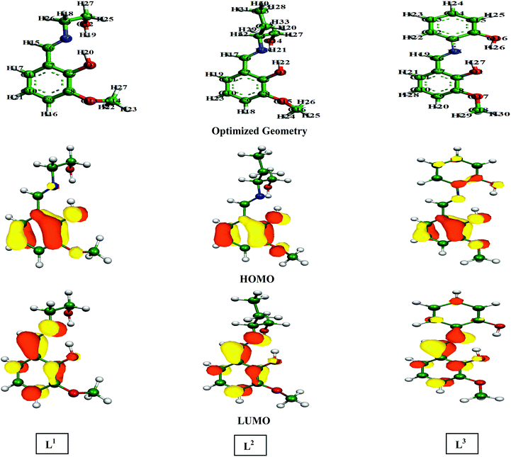 |
| | Fig. 9 Optimized geometry structures, HOMO and LUMO depictions of three Schiff base molecules calculated using the B3LYP method with SV(P), SV/J levels of basis sets. | |
According to FMO theory, the chemical reactivity of the molecules can be analysed by the optimized geometry structure and electron density distribution in the HOMO and LUMO. It was observed from the geometry optimized structure of the inhibitor molecules that all the molecules have a non-planar orientation. However, among the three inhibitors, L1 and L2 are highly non-planar in nature as compared to the L3 inhibitor. Therefore, from the geometry optimized structure of the three studied inhibitors, it is possible to tell that aliphatic chains containing inhibitor molecules cover less surface area than the aromatic moiety containing molecule. In addition to this, if we consider the electron density distribution in the FMOs (i.e.; HOMO and LUMO) of three inhibitors, the electron density is mostly distributed over the azomethine linkage and 2-methoxyphenol segment of the molecule in L1 and L2 inhibitors; the atoms of the aliphatic chains connected to the azomethine linkage are not considerably involved in this distribution. The higher electron density distribution over the azomethine linkage and the 2-methoxyphenol unit is due to the presence of the methoxy (–OCH3 group) and the hydroxyl group (–OH group), which are electron donating groups and the moderately activate electron density distribution of the connected part. However, the electron density distribution in the HOMO and LUMO is distributed widely over the entire molecular skeleton of the L3 inhibitor. This implies that L3 has a higher electron donating and accepting tendency compared to the L1 and L2 inhibitor molecules.
Table 4 contains the calculated quantum chemical parameters of the studied inhibitor molecules. The EHOMO values are remarkably increased in the order of L1 < L2 < L3, which indicates that the electron donating ability followed the order of L3 > L2 > L1. On the other hand, the ELUMO values illustrated that the electron acceptance capability decreases in the sequence of L3 > L2 > L1. Besides the EHOMO and ELUMO values, ΔE values also decrease in the order of L1 > L2 > L3. These results agree well with the results obtained from experimental findings. To further confirm whether our synthesized inhibitor molecules are capable of donating their electrons or not, the fraction of electrons transferred (ΔN) between the inhibitor molecule and the metal surface was calculated. Following Koopmans’ theorem, different intrinsic properties like the ionization potential (I), electron affinity (A), electronegativity (χ), and global hardness (η) of the inhibitors were calculated.66 These parameters are related to each other by the following formula:
| |  | (16) |
| |  | (17) |
From these values, the fraction of electrons transferred (Δ
N) between the inhibitor molecule and the metal surface was calculated by the application of the Pearson method.
67 Having two different electronegative systems in close proximity, the flow of electron takes place from the lower to the higher electronegative site until their chemical potential are equal. The Δ
N value was calculated using the following equation:
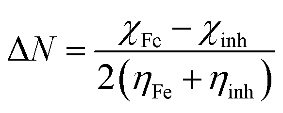
| | 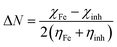 | (18) |
where
χFe and
χinh are the electronegativities, while
ηFe and
ηinh are hardness of the iron and inhibitor molecule, respectively.
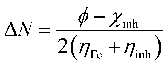
Theoretical values of χFe = 7 eV and ηFe = 0 eV have been incorporated to estimate the ΔN values.68–70 Recently, it was reported that the value of χFe = 7 eV is theoretically not acceptable since electron–electron interactions were not considered; only the free electron gas Fermi energy of iron was considered.12,71,72 For this reason, researchers are using the work function (ϕ) for an appropriate measure of the electronegativity of iron;12,71,72 thus, eqn (18) is rewritten as follows:
| |  | (19) |
In DFT, the
ϕ values for Fe(111), Fe(110) and Fe(100) surfaces are 3.88, 4.82 and 3.91 eV, respectively.
12,71 In the present study, the Fe(110) surface is only considered due to its higher stabilization energy and packed surface. Electron transfer will occur from the inhibitor to the metal surface atom when Δ
N > 0 and
vice versa.
13,14,16 Elnga
et al. reported that there is an increase in the electron donation capability of inhibitor molecules when the Δ
N value is less than 3.6.
73Table 4 shows that all the calculated Δ
N values are positive and less than 3.6, hence, the inhibitor molecules are capable of electron donation to the metallic surface atom. Among the three inhibitor molecules, the L
3 inhibitor has the highest and L
1 has the lowest Δ
N values. It was further confirmed that when the inhibitor molecule is comprised of one aromatic moiety and one small aliphatic chain, there is lower adsorption ability on the mild steel surfaces than that of the inhibitor molecule comprised of two aromatic moieties.
On the other hand, electronegativity is also an important parameter that measures the electron attracting ability of the molecules. The higher the electronegativity, the stronger be the attracting power to accept electrons from the metal surface. Therefore, the inhibitor molecules with higher electronegativity would have strong interactions with the metal surface and obviously higher inhibition efficiency is expected. If we consider the electronegativity values of the studied inhibitors, it can be seen that the electronegativities of the three inhibitors are of the order L3 > L2 > L1. Therefore, from this result, it was confirmed that among the three inhibitor molecules, the L3 inhibitor has the highest electron acceptance capability.
In addition to the abovementioned parameters, global softness (reciprocal of global harness, 1/η) is another parameter of concern, which is also associated with the chemical reactivity of the molecule. According to the Hard and Soft Acids Bases (HSAB) principle, metals are considered as soft acids and inhibitor molecules as soft bases;74 hence, adsorption is preferable for those inhibitor molecules that have higher softness values. The tabulated softness values (Table 4) follow the order of L3 > L2 > L1, which confirms the expected order of inhibition effectiveness. Thus, the experimental findings fully corroborate the theoretical outcomes.
Density functional tight binding calculations
The density functional tight binding (DFTB) method is one of the modern techniques in quantum chemical calculations from which fruitful evaluation of inhibitor–metal interaction can be envisaged. The main advantage of DFTB over the normal DFT method is the inhibitor–metal interaction. Normal DFT calculations only provide molecular behaviours in the solution phase (earlier section). However, how the molecules behave in the presence of the metal surface has not been determined. In this circumstance, DFTB is obviously an advantageous method for evaluating the interactions happening at the inhibitor–metal solution interfaces. It is also noticed that the implementation of the DFTB method in corrosion inhibition chemistry is scanty. Therefore, inhibitor–metal interactions by quantum chemical calculations should be a good addition to the realm of corrosion inhibition chemistry.
Selection of the appropriate iron surface
Before performing the inhibitor–metal interaction by the DFTB+ module (available in Material Studio software version 6.1), it is very necessary to select the appropriate adsorption surface. Herein, a crystal morphology study of the α-Fe crystal was carried out by the morphology module using the equilibrium morphology model. The surface that has the minimum energy can be envisaged from the equilibrium morphology of the crystal.44 If surface free energies for all relevant crystal faces are known, then the morphology of a crystal in equilibrium with its surroundings can be visualized using the Wulff construction plot.75 In the morphology module, the energy of a slab of finite thickness was used for the calculation of surface energy:| | 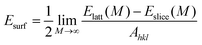 | (20) |
where the energy of a slab, M layers thick, inside the infinite crystal is represented by Elatt(M), the energy of a slab, M layers thick, in a vacuum is denoted by Eslice(M), and the surface area of a plane with Miller indices (hkl) is classified as Ahkl. The factor 1/2 in eqn (20) represents each slab containing two surfaces.
The distance from the origin of the coordinate to the face (hkl) may also be obtained using the following equation:
where
k is a constant and
Dhkl is proportional to the surface energy of the face.
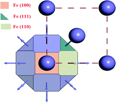
The results obtained from the crystal morphology study of the α-Fe crystal are tabulated in Table 5. The Wulff construction plot for the α-Fe crystal faces are presented in Fig. 10. It is seen that the multiplicities for the Fe(110), Fe(100) and Fe(111) surfaces are 12, 6 and 8, respectively. The calculated surface energies for the abovementioned planes decrease in the following sequence: E(111) > E(100) > E(110). This suggests that among all the surfaces, Fe(110) has the lowest energy surface. The interplanar distance also gradually decreases from Fe(110) to Fe(111). Additionally, the total facet areas (TFA) are ∼63% for Fe(110), ∼24% for Fe(100) and ∼12% for Fe(111) crystal faces. This definitely suggests that the Fe(110) surface has a densely packed surface and also has better stabilization energy. For this reason, the Fe(110) surface was chosen to analyze the adsorption behaviour of the inhibitor molecules on the metallic surfaces.
Table 5 Equilibrium morphology parameters for the α-Fe crystal obtained from the morphology module
|
hkl
|
Multiplicity |
D
hkl
(Å) |
E
surf (kcal mol−1 Å−2) |
TFA (× 108 Å2) |
%TFA |
| Fe(110) |
12 |
2.026 |
9.1596 |
7.987 |
63.31 |
| Fe(100) |
6 |
1.433 |
9.3734 |
3.076 |
24.38 |
| Fe(111) |
8 |
0.827 |
9.8521 |
1.551 |
12.29 |
 |
| | Fig. 10 Wulff construction plot of the α-Fe crystal. | |
Adsorption geometries and energies
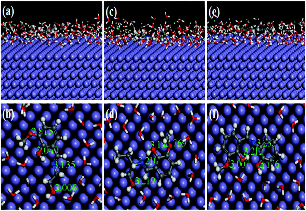
The equilibrium adsorption configurations of the inhibitor molecule on the Fe(110) surfaces obtained from DFTB+ calculations are presented in Fig. 11, where it can be seen that the L3 inhibitor was adsorbed in a flat orientation on the Fe(110) surface, which suggests that all the segments of the inhibitor molecule will take part in the adsorption process. In contrast, in the L1 and L2 inhibitors, only the aromatic part and the hydroxyl group attached to the aliphatic chain take part in the bonding with iron atoms of the Fe(110) surface. The azomethine group and the maximum part of the aliphatic chain do not contribute significantly to the adsorption process. The facial route of the adsorption of L1 and L2 covers less surface area compared to L3, and it is reflected in their inhibition efficiency capabilities. The flat adsorption of the L3 inhibitor is explained in terms of the donor–acceptor type of interaction between the inhibitor molecule and Fe surfaces. It is seen from the molecular structure of the L3 inhibitor that the N and O heteroatom-conjugated π-electrons and aromatic rings are present, which provide enough electrons to the vacant 3d orbital of iron. Electrons coming from the 3d or 4s orbital of iron can also be accommodated in the antibonding orbital of phenyl rings. Coordination, as well as back bonding, facilitated the planar adsorption of L3 inhibitors on the Fe(110) surfaces.
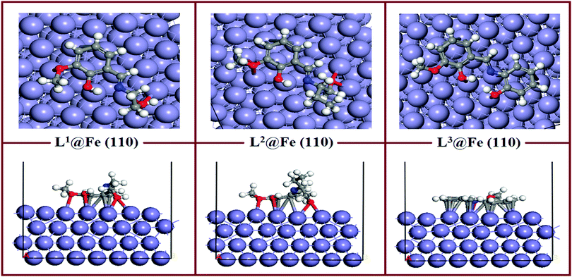 |
| | Fig. 11 Equilibrium adsorption configuration of three Schiff base inhibitors on the Fe(110) surface. Top: Side view, bottom: top view. | |
The calculated adsorption energies and shortest bond distances are given in Table 6. The magnitudes of the adsorption energies for the three adsorption systems are negative, which suggest that all the adsorption processes are energetically favourable. It is also seen that among the three adsorption systems, L3@Fe(110) has the highest Eads value. This suggests that the L3@Fe(110) adsorption system has a more stable and energetically favourable structure than that of the other two adsorption systems. Apart from the Eads values, we have also measured the shortest bond distances between the N/O atom and the closest Fe atom. The shortest O–Fe bond lengths are in the range of 2.731–3.290 Å, which are within the range of 2.5–3.5 Å.76,77 This suggests that chemisorptions occur between the concerned atoms.
Table 6 Shortest bond distance and adsorption energies obtained from DFTB+ calculations
| Systems |
Bond lengths (Å) |
E
ads (kJ mol−1) |
| L1@Fe(110) |
R
O1–Fe
|
2.737 |
−574.17 |
|
R
O12–Fe
|
2.746 |
|
R
O13–Fe
|
2.732 |
|
R
N5–Fe
|
3.919 |
|
|
| L2@Fe(110) |
R
O1–Fe
|
2.747 |
−614.58 |
|
R
O14–Fe
|
2.732 |
|
R
O15–Fe
|
2.731 |
|
R
N5–Fe
|
4.141 |
|
|
| L3@Fe(110) |
R
O1–Fe
|
2.732 |
−655.08 |
|
R
O16–Fe
|
2.734 |
|
R
O17–Fe
|
3.290 |
|
R
N5–Fe
|
2.576 |
However, if we look at the N–Fe bond lengths of the inhibitors (videTable 6) it can be seen that the N–Fe bond lengths are 3.919 Å in L1, 4.141 Å in L2 and 2.576 Å in the L3 inhibitor. The obtained N–Fe bond lengths indicate that the azomethine linkage present in L1 and L2 inhibitors does not take part in the chemisorptions, but the azomethine group in the L3 inhibitor has greater chemisorption ability. Such behaviour can be explained by the chemisorption ability of the hydroxyl group attached to the aliphatic chain of the L1 and L2 inhibitors. Since the oxygen atoms of the hydroxyl groups attached to the aliphatic chains of the L1 and L2 inhibitors have greater adsorption to the Fe surface atom, they will always appear in closer proximity to the Fe surface and create additional strain in the azomethine linkage and the dangling part of the aliphatic chain. Subsequently, these parts of the L1 and L2 inhibitors have less interaction with the Fe surface atom. Thus, it is again established that for the aliphatic chains and aromatic moiety, the aromatic moiety has a greater propensity towards adsorption on the mild steel surfaces.
Charge density difference and population analysis
In order to investigate how the binding of inhibitor molecules affects the electronic distribution at the inhibitor–metal interface, the analysis of the charge density difference (Δρ) is very important. The charge density difference can be computed as follows:44,78| | | Δρ = ρinh@Fe(110) − (ρinh + ρFe(110)) | (22) |
where, ρinh@Fe(110), ρinh and ρFe(110) are the electron densities of the total system, inhibitor molecule and substrate, respectively. The obtained charge density difference for the three adsorption systems are shown in Fig. 12. The charge density difference shows interactions between the inhibitor molecules and iron surface atoms. The loss of electrons is indicated in red, while electron accumulation is indicated in blue. Fig. 12 clearly demonstrates that in L1 and L2 inhibitors, the blue region is mainly localized around the aromatic moiety and hydroxide group attached to the aliphatic chain, whereas in L3 the blue region is distributed throughout the whole molecular section and thus, it is quite obvious that the whole molecule will be responsible for the electron donation. The red region distributed around the surface Fe atom denotes the loss of electrons. If the electron depletion capabilities of the three adsorption systems are compared, it can be seen that L3@Fe(110) has the highest electron depletion capability compared to the other two systems. Thus, the electron depletion and accumulation region reveal that the donor–acceptor interaction is highly facilitated by the L3 inhibitor rather than L1 and L2 inhibitors. The obtained results are accordant with the results obtained from the experiment as well as the normal DFT calculations.
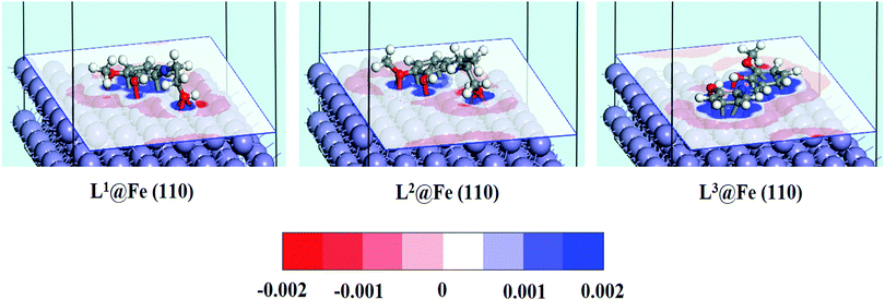 |
| | Fig. 12 Charge density difference for the adsorption systems of Schiff base inhibitors on the Fe(110) surface. The red region indicates the loss of electrons, while electron accumulation is indicated in blue. (Cutoff value of ±0.002 e Å−3). | |
Molecular dynamics simulation
Recently, MD simulation has emerged as an effective tool where interactions between the inhibitor molecule and metal surfaces have been envisaged in a more realistic way.63,64,79 In normal DFT, only molecular behaviours of the inhibitors in the solution phase have been analyzed. However, in the DFTB+ module, the study of metal–inhibitor interactions was carried out in the vacuum phase. Metal–inhibitor interactions in the presence of all concerned species (H2O, H3O+, Cl−) that will actually take part in the corrosion related process are not considered. Thus, to get more insightful results, MD simulations were performed, in which all the entities that will participate in the corrosion related process (such as H2O, H3O+, Cl− and Fe surface) are taken into consideration.
It is well known that the metal surfaces have an affinity for the heteroatoms, π-electrons and aromatic rings of the inhibitor molecules. This needs to be analyzed whether our synthesized inhibitors have the capability to be adsorbed on the metallic surfaces by these sorts of sections or not. In this context, the results obtained from the MD simulation reasonably predict the most preferably adsorbed configuration of inhibitor molecules on the metallic surfaces. It is also worth mentioning that MD simulations reach their equilibrium state when temperature and energy fluctuations have been balanced. From Fig. S18 and S19 (ESI†), it can be seen that at the intermediate step of the simulation, all the dynamic simulations have reached their equilibrium state. The obtained equilibrium adsorption configurations of the inhibitors/Fe(110) system are presented in Fig. 13. All the inhibitor molecules tend to adsorb in a more or less planar orientation on the Fe(110) surface. These parallel orientations maximize the contact between the inhibitor molecule and the surface of the Fe atom; therefore, the dissolution of the Fe surface resulting from aggressive acidic attacks is minimized. As such, superior inhibition effectiveness was expected and obtained accordingly. On closer inspection, it was also seen that among the three studied inhibitors, L3 adsorbed in a nearly planar orientation and thus covered a higher surface area in comparison to the other two inhibitor molecules. Higher surface area coverage by the L3 inhibitor is one of the prime reasons for its higher inhibition efficiency. Furthermore, in order to analyze whether heteroatoms present in the molecular skeleton have participated in the bonding, we measured the shortest bond distances among the heteroatoms of the inhibitor and closest Fe atom. It can be seen from Fig. 13 that all the bond distances are within the range of 2.5–3.5 Å. This indicates that chemical bonds were formed between the heteroatoms of the inhibitor molecule and Fe atoms.76,77 Moreover, from the interaction and binding energy between the inhibitor molecules and the Fe(110) surface, it is also possible to analyze the adsorption ability of the studied inhibitors. From Table 7, the obtained interaction energies for adsorption systems at 300 K are −556.37, −591.57 and −654.35 kJ mol−1, respectively. These high absolute negative values of interaction energy indicate that a strong interaction has occurred between the inhibitor molecule and the concerned metallic surface. The obtained interaction energy value also reveals that the L3 inhibitor adsorbed more spontaneously than L2 and L1 inhibitors. In addition to this, the binding ability is also a very good measure of the adsorption capability of the molecules. The adsorption capability of the inhibitor molecules increases with increasing binding energy. Binding energy values reflected from Table 7 follow the order: L3 > L2 > L1. This further reflects that the L3 inhibitor has higher binding ability than that of the L2 inhibitor and the L1 inhibitor has the least adsorption ability. Hence, it is concluded that MD simulated results concurred well with quantum chemical calculation outcomes and also the results obtained from experimentation.
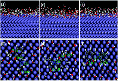 |
| | Fig. 13 Equilibrium adsorption configuration of three Schiff base inhibitors [L1 (a and b), L2 (c and d) and L3 (e and f)] on the Fe(110) plane obtained by MD simulation. Top: Side view, bottom: top view. | |
Table 7 Interaction energies and binding energy values between the inhibitors and the Fe(110) plane
| Systems |
E
interaction (kJ mol−1) |
E
binding (kJ mol−1) |
| Fe(110) + L1 |
−556.37 |
556.37 |
| Fe(110) + L2 |
−591.57 |
591.57 |
| Fe(110) + L3 |
−654.35 |
654.35 |
Conclusion
The adsorption behaviours of small aliphatic chains, branched aliphatic chains and aromatic substituents containing corrosion inhibitors on mild steel surfaces have been studied by a complete experimental and theoretical investigation. The outcome obtained from the experimental studies clearly manifests that the effects exerted by the heteroatoms, π electrons of the aromatic ring and, most importantly, the stereochemical configuration of the molecules play a dominant role in adsorption ability of the inhibitor molecules on the mild steel surfaces. The results obtained from the electrochemical measurement and gravimetric analysis revealed that at the concentration of 5 mM, the maximum inhibition efficiency reached 94.4%, 95.9% and 97.1% for L1, L2 and L3, respectively. It clearly indicates that the corrosion inhibition efficiency follows the order: L3 > L2 > L1. This result exemplifies that among the three structurally similar inhibitor molecules, one having a small aliphatic chain in the organic scaffold provides lower adsorption ability compared to another having an aromatic moiety in the structural unit of the inhibitor molecule. The obtained gravimetric results also manifest that all the inhibitor molecules actively show their inhibition capability up to an immersion time of 96 h. The adsorption of the inhibitor molecules on the mild steel surface follows the Langmuir adsorption isotherm and the obtained ΔG0ads values reveal that all the inhibitor molecules can be broadly classified as mixed-type inhibitors, where the chemisorption property is predominant over the physical adsorption. The adsorption of the inhibitors on the mild steel surface was also established by FESEM, EDX and AFM analysis. Contact angle measurements also demonstrated that the presence of inhibitor molecules in the aggressive acidic solution makes the hydrophilic surface mostly hydrophobic in nature. Quantum chemical calculations using DFT were employed to analyze the effectiveness of the inhibitor molecules. The obtained quantum chemical parameters (such as EHOMO, ELUMO, ΔE, χ, η, S and ΔN), and electron density distributions in the FMOs demonstrated that all the inhibitor molecules are capable of adsorption and their strength of adsorption decreased in the order of L3 > L2 > L1. Most importantly, the DFTB study manifests that the azomethine linkage and the dangling part of the aliphatic chain present in the molecular skeleton of L1 and L2 inhibitors do not participate significantly in the D–A type of interaction phenomena with the mild steel surface, whereas the L3 inhibitor as a whole participated in bonding. With the aim to obtain additional information on the adsorption behaviour of inhibitor molecules on the mild steel surface, MD simulations in the presence of all concerned species (Fe surface, H2O, H3O+, Cl−) have been carried out. The obtained results revealed that all the inhibitor molecules were adsorbed more or less parallel in orientation with respect to the Fe(110) surface. In addition to this, the measured bond distances among the heteroatoms of inhibitor molecules and the closest Fe atom also demonstrated that chemical bonds have been formed between the two interacting species. The obtained binding energy and interaction energy values also follow the order of L3 > L2 > L1, which is also in accordance with quantum chemical calculation outcomes and experimentally obtained results.
In summary, both experimental and theoretical results support that among the small aliphatic chains, the branched aliphatic chain and the aromatic-containing moiety, the aromatic containing moiety has a greater propensity towards adsorption on the mild steel surfaces and therefore, the greatest inhibition efficiency was exhibited by the L3 inhibitor molecule. The experimental analysis followed by quantum chemical calculation and finally molecular dynamics simulations provide absolute clarification of extremely concerning issues in the realm of corrosion inhibition.
Conflicts of interest
There are no conflicts of interest to declare.
Acknowledgements
Department of Science and Technology (DST), Govt. of India sponsored Project (vide ref. no. DST/TSG/WM/2015/459 and project no. GAP-211712) is hereby acknowledged. SKS would like to acknowledge the DST, New Delhi, India for his DST INSPIRE Fellowship. Authors are also thankful to Ms Suparna Paul, CSIR-CMERI and Mr Samuzal Bhuyan, Sikkim University for their support.
Notes and references
- D. de la Fuente, I. Diaz, J. Simancas, B. Chico and M. Morcillo, Corros. Sci., 2011, 53, 604–617 CrossRef.
- S. B. Ulaeto, U. J. Ekpe, M. A. Chidiebere and E. E. Oguzie, Int. J. Mater. Chem., 2012, 2, 158–164 Search PubMed.
- M. A. Hegazy, A. S. El-Tabei, A. H. Bedair and M. A. Sadeq, RSC Adv., 2015, 5, 64633–64650 RSC.
- I. Ahamad, R. Prasad and M. A. Quraishi, Corros. Sci., 2010, 52, 3033–3041 CrossRef.
- M. Gopiraman, N. Selvakumaran, D. Kesavan, I. S. Kim and R. Karvembu, Ind. Eng. Chem. Res., 2012, 51, 7910–7922 CrossRef.
- U. F. Ekanem, S. A. Umoren, I. I. Udousoro and A. P. Udoh, J. Mater. Sci., 2010, 45, 5558–5566 CrossRef.
- M. Jeeva, G. V. Prabhu, M. S. Boobalan and C. M. Rajesh, J. Phys. Chem. C, 2015, 119, 22025–22043 CrossRef.
- K. F. Khaled, Int. J. Electrochem. Sci., 2008, 3, 462–475 Search PubMed.
- M. Lebrini, A. Lagrenee, A. Traisnel, L. Gengembre, H. Vezin and F. Bentiss, Appl. Surf. Sci., 2007, 253, 9267–9276 CrossRef.
- D. Guzman-Lucero, O. Olivares-Xometl, R. Martinez-Palou, N. V. Likhanova, M. A. Dominguez-Aguilar and V. Garibay-Febles, Ind. Eng. Chem. Res., 2011, 50, 7129–7140 CrossRef.
- D. K. Yadav and M. A. Quraishi, Ind. Eng. Chem. Res., 2012, 51, 8194–8210 CrossRef.
- S. K. Saha, A. Dutta, P. Ghosh, D. Sukul and P. Banerjee, Phys. Chem. Chem. Phys., 2015, 17, 5679–5690 RSC.
- S. K. Saha, P. Ghosh, A. Hens, N. C. Murmu and P. Banerjee, Phys. E, 2015, 66, 332–341 CrossRef.
- S. K. Saha, A. Dutta, P. Ghosh, D. Sukul and P. Banerjee, Phys. Chem. Chem. Phys., 2016, 18, 17898–17911 RSC.
- S. K. Saha and P. Banerjee, RSC Adv., 2015, 5, 71120–71130 RSC.
- A. Dutta, S. K. Saha, P. Banerjee and D. Sukul, Corros. Sci., 2015, 98, 541–550 CrossRef.
- G. Achary, H. P. Sachin, Y. A. Naik and T. V. Venkatesha, Mater. Chem. Phys., 2008, 107, 44–50 CrossRef.
- L. O. Olasunkanmi, I. B. Obot, M. M. Kabanda and E. E. Ebenso, J. Phys. Chem. C, 2015, 119, 16004–16019 CrossRef.
- H. D. Leçe, K. C. Emregül and O. Atakol, Corros. Sci., 2008, 50, 1460–1468 CrossRef.
- S. Issaadi, T. Douadi, A. Zouaoui, S. Chafaa, M. A. Khan and G. Bouet, Corros. Sci., 2011, 53, 1484–1488 CrossRef.
- K. R. Ansari and M. A. Quraishi, Corros. Sci., 2014, 79, 5–15 CrossRef.
- Y. Zhou, S. Xu, L. Guo, S. Zhang, H. Lu, Y. Gong and F. Gao, RSC Adv., 2015, 5, 14804–14813 RSC.
- S. Shahabi, P. Norouzi and M. R. Ganjali, Int. J. Electrochem. Sci., 2015, 10, 2646–2662 Search PubMed.
-
(a) P. Ghosh and P. Banerjee, Phys. Chem. Chem. Phys., 2016, 18, 22805–22815 RSC;
(b) P. Ghosh, A. R. Chowdhury, S. K. Saha, M. Ghosh, M. Pal, N. C. Murmu and P. Banerjee, Inorg. Chim. Acta, 2015, 429, 99–108 CrossRef.
- S. K. Saha, A. Hens, N. C. Murmu and P. Banerjee, J. Mol. Liq., 2016, 215, 486–495 CrossRef.
- E. E. Oguzie, C. B. Adindu, C. K. Enenebeaku, C. E. Ogukwe, M. A. Chidiebere and K. L. Oguzie, J. Phys. Chem. C, 2012, 116, 13603–13615 CrossRef.
- S. U. Ofoegbu, T. L. P. Galvao, J. R. B. Gomes, J. Tedim, H. I. S. Nogueira, M. G. S. Ferreira and M. L. Zheludkevicha, Phys. Chem. Chem. Phys., 2017, 19, 6113–6129 RSC.
-
(a) L. F. L. Oliveira, N. Tarrat, J. Cuny, J. Morillo, D. Lemoine, F. Spiegelman and M. Rapacioli, J. Phys. Chem. A, 2016, 120, 8469–8483 CrossRef PubMed;
(b) M. Elstner, D. Porezag, G. Jungnickel, J. Elsner, M. Haugk, T. Frauenheim, S. Suhai and G. Seifert, Phys. Rev. B: Condens. Matter Mater. Phys., 1998, 58, 7260–7268 CrossRef.
- I. Kaya, S. Culhaoglu and D. Senol, Chin. J. Polym. Sci., 2007, 25, 461–472 CrossRef.
-
J. Coates, Interpretation of Infrared Spectra, A Practical Approach, John Wiley & Sons Ltd, Chichester, 2000 Search PubMed.
-
B. Stuart, Infrared Spectroscopy: Fundamentals and Applications, Wiley, 2004 Search PubMed.
-
F. Neese, An Ab initio, DFT and Semiempirical SCF-MO Package, Version 2.7.0, Max Planck Institute for Bioinorganic Chemistry, Mulheim an der Ruhr, Germany, 2012 Search PubMed.
- D. A. Becke, J. Chem. Phys., 1986, 84, 4524–4529 CrossRef.
- D. A. Becke, J. Chem. Phys., 1993, 98, 5648–5652 CrossRef.
- C. Lee, W. Yang and R. G. Parr, Development of the Colle-Salvetti correlation-energy formula into a functional of the electron density, Phys. Rev. B: Condens. Matter Mater. Phys., 1988, 37, 785–789 CrossRef.
- P. Banerjee, A. Company, T. Weyhermuller, E. Bill and C. R. Hess, Inorg. Chem., 2009, 48, 2944–2955 CrossRef PubMed.
- P. Banerjee, S. Sproules, T. Weyhermuller, S. D. George and K. Wieghardt, Inorg. Chem., 2009, 48, 5829–5847 CrossRef PubMed.
- A. Schafer, C. Huber and R. Ahlrichs, J. Chem. Phys., 1994, 100, 5829–5835 CrossRef.
- A. Schafer, H. Horn and R. Ahlrichs, J. Chem. Phys., 1992, 97, 2571–2577 CrossRef.
- M. Elstner and G. Seifert, Philos. Trans. R. Soc., A, 2014, 372, 20120483 CrossRef PubMed.
- P. Koskinen and V. Mäkinen, Comput. Mater. Sci., 2009, 47, 237–253 CrossRef.
- A. F. Oliveira, G. Seifert, T. Heine and H. A. Duarte, J. Braz. Chem. Soc., 2009, 20, 1193–1205 CrossRef.
-
Materials Studio 6.1 Manual, Accelrys, Inc., San Diego, CA, 2007 Search PubMed.
- L. Guo, C. Qi, X. Zheng, R. Zhang, X. Shen and S. Kaya, RSC Adv., 2017, 7, 29042–29050 RSC.
- G. Kresse and J. Furthmuller, Phys. Rev. B: Condens.
Matter Mater. Phys., 1996, 54, 11169–11186 CrossRef.
- T. Chakraborty, A. Hens, S. Kulashresth, N. C. Murmu and P. Banerjee, Phys. E, 2015, 69, 371–377 CrossRef.
- H. Sun, J. Phys. Chem. B, 1998, 102, 7338–7364 CrossRef.
- S. W. Bunte and H. Sun, J. Phys. Chem. B, 2000, 104, 2477–2489 CrossRef.
- E. S. Ferreira, C. Giacomelli, F. C. Giacomelli and A. Spinelli, Mater. Chem. Phys., 2004, 83, 129–134 CrossRef.
- M. A. Hegazy, Corros. Sci., 2009, 51, 2610–2618 CrossRef.
- R. Solmaz, Corros. Sci., 2010, 52, 3321–3330 CrossRef.
- R. Solmaza, G. Kardas, M. Culha, B. Yazıcı and M. Erbil, Electrochim. Acta, 2008, 53, 5941–5952 CrossRef.
- X. Wu, H. Ma, S. Chen, Z. Xu and A. Sui, J. Electrochem. Soc., 1999, 146, 1847–1853 CrossRef.
- T. Wang, L. Tan, C. Ding, M. Wang, J. Xu and J. Fu, J. Mater. Chem. A, 2017, 5, 1756–1768 RSC.
- E. E. Oguzie, Y. Li and F. H. Wang, Electrochim. Acta, 2007, 52, 6988–6996 CrossRef.
- M. A. Ameer, E. Khamis and G. Al-Senani, J. Appl. Electrochem., 2002, 32, 149–156 CrossRef.
- P. Roy and D. Sukul, RSC Adv., 2015, 5, 1359–1365 RSC.
- S. Issaadi, T. Douadi, A. Zouaoui, S. Chafaa, M. A. Khan and G. Bouet, Corros. Sci., 2011, 53, 1484–1488 CrossRef.
- R. Solmaz, Corros. Sci., 2014, 79, 169–176 CrossRef.
- R. Solmaz, Corros. Sci., 2014, 81, 75–84 CrossRef.
- F. S. de Souza, R. S. Gonçalves and A. Spinelli, J. Braz. Chem. Soc., 2014, 25, 81–90 Search PubMed.
- I. B. Obot, Z. M. Gasem and S. A. Umoren, Int. J. Electrochem. Sci., 2014, 9, 510–522 Search PubMed.
- C. Verma, L. O. Olasunkanmi, E. E. Ebenso, M. A. Quraishi and I. B. Obot, J. Phys. Chem. C, 2016, 120, 11598–11611 CrossRef.
- Y. Qiang, S. Zhang, L. Guo, X. Zheng, B. Xiang and S. Chen, Corros. Sci., 2017, 119, 68–78 CrossRef.
- K. Rengaraj, B. Sivasankar, M. Anbu and M. Palanichamy, J. Chem. Sci., 1991, 103, 707–713 Search PubMed.
- I. Lukovits, E. Kalman and F. Zucchi, Corrosion, 2001, 57, 3–8 CrossRef.
- S. Martinez, Mater. Chem. Phys., 2003, 77, 97–102 CrossRef.
- A. Y. Musa, A. A. H. Kadhum, A. B. Mohamad and M. S. Takriff, Mater. Chem. Phys., 2011, 129, 660–665 CrossRef.
- H. Shokry, J. Mol. Struct., 2014, 1060, 80–87 CrossRef.
- A. Y. Musa, R. T. T. Jalgham and A. B. Mohamad, Corros. Sci., 2012, 56, 176–183 CrossRef.
- A. Kokalj, Chem. Phys., 2012, 393, 1–12 CrossRef.
- I. B. Obot, D. D. Macdonald and Z. M. Gasem, Corros. Sci., 2015, 99, 1–30 CrossRef.
- M. K. Awad, M. R. Mustafa and M. M. A. Elnga, THEOCHEM, 2010, 959, 66–74 CrossRef.
- I. B. Obot and Z. M. Gasem, Corros. Sci., 2014, 83, 359–366 CrossRef.
- D. Winn and M. F. Doherty, AIChE J., 2000, 46, 1348–1367 CrossRef.
- W. Y. Shi, C. Ding, J. L. Yan, X. Y. Han, Z. M. Lv, W. Lei, M. Z. Xia and F. Y. Wang, Desalination, 2012, 291, 8–14 CrossRef.
- J. P. Zeng, J. Y. Zhang and X. D. Gong, Comput. Theor. Chem., 2011, 963, 110–114 CrossRef.
- T. A. Baker, C. M. Friend and E. Kaxiras, J. Am. Chem. Soc., 2008, 130, 3720–3721 CrossRef PubMed.
- P. Singh, E. E. Ebenso, L. O. Olasunkanmi, I. B. Obot and M. A. Quraishi, J. Phys. Chem. C, 2016, 120, 3408–3419 CrossRef.
Footnote |
| † Electronic supplementary information (ESI) available: FTIR, ESI-MS, 1H-NMR, 13C-NMR, potentiodynamics polarization curves, Nyquist plots, weight loss measurements, EDX, temperature and energy fluctuation obtained from MD simulation. See DOI: 10.1039/c8qm00162f |
|
| This journal is © the Partner Organisations 2018 |
Click here to see how this site uses Cookies. View our privacy policy here. 
 ab and
Priyabrata
Banerjee
ab and
Priyabrata
Banerjee