
 Open Access Article
 This Open Access Article is licensed under a
 Creative Commons Attribution 3.0 Unported Licence
The impact of tilt grain boundaries on the thermal transport in perovskite SrTiO3 layered nanostructures. A computational study†
Stephen R.
Yeandel
 ab,
Marco
Molinari
ac and
Stephen C.
Parker
*a
ab,
Marco
Molinari
ac and
Stephen C.
Parker
*a
aDepartment of Chemistry, University of Bath, Claverton Down, Bath, BA2 7AY, UK. E-mail: s.c.parker@bath.ac.uk; m.molinari@hud.ac.uk
bDepartment of Chemistry, Loughborough University, Epinal Way, Loughborough, LE11 3TU, UK
cDepartment of Chemistry, University of Huddersfield, Queensgate, Huddersfield, HD1 3DH, UK
First published on 19th July 2018
Abstract
Thermal management at solid interfaces presents a technological challenge for modern thermoelectric power generation. Here, we define a computational protocol to identify nanoscale structural features that can facilitate thermal transport in technologically important nanostructured materials. We consider the highly promising thermoelectric material, SrTiO3, where tilt grain boundaries lower thermal conductivity. The magnitude of the reduction is shown to depend on compositional and structural arrangements at the solid interface. Quantitative analysis indicates that layered nanostructures less than 10 nm will be required to significantly reduce the thermal conductivity below the bulk value, and it will be virtually independent of temperature for films less than 2 nm depending on the orientation with a reduction of thermal transport up to 75%. At the nanoscale, the vibrational response of nanostructures shows concerted vibrations between the grain boundary and inter-boundary regions. As the grain boundary acts markedly as a phonon quencher, we predict that any manipulation of nanostructures to further reduce thermal conductivity will be more beneficial if applied to the inter-boundary region. Our findings may be applied more widely to benefit other technological applications where efficient thermal transport is important.
1. Introduction
The topic of thermal transport at nanoscale structural features is enjoying great interest.1–7 In thermoelectric (TE) technology, an alternative sustainable route for energy harvesting,8 thermoelectric materials directly convert waste heat into usable electricity, and any structural feature at the nanoscale has a key role in modifying materials’ performance in terms of thermal transport.The conversion efficiency of a TE material is elegantly defined by the dimensionless figure of merit ZT = (TσS2)/(κe + κl), which arises from an intricate balance between the Seebeck coefficient or thermopower, S, the electrical conductivity, σ, the electronic (κe) and lattice (κl) contributions to the thermal conductivity and temperature, T.
In these materials there are two main strategies to improve efficiency. One is to maximize the electrical conductivity and the Seebeck coefficient through band engineering,8–12 and the other is to reduce the lattice thermal conductivity (κl) by nanostructuring or phonon engineering.1–7,13
Nanostructuring introduces structural features at the nanoscale and for thermoelectric materials based on oxides, this is the currently preferred route for lowering their high thermal conductivity. One of the most promising oxides for the n-type material of a thermoelectric device is SrTiO3. Its structural design and engineering has been under the research spotlight in the last decade, with research proposing assemblages and thin films to lower its thermal conductivity via enhanced phonon scattering and confinement in sufficiently small systems.3,14–18
The most basic form of nanostructuring is the introduction of interfaces19–26 as they are present in polycrystalline systems, as well as in thin and layered nanostructures. However, a greater control on the distribution of these interfaces will generate nanostructured materials with tailor-made properties.27–33 Generally in polycrystalline materials this control is lost as the grains adopt a random distribution after sintering. Synthetic experimental methodology with high control of shape and morphology, such as atomic layer deposition,34–36 could radically change this, although due to the high cost of implementation, it would be preferential to avoid trial and error experimentation, and instead generate the final product with specific orientated interfaces. Control of the interface morphology and orientation will lead to more efficient thermoelectric materials, particularly if experiment could be guided to synthesise the optimal microstructure.3,13,14,37–40 To this end computational techniques can provide an effective strategy for evaluating the contribution of individual interfaces to phonon scattering, and for ranking their effect on thermal conductivity. This is a valuable contribution as it is extremely challenging to measure thermal conductivity of films accurately, particularly when the sample thickness is as small as a few nanometers.41–43
The current work addresses these challenges and aims to demonstrate a predictive framework based on molecular and lattice dynamics calculations of the thermal transport at interfaces. We examine the vibrational response of three layered nanostructures of SrTiO3, and analyse its effect on the out-of-plane and the in-plane thermal conductivity. Finally, we discuss the implication of this relationship in predicting efficient reduction in thermal conductivity and thus optimal nanostructures.
2. Computational methods
2.1 Layered nanostructure models
Layered nanostructures containing three different interfaces, i.e. Σ3{111}/[![[1 with combining macron]](https://www.rsc.org/images/entities/char_0031_0304.gif) 10], Σ3{112}/[10] and Σ5{310}/[001] tilt grain boundaries (Fig. 1), were constructed using the methodology outlined in Williams et al.44 and the METADISE code.45 These interfaces are chosen as they represent three very distinct structures found experimentally.46 Strontium titanate is known to have space charge layers at grain boundaries that can reach a thickness of tens of nanometres.47–49 In this space charge layer, the crystal is defective. However, as our investigation is concerned with the determination of the intrinsic contribution of structural features, independently on other defects, we omit these additional defects. This is to avoid an extra level of complexity that we will not be able to separate easily, i.e. the contribution of point defect (oxygen vacancies) from the contribution of extended defects (grain boundaries). Finally our configurations can be thought as air sintered samples where the amount of oxygen vacancies will decrease dramatically.50,51
10], Σ3{112}/[10] and Σ5{310}/[001] tilt grain boundaries (Fig. 1), were constructed using the methodology outlined in Williams et al.44 and the METADISE code.45 These interfaces are chosen as they represent three very distinct structures found experimentally.46 Strontium titanate is known to have space charge layers at grain boundaries that can reach a thickness of tens of nanometres.47–49 In this space charge layer, the crystal is defective. However, as our investigation is concerned with the determination of the intrinsic contribution of structural features, independently on other defects, we omit these additional defects. This is to avoid an extra level of complexity that we will not be able to separate easily, i.e. the contribution of point defect (oxygen vacancies) from the contribution of extended defects (grain boundaries). Finally our configurations can be thought as air sintered samples where the amount of oxygen vacancies will decrease dramatically.50,51
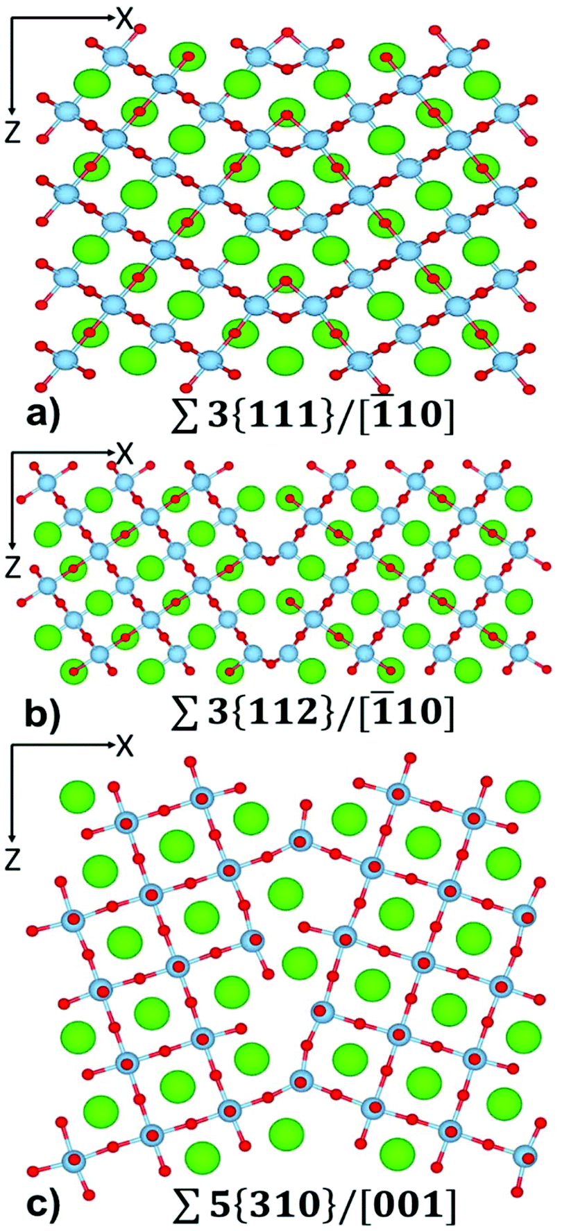 | ||
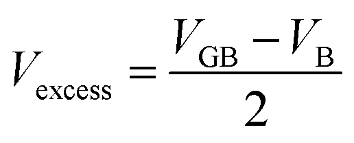
| Fig. 1 The atom-level structure of (a) Σ3{111}/[10], (b) Σ3{112}/[10] and (c) Σ5{310}/[001] tilt grain boundary in SrTiO3. Sr = green, Ti = pale blue, O = red. | ||
All simulated systems (i.e. layered nanostructures) contain two identical grain boundaries with the X direction perpendicular to the YZ boundary plane. To evaluate the role of the inter-boundary distance (i.e. the distance between two tilt grain boundary) on thermal transport, we constructed layered nanostructure configurations with grain boundaries far from each other (∼10 nm referred to as 10 nm-GB), and close to each other (∼2 nm referred to as 2 nm-GB). This provides information on the extent that the inter-boundary region limits the allowed phonon wavelengths.
The lattice parameters of all simulated layered nanostructures are provided in Table S1.† The a, b and c cell dimensions correspond to the direction x, y and z respectively. For all calculations, we used the potential model developed by Teter,52 which has been validated extensively for the assemblage of SrTiO3 nanocubes14 and for other perovskite oxides.53–55
2.2 Thermal conductivity and vibrational response
Molecular dynamics calculations were performed using the LAMMPS code.56 We use 3D periodic boundary conditions, thus the unit cell is surrounded by identical images in all directions. Each layered nanostructure was annealed initially at high temperature (1500 K) to check structural stability, then thermally equilibrated at each temperature (500 K–1300 K) for 50 ps with a timestep of 1 fs using an NPT anisotropic ensemble. The ensemble employed a Nosé–Hoover thermostat and barostat. The lattice vectors were averaged every 10 fs. The simulation was deemed to converge when the energy fluctuations were consistently less than 0.1% of the average energy value and the volume fluctuations were less than 0.5% of the average volume. The averaged vectors were then imposed on the simulation cell for calculation of thermal conductivity. The lattice thermal conductivity for each layered nanostructure at five different temperatures was calculated using the Green–Kubo method.57,58 A brief explanation of the methodology used is provided in ESI section S1.† The heat-flux was collected sequentially for 20 ns, sampled every 10 fs, the heat-flux was numerically autocorrelated and integrated to give an integral as a function of time, which is then averaged over a portion of the integral itself to reduce the noise in the thermal conductivity.14,59 The value of thermal conductivity was averaged over a region of ‘neck regime’.14,60 Convergence tests for the dependence of the thermal conductivity on the size of the unit cells are presented in ESI section S1.† Depending on the direction of the heat flux, whether perpendicular (i.e. the X direction of our unit cell) or parallel (i.e. the Y and Z directions of our unit cell) to the grain boundary, one can calculate the out-of-plane and the in-plane contribution to the thermal conductivity, respectively. Finally, the Fourier transform of the heat-flux autocorrelation function yields the spectrum of the heat-flux autocorrelation function (HFACF),60 which relates to the optical vibrational modes capable of interacting with acoustic vibrational modes and thus the heat-flux of the system.61,62 In this manner these optical vibrational modes are routes for phonon–phonon Umklapp processes to dissipate heat.632.3 Phonon density of states
To aid in the interpretation of HFACF, we performed lattice dynamics calculations on model systems (i.e. representing the layered nanostructures) using the PHONOPY code64,65 and the METADISE code.45 These models referred to as lattice dynamics grain boundaries (LD-GB) are equivalent to the 2 nm-GB interacting systems, with the same inter-boundary distance but reduced size of the YZ boundary plane. This is necessary to reduce the computational effort for this type of calculation. LD calculations provide the phonon density of states (PDOS) and aid the identification of species within the lattice which are involved in the scattering processes contributing to lowering of the thermal conductivity.62 The PDOS contain only optical phonon frequencies at the Γ-point and can be compared to the HFACF spectra upon analysis (section SI1†).14 The peaks, which appear in both PDOS and HFACF are also IR active modes as there will be an accompanying change in dipole with their underlying vibrational motion. For each peak of the PDOS and HFACF spectra, we have provided a detailed analysis of the vibrational mode involved, separating the contributions from the grain boundary (GB) and the inter-boundary (IB) regions. This analysis provides a quantitative evaluation of the predominant contribution to the thermal conductivity arising from the grain boundary and the inter-boundary regions. Full details of our analysis are found in ESI (section S1†).2.4 Formation energies of grain boundaries
Eqn (1) was used to calculate the formation energy of all grain boundary configurations. The formation energy, Ef, is obtained by subtracting the energy of a bulk system (Eb) with the same number of atoms from the energy of each grain boundary system (Egb), and dividing by the surface area (A, i.e. the YZ boundary plane) occupied by each grain boundary (i.e. there are two grain boundaries in each configuration).44,66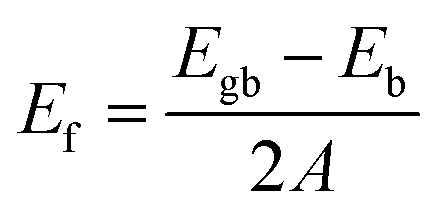 | (1) |
The energies for the 2 nm-GB and 10 nm-GB are obtained by averaging the configurational energy of grain boundaries over the molecular dynamics calculations (section 2.2), whereas the lattice energies for the LD-GB were obtained using lattice dynamics calculations as implemented in the METADISE code.45 To note is that whereas lattice dynamics does not account for temperature effects, molecular dynamics does.
3. Results and discussion
3.1 Characterization of grain boundary structures and energetics
Each layered nanostructure is characterized by interfaces with specific orientation. These are tilt grain boundaries. Here, we provide a brief characterization of their structure compared to experimental data.The structure of Σ3{111}/[10] (Fig. 1(a)) is known from HRTEM studies.67 Density Functional Theory (DFT) calculations have shown that the Ti–O bonding network is partially preserved across the boundary, indicating the possibility of lowering the thermal conductivity whilst retaining electrical conductivity.68 The Σ3{111}/[10] boundary is made of face sharing TiO6 octahedra. All Sr species at the boundary remain in a 12-fold coordination environment with one of the Sr–O distances elongated at 3.0 Å compared with bulk distance of 2.8 Å. Sr species are also at the centre of a HCP packed polyhedra rather than of a FCC packed polyhedra as found in bulk SrTiO3.
Two structures have been observed for the Σ3{112}/[10] grain boundary using HRTEM;69 a mirror symmetric structure and a mirror-glide symmetric structure. We focussed on the mirror-glide structure (Fig. 1(b)) as it is stable, and displays no reconstruction during the annealing at temperatures greater than 1500 K. Furthermore, the structures were indistinguishable in terms of energy using DFT calculations.70 The structure of the mirror-glide symmetric Σ3{112}/[10] boundary has a larger range of local Sr and Ti coordination environments. There are edge sharing octahedral TiO6, square-based pyramidal TiO5, Sr cuboctahedron environments (Sr–O distances: 10 at 2.8 Å and 2 at 3.0 Å) and 10-fold coordinated Sr environments (Sr–O distances: 8 at 2.8 Å and 2 at 3.3 Å).
Combined experimental work and first principles calculations found that the structure of Σ5{310}/[001] is asymmetric.71 This boundary has been shown to undergo temperature dependent faceting using high-resolution electron microscopy,72 with many possible structures with similar energy identified via atomistic simulations.73 This complexity results in a large number of possible configurations for this boundary. The Σ5{310}/[001] grain boundary chosen in our study (Fig. 1(c)) shows a large number of Ti environments at the boundary, including corner sharing trigonal bipyramidal TiO5, squared pyramidal TiO5, and octahedral TiO6, with many of these environments having dangling O species. There are also many symmetrically inequivalent Sr species at the boundary, including 9-fold coordinated Sr (all Sr–O distances up to 2.9 Å), 11 and 12-fold coordinated (Sr–O distances up to 3.0 Å), and 12-fold coordinated (Sr–O distances up to 3.4 Å).
Till now, we have described the structures of the grain boundaries. We can also define the structural complexity of the grain boundaries via quantitative analysis of their structures.71,74,75 We define structural complexity as (1) distance between the grain boundaries (i.e. the interaction between the grain boundaries), (2) density of the grain boundary, (3) volume excess (i.e. the number of SrTiO3 unit missing at the grain boundary), and (4) dangling bonds per unit area.
Firstly, the grain boundaries are 2 nm or 10 nm apart and these represent the inter-boundary distances as described in section 2.1.
Secondly, we have calculated the density, (d) expressed as NSrTiO3/nm3, of the different 2 nm-GB and 10 nm-GB configurations simulated using molecular dynamics. For simplicity the density values have been scaled considering a density of 1 NSrTiO3/nm3 for stoichiometric bulk SrTiO3. Table 1 reports the values obtained. For systems where the grain boundaries are 10 nm apart, the density of Σ3{112}/[10] and Σ5{310}/[001] are closer to each other and smaller than the density of Σ3{111}/[10]. For the systems where the distance between the boundary is 2 nm apart, the density values of Σ3{111}/[10] and Σ3{112}/[10] are now similar and higher than the density of Σ5{310}/[001].
| Grain boundary configuration | Density (NSrTiO3/nm3) |
|---|---|
| Stoichiometric bulk SrTiO3 | 1.000 |
| 10 nm-GB Σ3{111}/[10] |
0.997 |
| 10 nm-GB Σ3{112}/[10] |
0.994 |
| 10 nm-GB Σ5{310}/[001] | 0.992 |
| 2 nm-GB Σ3{111}/[10] |
0.979 |
| 2 nm-GB Σ3{112}/[10] |
0.971 |
| 2 nm-GB Σ5{310}/[001] | 0.937 |
Thirdly, we have defined the number of SrTiO3 units missing at the grain boundary. We defined the excess volume, Vexcess, (eqn (2)) as the difference between the volume of the grain boundary structure, VGB, and the volume of stoichiometric bulk SrTiO3, VB; both quantities have an equivalent number of SrTiO3 units and we need to account for a factor of 2 as there are two grain boundaries in each configuration.
 | (2) |
V
excess can be divided by the volume of one unit of stoichiometric bulk SrTiO3 and by the surface area of the grain boundary plane (SGB) to provide the number of SrTiO3 units per nm2 (NSrTiO3) that are missing at the grain boundary (eqn (3)).
 | (3) |
We have calculated NSrTiO3 for all layered nanostructures simulated using lattice and molecular (at 500 K) dynamics (Table 2). Σ3{111}/[10] is the most dense boundary followed by Σ3{112}/[10] and Σ5{310}/[001] compared to stoichiometric bulk SrTiO3, as it has the smallest values of NSrTiO3.
| Grain boundary | N SrTiO3/nm2 | ||
|---|---|---|---|
| LD-GB | 2 nm-GB | 10 nm-GB | |
|
Σ3{111}/[10] |
0.46 | 0.48 | 0.48 |
|
Σ3{112}/[10] |
0.94 | 0.94 | 0.95 |
| Σ5{310}/[001] | 1.31 | 1.40 | 1.38 |
Finally, we have defined the number of dangling bonds for the three grain boundaries. We have only accounted dangling bonds for Sr and Ti species (although including O does not impact on the results). Whereas Sr and Ti species at Σ3{111}/[10] have no dangling bonds, at Σ3{112}/[10] and Σ5{310}/[001] the total number of dangling bonds was 10 (8 for Sr and 2 for Ti) and 14 (11 for Sr and 3 for Ti), respectively. If we normalize the number of dangling bonds (NDB) per surface area of the grain boundary plane (SGB), we can define the grain boundary coverage for dangling bonds (θDB in eqn (4)), which is 27.0 and 29.4 dangling bonds per nm2 for Σ3{112}/[10] and Σ5{310}/[001] grain boundaries, respectively.
 | (4) |
In terms of energetics the three grain boundary differ in formation energy. This is shown in Table 3 by comparing the energy of formation for the grain boundaries calculated using eqn (1), for 2 nm-GB and 10 nm-GB as simulated using molecular dynamics and for LD-GB simulated using lattice dynamics.
| Grain boundary | Formation energy in J m−2 | ||
|---|---|---|---|
| LD-GB | 2 nm-GB | 10 nm-GB | |
|
Σ3{111}/[10] |
0.90 | 0.86 | 0.88 |
|
Σ3{112}/[10] |
1.50 | 1.48 | 1.50 |
| Σ5{310}/[001] | 2.00 | 1.93 | 1.94 |
The energies of the grain boundaries do not change significantly as the distance between them (i.e. 2 nm-GB or 10 nm-GB) increases. This is due to the fact that as the structure of the grain boundaries is stable in the temperature range studied (500 K–1300 K), thus the formation energies should indeed be the same for each different structure. However, we see that the energy of the grain boundaries increases as the complexity of the structure increases (Fig. 1). As described in this section, we noticed that there is a greater variety of local coordination environments in Σ5{310}/[001], followed by Σ3{112}/[10] and Σ3{111}/[10]. The influence of this structural variety on thermal conductivity is discussed in the next sections, as a more complex structure that has a greater number of distinct sites of varying frequency for phonon scattering.
3.2 Thermal conductivity of SrTiO3 bulk and layered nanostructures
Our layered nanostructure configurations (10 nm-GB and 2 nm-GB) provide a way to disentangle the effect of local grain boundary structure (i.e. the three grain boundaries studied have very distinct structures at the interface) and of the boundary–boundary interaction (i.e. all systems have two different inter-boundary distances) on the thermal conductivity. For all layered nanostructures, the total thermal conductivity is compared with that of stoichiometric bulk SrTiO3 (Fig. 2), which is itself in good agreement with experimental data.76,77 At the molecular level, the boundary–boundary interaction (analogous to the dislocation–dislocation interaction) can be explained in terms of the overlapping strain fields result in changes to the force constants, and hence vibrational frequencies of the intervening atoms. The result is that the proximity of grain boundaries leads to the restriction of allowed phonon wavelengths in addition to a reduction of phonon mean free path, due to scattering of phonons at the grain boundary. These restriction and reduction occur over much greater distances than any energetics of interactions and lattice strains caused by the vicinity of the grain boundaries.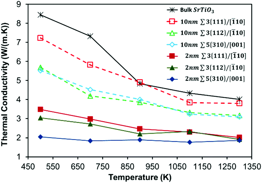 | ||
| Fig. 2 Total thermal conductivities of interacting (2 nm-GB) and non-interacting (10 nm-GB) grain boundaries compared with that of bulk SrTiO3. | ||
All layered nanostructures containing grain boundaries with less favourable formation energies (Table 3) display lower thermal conductivity at 500 K (Fig. 2) when the inter-boundary distance is either 10 nm or 2 nm. No significant correlation is seen otherwise. One can picture this in terms of structural complexity (section 3.1). Grain boundaries with a higher number of distinct coordination environments show the greatest difference in bonding with respect to bulk SrTiO3, and will be less stable and hence have a higher formation energy. It is clear that a greater variety of environments generates a larger number of optical vibrational modes that can couple with the heat transporting acoustic phonons, reducing thermal conductivity. However, the structural complexity is an intricate interplay between four different factors (i.e. distance between the grain boundaries, density of the grain boundary, number of SrTiO3 unit missing at the grain boundary, and dangling bonds per unit area), where these factors are interdependent and not mutually exclusive.
It is clear from Fig. 2 that the introduction of grain boundaries reduces the thermal conductivity compared to stoichiometric bulk SrTiO3, and this is more pronounced when the inter-boundary distance is shorter (i.e. 2 nm-GB have a lower thermal conductivity than 10 nm-GB configurations). The reduction in thermal conductivity when the inter-boundary distance is 10 nm compared to 2 nm is approximately 55%, 45%, and 65% at 500 K for Σ3{111}/[10], Σ3{112}/[10] and Σ5{310}/[001], respectively. As discussed in the next section, the peaks of the HFACF spectra, each corresponds to a vibrational mode. The spectra for 2 nm-GB have more peaks compared to the spectra for 10 nm-GB (Fig. S5†), displaying more vibrational modes, and thus a reduction of thermal conductivity (Fig. 2).
The dangling bond density seems to mostly affect systems with large inter-boundary distance. One would indeed expect for the same inter-boundary distance that is large enough to minimize the boundary–boundary interactions, that the structure of the grain boundary itself (in terms of the dangling bond density) would influence the thermal conductivity. We see this as the thermal conductivity for systems with a large inter-boundary distance, i.e. 10 nm-GB, follows the order Σ3{111}/[10] > Σ3{112}/[10] ≈ Σ5{310}/[001] (Fig. 2). Indeed Σ3{111}/[10] has no dangling bonds and Σ3{112}/[10] and Σ5{310}/[001] have relatively similar densities, 27.0 and 29.4 dangling bonds per nm2. This is also confirmed by the in-plane (i.e. parallel to the grain boundary) contribution to the thermal conductivity (Fig. S4c and S4e†) for Σ3{112}/[10] and Σ5{310}/[001] grain boundaries, which show a relatively similar behaviour. For systems where the grain boundaries are 10 nm apart, we also see that the density of Σ3{112}/[10] and Σ5{310}/[001] are closer to each other and smaller than the density of Σ3{111}/[10]. This trend is similar to the trend seen for their thermal conductivity (Fig. 2).
When the inter-boundary distance decreases and the two grain boundaries become closer (i.e. 2 nm-GB), it appears that the structure of the grain boundary in terms of the dangling bond density is no longer sufficient to explain the change in the thermal conductivity. So one has to discuss the change in thermal conductivity in terms of other structural descriptors (i.e. density of the grain boundary systems, and number of SrTiO3 unit missing at the grain boundary).
For the inter-boundary distance of 10 nm, the density of Σ3{111}/[10] is higher than that of Σ3{112}/[10] and Σ5{310}/[001], and so its thermal conductivity. For 2 nm-GB, the order of thermal conductivity is Σ3{111}/[10] followed by Σ3{112}/[10] and Σ5{310}/[001]. For these 2 nm-GB systems, the density of Σ3{111}/[10] and Σ3{112}/[10]) are relatively similar (Table 1) but much higher than the density of Σ5{310}/[001]. This trend in density seems to follow the trend seen in the thermal conductivity for these structures (Fig. 2). For 2 nm-GB systems the missing SrTiO3 units per nm2, related to the density descriptor, also becomes important. It follows the order Σ3{111}/[10] < Σ3{112}/[10] < Σ5{310}/[001] (Table 2), which has the opposite trend compared to the thermal conductivity of the systems with inter-boundary distance of 2 nm. The 2 nm-GB Σ5{310}/[001] has the lowest density and thus the lowest thermal conductivity. At parity of grain boundary structural complexity (in terms of dangling bond density), the 2 nm-GB Σ3{112}/[10] has a higher density than 2 nm-GB Σ5{310}/[001], and thus a higher thermal conductivity. This is also supported by the in-plane and out-of-plane contributions to the thermal conductivity (Fig. S4d and S4f†), which are very different for the two grain boundaries. This is not the case for the 10 nm-GB Σ5{310}/[001] and Σ3{112}/[10], where the out-of-plane and the in-plane contributions to the total thermal conductivity are similar (Fig. S4c and S4e†).
The effect of structural complexity on the average thermal conductivity fades away as the temperature increases (Fig. 2). This is a general feature in common to all layered nanostructures as it does in the bulk material (Fig. 2). The behaviour seems to be more marked in 10 nm-GB compared to 2 nm-GB systems. At 1300 K, 2 nm-GB systems have all converged to a total thermal conductivity of ∼2 W (m K)−1 and 10 nm-GB systems to a value of ∼3.7 W (m K)−1. This stems from the increase in Umklapp (phonon–phonon) scattering processes at higher temperatures. The acoustic phonons are scattered by other acoustic phonons before they encounter the grain boundaries and so the significance of the particular structure of the boundary diminishes. We attribute the difference between 2 nm-GB and 10 nm-GB systems to the longer allowed wavelength between the boundaries. This effect is well known and is explained by Dove78 and Schelling et al.79 As the temperature dependence in thermal conductivity is less pronounced in 2 nm-GB systems, this suggests indeed a predominant boundary–boundary interaction due to a higher density of scattering centres (i.e. grain boundaries) per unit volume.
On a final note, we do not see any correlation between the value of sigma (Σ) and thermal conductivity but we also only consider three grain boundaries. However, it may be that sigma might not be a universal descriptor as demonstrated by the two Σ3 grain boundaries, which show different behaviour. As mentioned in section 3.1 and 3.2, this suggests that the local coordination environments at the grain boundaries may have a greater impact on thermal conductivity and thus any correlation between thermal conductivity and structure may be more appropriate to draw rather than the use of Σ.
Our computed average thermal conductivities lead to the intriguing prediction that layered nanostructures (with an inter-boundary distance less than 10 nm) of SrTiO3 will be needed to show a desired reduction of thermal conductivity to well below the bulk value. It is therefore clear that in the case of SrTiO3, micron-sized layers are not sufficient to reduce their thermal transport to a level that would show a marked improvement of their thermoelectric performance. Furthermore, a simple comparison between thermal conductivities of different layered nanostructures (Fig. 2) appears to be a straightforward route to identify those nanostructures (i.e. grain boundaries) that experimental work should seek to synthesise. In terms of thermal conductivity, for a thermoelectric material, an optimal structure will be one that shows the largest reduction in thermal conductivity compared to the bulk material, and is also constant as a function of temperature. Our analysis indicates that the layered nanostructure 2 nm-GB Σ5{310}/[001] may be the optimum.
3.3 The in-plane and out-of-plane thermal conductivities of SrTiO3 layered nanostructures
Implementation of thermoelectric materials with nanoscale structural features in thermoelectric devices must consider the directional dependency of the property. For our layered nanostructures, we have therefore separated the in-plane (‖), i.e. parallel to the grain boundary plane (YZ – Fig. 1), and out-of-plane (⊥), i.e. perpendicular to the grain boundary plane (X – Fig. 1), contributions to the thermal conductivity.We found that for the majority of grain boundaries, the out-of-plane (⊥) thermal conductivity is lower than the in-plane (‖) (Fig. S4†), as phonons across the boundary are reduced the most due to a large variety of coordination environments (i.e. scattering centres).60 The only exception is for 10 nm-GB Σ3{111}/[10]. This is most likely related to the coordination of species at the grain boundary, which is similar to the one in bulk SrTiO3 (i.e. Ti is 6 fold coordinated and Sr is 12 fold coordinated). This appears to result in long-lived optical vibrational modes as demonstrated by the narrow peaks in the HFACF spectrum (Fig. S5†). As the in-plane HFACF spectrum has peaks that are sharper than those shown by the out-of-plane HFACF spectrum, this results in a lower in-plane contribution to the thermal conductivity compared to the out-of-plane. These long-lived optical modes indeed do not scatter acoustic vibrational modes as frequently as shorter lifetime optical vibrational modes, resulting in higher thermal conductivity through (i.e. out-of-plane) the grain boundary.78
Therefore, we can conclude that in general for layered nanostructures of SrTiO3, a smaller inter-boundary distance will be desirable to maximise the reduction in thermal conductivity.
3.4 Vibrational response of simulated structures
It is clear that if we are to gain a better control on the thermal conductivity, i.e. control the measurable macroscopic property, there is a need to manipulate the structure of the interfaces. Thus, we need atom level structural details that can be linked to the macroscopic property.We therefore propose a computational protocol that can identify the vibrational responses of nanoscale structural features in these layered nanostructures, but it has no conceptual limitation in its application to any nanostructure. This protocol provides a useful tool to analyse data from molecular dynamics calculations as shown for 3D assemblages of nanocubes of SrTiO3.14 If we consider the spectrum of the heat-flux autocorrelation function (HFACF), it displays characteristic peaks corresponding to Γ-point vibrational modes, the presence of which contributes to increased phonon–phonon scattering.61,62 This can be compared to the phonon density of states (PDOS) calculated using lattice dynamics calculations. An example for bulk SrTiO3 is provided in Fig. 3. The importance of this comparison is that LD calculations provide the eigenvectors corresponding to the atom-level motions associated with each vibrational mode (details in section S1†), and thus a direct route to identify the species and their location involved in each vibrational mode. This analysis provides quantitative information to define the regions within the layered nanostructure, which require further engineering to lower the thermal conductivity.
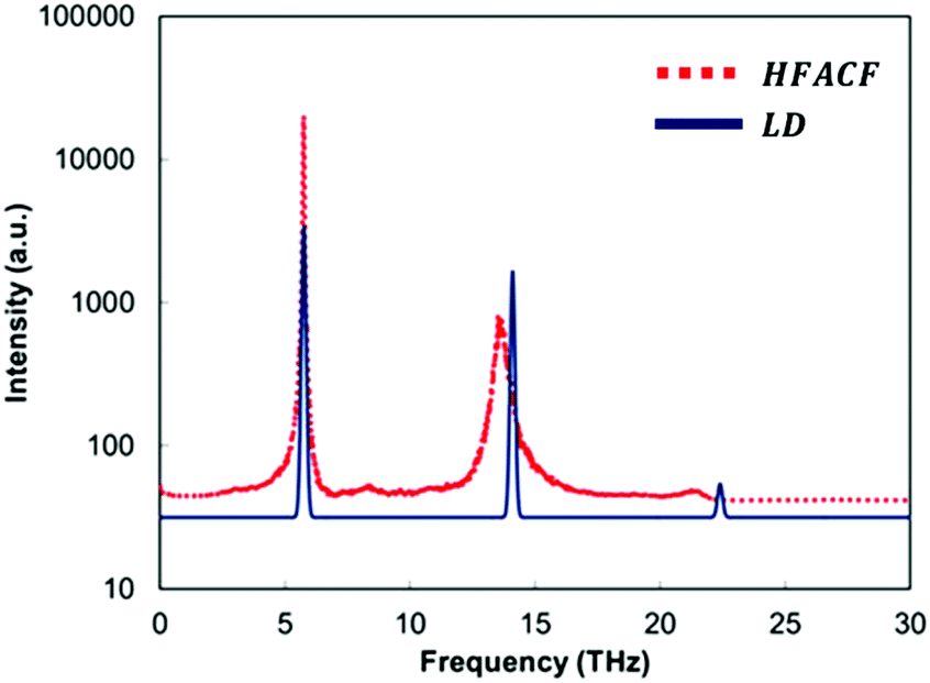 | ||
| Fig. 3 Lattice dynamics (LD) phonon density of state (PDOS) calculated neglecting the effect of temperature, and the heat-flux autocorrelation functions (HFACF) spectrum at 500 K of bulk SrTiO3. Intensities are assigned based on the magnitude of the eigenvector sum for each vibrational mode for LD. Intensities in arbitrary units and log10 scale for HFACF. | ||
Particular attention must be paid to the optical phonon modes appearing at lower frequencies. Due to the Bose–Einstein distribution of phonons across frequencies, there is a larger occupation of acoustic vibrational modes at lower frequencies than higher frequencies.78,80 To effectively scatter these low frequency acoustic modes and lower the thermal conductivity, it is ideal to generate new optical vibrational modes at these low frequencies.
There is a further advantage in determining HFACF spectra of nanostructured materials via molecular dynamics simulations, as they can directly provide some features of the IR spectra, and unlike the PDOS, readily give the peak width of each mode. Although, molecular dynamics simulations can only be at the Γ-point as all periodic images are vibrating in phase with each other, the peaks of a HFACF spectrum correspond to a specific subset of Γ-point optical vibrational modes that will be IR active modes in polar materials.14,60,61 The criterion established by Landry et al.61 requires that the sum of each atom's eigenvectors (i.e. representing the displacement of the vibration) multiplied by the corresponding atom's average energy, must be non-zero for a given vibrational mode to appear in the HFACF spectrum. Landry's criterion is identical to the IR selection rule requiring a change in dipole for a mode to be IR active if the multiplication by the atom's average energy is replaced by the atom's charge. It can therefore be inferred that the modes appearing in the HFACF spectrum will also be IR active modes in polar materials. Indeed, the peaks appearing in the HFACF spectra of stoichiometric bulk SrTiO3 are IR active modes.14
The appearance of peaks, corresponding to optical modes, in the HFACF spectra (Fig. 4) allows direct evidence of the significant contribution of optical vibrational modes to the heat-flux, whereas acoustic vibrational modes are responsible for the long range transport of energy.81 Thus, the scattering of acoustic phonons by optical phonons cannot be ignored and constitutes an important contribution towards the lowering of the thermal conductivity.
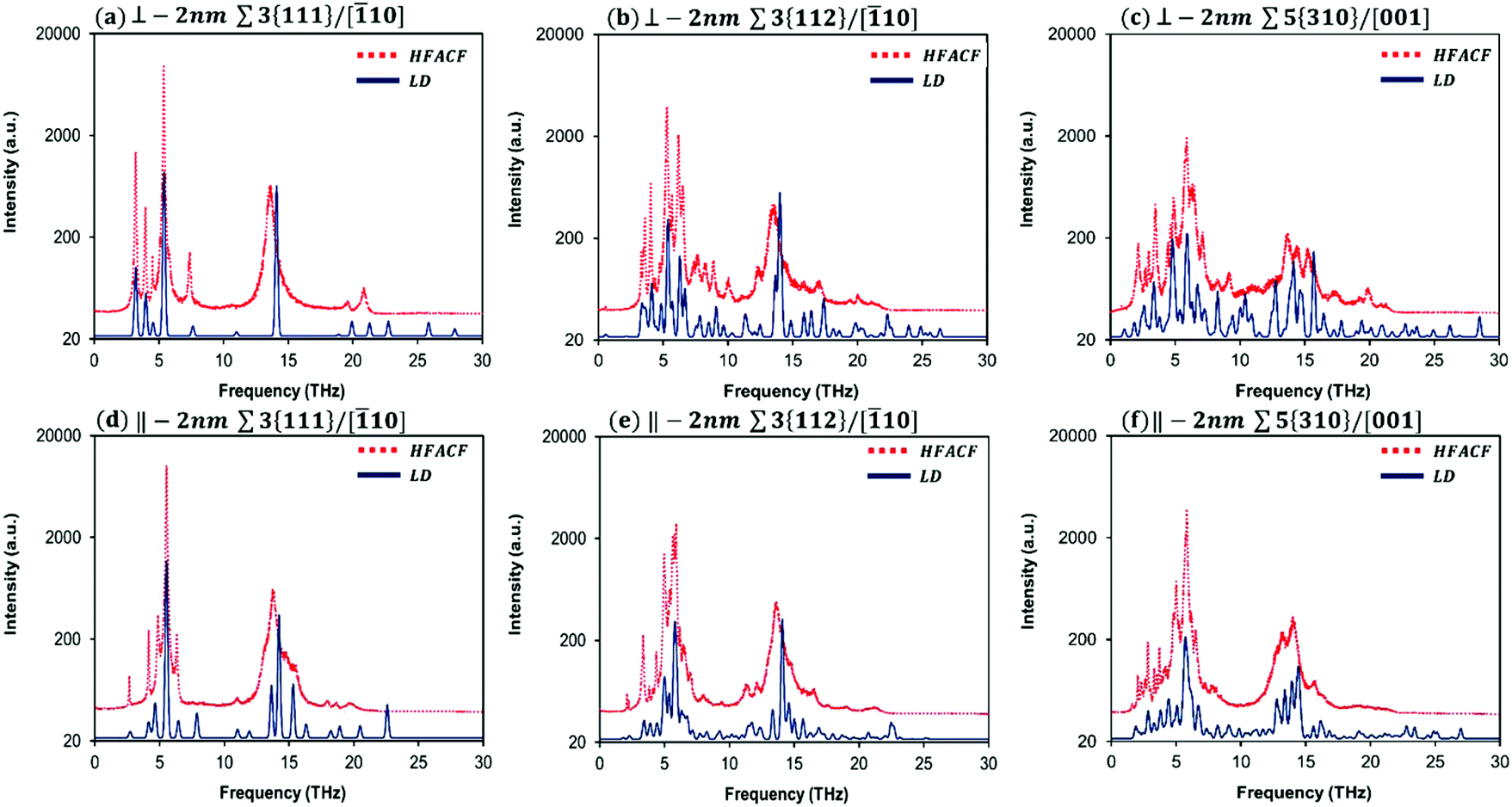 | ||
| Fig. 4 Lattice dynamics (LD) phonon density of state (PDOS) calculated neglecting the effect of temperature, and the heat-flux autocorrelation functions (HFACF) spectrum at 500 K for the 2 nm-GB Σ3{111}/[10], Σ3{112}/[10] and Σ5{310}/[001] grain boundaries. The in-plane (‖) and out-of-plane (⊥) directional vibrational components are separated for each grain boundary. Intensities are assigned based on the magnitude of the eigenvector sum for each vibrational mode for LD. Intensities in arbitrary units and log10 scale for HFACF. | ||
Before discussing the vibrational response of grain boundaries, we explain the procedure on stoichiometric bulk SrTiO3.
For our purpose, we present only the HFACF spectra at 500 K for 2 nm-GB (Fig. 4) and in this case, we distinguish explicitly between the in-plane (‖) and out-of-plane (⊥) vibrational contributions. These spectra show a number of new features (i.e. peaks) compared to the spectrum of bulk SrTiO3 (Fig. 3). It is worth emphasising that a HFACF spectrum with more and/or broader peaks generates a lower thermal conductivity. This is further demonstrated by the HFACF spectra at 500 K for 10 nm-GB that contain generally a lower number of peaks compared to 2 nm-GB systems (Fig. S5†).
To identify the underlying vibrational motions and corresponding species of the new peaks in the HFACF spectra of 2 nm-GB layered nanostructures, we compared the HFACF spectra with the PDOS of LD-GB for each configuration individually (Fig. 4) as we have done for bulk SrTiO3 (Fig. 3). Both 2 nm-GB and LD-GB layered nanostructures have the same inter-boundary distance, which provides a more appropriate comparison between data arising from two different techniques (i.e. molecular dynamics and lattice dynamics).
There is a good agreement between PDOS and HFACF spectra, both in the position and relative intensity of the peaks (Fig. 4). The regions of Sr, Ti and O vibrations display many peaks in the PDOS, which are generally grouped in broad peaks in the HFACF spectra, indicating that many of the underlying motions are concerted. The number of peaks increases with increasing the complexity of the structure, in order Σ3{111}/[10], Σ3{112}/[10] and Σ5{310}/[001]. Hereafter, we present a summary of our findings, whereas a detailed analysis of each vibrational mode (i.e. peak) is presented in Tables S2–S4.†
From a computational viewpoint, as we work towards an approach for predicting compositions and structures that lower thermal conductivity, we need to provide a quantitative analysis of the vibrational modes. We have therefore analysed all the vibrational motions shown in Fig. 4 (listed in Tables S2–S4†) and presented the results in Fig. 5. Although the majority of the vibrational modes within the SrTiO3 layered nanostructures exhibit complex motions, there are some general features, which we can draw out. We have firstly divided the frequencies into three ranges (i.e. 0–10, 10–20 and 20–30 THz), and then identified the percentage vibrational modes in each frequency range that showed a different characteristic, whether in terms of (a) the direction of the mode relative to the grain boundary orientation, (b) the region or location where the mode is most active, and (3) the species which is most active in each mode. This information can be gained by analysing the eigenvectors associated with each atom in the simulation cell for each vibrational mode.
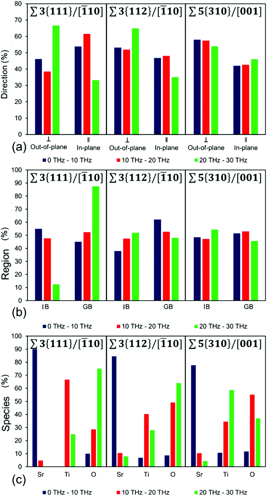 | ||
| Fig. 5 Percentage of vibrational modes analysed depending on (a) direction (in-plane and out-of-plane), (b) region (inter-boundary IB, and grain boundary GB) and (c) species (Sr, Ti and O species), that have a dominant contribution to the vibration, for Σ3{111}/[10], Σ3{112}/[10] and Σ5{310}/[001] grain boundaries in three frequency range. Note: The dominant direction has been normalized to account for the in-plane (‖) contribution consisting of two directions parallel to the grain boundary (i.e. y and z), whereas the out-of-plane (⊥) only of one direction across the grain boundary (i.e. x). | ||
Mathematical details of calculations of these three quantities are in ESI section S2.† The analysis is presented in Fig. 5, where Fig. 5(a) shows percentage of modes in the three frequency ranges that are scattered largely in-plane (parallel) or out-of-plane (perpendicular) to the grain boundary plane, Fig. 5(b) shows the percentage of modes scattered predominantly in the grain boundary (GB) or in the inter-boundary (IB) regions, and Fig. 5(c) shows the scattering in the three frequency ranges according to species, so whether Sr, Ti or O species were involved in the scattering of phonons.
The analysis in Fig. 5(a) shows the percentage of vibrational modes that have a predominant in-plane and an out-of-plane character for each of the layered nanostructures in the three frequency ranges studied (i.e. 0–10, 10–20 and 20–30 THz). The percentage of out-of-plane modes, calculated by summing those vibrational modes with a total eigenvector perpendicular to the grain boundary is generally higher than the percentage of in-plane modes (sum of vibrational modes with a total eigenvector parallel to the grain boundary). It is worth noting that this correlation also matches the relationship between in-plane and out-of-plane contribution to the thermal conductivity (Fig. S5(b), S5(d), S5(f)†) for the three grain boundaries, where the out-of-plane contribution is lower than the in-plane contribution to the thermal conductivity. However, whereas this holds for Σ3{112}/[10] and Σ5{310}/[001], Σ3{111}/[10] does not seem to conform. Unlike the other two grain boundaries studied, this boundary shows a higher percentage of vibrational modes with dominant in-plane character compared to those that have a dominant out-of-plane character, at least for frequencies lower than 20 THz. Thus, one would expect that the in-plane contribution to the thermal conductivity would be higher than the out-of-plane contribution. This is not the case as shown in Fig. S5(b),† where the opposite is seen. It is clear that this discrepancy is due to its structural complexity (section 3.1) as at the boundary, the nanostructure does not show any dangling bonds (i.e. all the species at the grain boundary are fully coordinated), there is a relatively high density compared to the other two grain boundaries (as demonstrated by the number of SrTiO3 units per nm2, 0.48 per nm2). Examination of Fig. 4(a) and (d), which show the in-plane (‖) and out-of-plane (⊥) HFACF spectra at 500 K for 2 nm-GB Σ3{111}/[10], can shed some light onto our finding. Although the vibrational modes in Fig. 4(a) and (d) are within the same range of frequencies, the modes in Fig. 4(a) are generally concentrated below the main Sr peak (i.e. 5 THz), whereas in Fig. 4(d) they are more evenly distributed across the whole range of frequencies. Therefore, even though below 20 THz there are more peaks with in-plane character, the peaks with out-of-plane character are more effective at scattering acoustic phonons due to their low frequency (i.e. below 5 THz) and the larger occupation of low frequency acoustic phonons due to the Bose–Einstein distribution.78,80
Fig. 5(b) shows the percentage of vibrational modes that have a predominant grain boundary or inter-boundary character for each of the layered nanostructures in the three frequency ranges studied. This means that all the vibrational modes with a total eigenvector that arises with a greater contribution from species located at the grain boundary are considered to have a predominant grain boundary (GB) character, whereas all the vibrational modes with a total eigenvector that arises with a greater contribution from species located in the inter-boundary region are considered to have a predominant inter-boundary (IB) character. The region contribution (Fig. 5(b)) shows that the vibrational modes may have a predominant grain boundary (GB) or inter-boundary (IB) character. This arises from the fact that the IB and GB regions are structurally different. In the GB region some of the species have local coordination environments that are different from Sr, Ti and O species in bulk SrTiO3, whereas all the species in the IB region have local coordination environments for Sr, Ti and O species that are the same as in bulk SrTiO3. Our analysis shows that the largest contribution to the total percentage of vibrational modes arises generally from both the IB and the GB regions (Fig. 5(b)). This further supports that as noted previously all the vibrational modes for these layered nanostructures are complex motions where species in the IB and GB regions both contribute to the scattering of phonons at all frequencies. There are however some peculiar difference between the different nanostructures. Σ3{111}/[10] grain boundary shows that the dominant contribution in the region below 10 THz arises from the inter-boundary region, whereas Σ5{310}/[001] has almost identical contributions from the inter-boundary and the grain boundary regions throughout the entire range of frequencies (0–30 THz).
Fig. 5(c) shows the percentage of vibrational modes that have a predominant Sr or Ti or O (i.e. different species) character in the three frequency ranges studied. This means that all the vibrational modes with a total eigenvector that arises from a greater contribution from Sr species are labelled as “Sr”, those with a greater contribution form Ti species are labelled as “Ti”, and those with a greater contribution from O species are labelled as “O”. Analysis of the contribution of vibrational modes from the different species (Fig. 5(c)) indicates that for all the frequency ranges studied (i.e. 0–10, 10–20 and 20–30 THz) the vibrational mode is always characterized by the vibration of a dominant species (i.e. Sr, Ti or O). For bulk SrTiO3 (Fig. 3 and section 3.4.1), the region below 10 THz was defined by Sr vibrations, between 10–20 THz by Ti vibrations and above 20 THz by O vibrations. However this division does not hold for all the layered nanostructures, reiterating that the vibrations are indeed complex modes due to the presence of the grain boundary. It still holds for Σ3{111}/[10], but for Σ3{112}/[10] and Σ5{310}/[001], only the region below 10 THz is dominated by Sr vibrations. As the complexity of the structure and coordination of species at the grain boundary increases, the frequencies above 10 THz become a mixture of Ti and O vibrations. In these two boundaries there is also a larger number of Ti vibrations below 10 THz compared to the Σ3{111}/[10] boundary.
3.5 Implication for nanostructuring SrTiO3
Our data collected for layered nanostructures shows that those with grain boundaries that display a greater number of features in the HFACF spectra, have lower thermal conductivity, i.e. in order Σ3{111}/[10], Σ3{112}/[10] and Σ5{310}/[001]. Inspection of the vibrational modes from lattice dynamics calculations allows for the identification of the nature of the species, whether Sr, Ti or O (Fig. 5(c)), that is vibrating, and their physical location within the layered nanostructure, whether the species reside at the grain boundary or in the inter-boundary region (Fig. 5(b)). Thus, there are two implications when considering any manipulation of these nanostructures to further reduce the thermal conductivity.
One is a compositional factor. In this case, although the variety of Sr and Ti environments in grain boundaries promotes new vibrations, three vibrational regions are still distinguishable at frequencies close to the characteristic Sr (∼5 THz), Ti (∼14 THz) and O (∼20 THz) vibrational frequencies of bulk SrTiO3. This is of particular advantage as it reduces the complexity of any consideration to further reduce the thermal conductivity.
The other is a structural factor (i.e. the structure of the grain boundary). Our analysis shows that as the complexity of any nanoscale structural feature increases, the number of complex vibrations also increases (Fig. 4 and 2). These vibrations involve species that are located in both inter-boundary and grain boundary regions, but in the majority of cases, the contribution of one region dominates (Fig. 5(b)). Generally, within the three identified regions of Sr, Ti and O vibrations, those with a more inter-boundary character are the more intense (i.e. highest and broader peaks in Fig. 4).
Our computational analysis shows that nanostructuring SrTiO3 can indeed lower thermal conductivity, and that this arises from considerations on the species that are vibrating and their location within the nanostructure. It is clear that to gain the best result, knowledge of the structures of grain boundaries that are introduced in the layered nanostructure is invaluable. Our results show that our computational framework can provide atom level details and their corresponding vibrational response, and that this can be achieved in a routine way using a combination of molecular and lattice dynamics. Therefore, any experimental attempt to lower thermal conductivity of layered nanostructures can in principle be based first on computational guidelines.
Our results show that the choice of grain boundary structure influences the thermal conductivity, with a more dense and stable Σ3{111}/[10] structure showing higher thermal conductivity than a less dense and less stable Σ5{310}/[001] structure. From an experimental viewpoint, it will be worth focusing on techniques that can control the structure of the interfaces within the nanostructured material.71,75,87,88 Furthermore, annealing of samples should be performed at lower temperature and for a reduced time to limit grain growth and ensure that higher index (i.e. less stable) surfaces and interfaces will be present.
Our results also show that as the inter-boundary distance between the grain boundaries decreases so does the thermal conductivity, and also that for inter-boundary distances of 2 nm the out-of-plane contribution of the thermal conductivity is lower than the in-plane contribution (Fig. S4†). Thus any enhanced phonon scattering should target the inter-boundary region rather than the grain boundary region. This can be achieved by choosing dopant that do not segregate to grain boundaries.
4. Conclusions
We developed a computational protocol, combining lattice and molecular dynamics calculations, to examine the relationship between the structure of layered nanostructures containing specific tilt grain boundaries of an important thermoelectric material, SrTiO3, and their thermal conductivities.Analysis of the phonon density of state (PDOS) and the heat-flux autocorrelation function (HFACF) spectrum for each solid interface provides evidence that there are two factors controlling the thermal conductivity at the boundary: one is the composition and the other is the coordination of boundary species.
The vibrational response of the tilt grain boundaries in SrTiO3 layered nanostructures is characterized by complex vibrational modes that involve both species at the grain boundary and in the inter-boundary region. Increased structural complexity results in an increased number of these modes and provides a more efficient scattering of phonons. This allow for the reduction of thermal conductivity, which for our tilt boundaries follows the order Σ3{111}/[10], Σ3{112}/[10] and Σ5{310}/[001]. Furthermore, when phonon-boundary scattering becomes the dominant process over the phonon–phonon scattering, the thermal conductivity lowers further and for Σ5{310}/[001] it results in a near constant thermal conductivity as a function of temperature.
Finally, future work should include a larger scale investigation over a broader selection of grain boundaries as a function of their Σ value, should account for the effect of point defects in the space charge layer induced by the presence of grain boundaries, and should be extended to thermoelectric properties such as Seebeck coefficient and electronic conductivity, which along with the thermal conductivity contribute to the thermoelectric efficiency of the material.
Conflicts of interest
There are no conflicts of interest to declare.Acknowledgements
This work has made use of ARCHER, the UK's national HPC, via the Materials Chemistry Consortium funded by the EPSRC (EP/L000202), in addition to the HPC Balena at the University of Bath, the HPC Orion at the University of Huddersfield, and the HPC Hydra and HPC Athena at Loughborough University. The authors acknowledge the EPSRC (EP/I03601X/1 and EP/K016288/1) for funding. All data supporting this study are openly available from the University of Bath data archive.References
- K. Biswas, J. He, I. D. Blum, C.-I. Wu, T. P. Hogan, D. N. Seidman, V. P. Dravid and M. G. Kanatzidis, Nature, 2012, 489, 414–418 CrossRef PubMed.
- D. G. Cahill, W. K. Ford, K. E. Goodson, G. D. Mahan, A. Majumdar, H. J. Maris, R. Merlin and S. R. Phillpot, J. Appl. Phys., 2003, 93, 793–818 CrossRef.
- K. Koumoto, Y. F. Wang, R. Z. Zhang, A. Kosuga and R. Funahashi, Annu. Rev. Mater. Res., 2010, 40, 363–394 CrossRef.
- R. Liu, J. Duay and S. B. Lee, Chem. Commun., 2011, 47, 1384–1404 RSC.
- B. Poudel, Q. Hao, Y. Ma, Y. Lan, A. Minnich, B. Yu, X. Yan, D. Wang, A. Muto, D. Vashaee, X. Chen, J. Liu, M. S. Dresselhaus, G. Chen and Z. Ren, Science, 2008, 320, 634–638 CrossRef PubMed.
- E. S. Toberer, A. Zevalkink and G. J. Snyder, J. Mater. Chem., 2011, 21, 15843–15852 RSC.
- M. Zebarjadi, K. Esfarjani, Z. Bian and A. Shakouri, Nano Lett., 2011, 11, 225–230 CrossRef PubMed.
- G. J. Snyder and E. S. Toberer, Nat. Mater., 2008, 7, 105–114 CrossRef PubMed.
- C. Fu, S. Bai, Y. Liu, Y. Tang, L. Chen, X. Zhao and T. Zhu, Nat. Commun., 2015, 6, 8144 CrossRef PubMed.
- J. D. Baran, M. Molinari, N. Kulwongwit, F. Azough, R. Freer, D. Kepaptsoglou, Q. M. Ramasse and S. C. Parker, J. Phys. Chem. C, 2015, 119, 21818–21827 CrossRef.
- J. D. Baran, D. Kepaptsoglou, M. Molinari, N. Kulwongwit, F. Azough, R. Freer, Q. M. Ramasse and S. C. Parker, Chem. Mater., 2016, 28, 7470–7478 CrossRef.
- M. Molinari, D. A. Tompsett, S. C. Parker, F. Azough and R. Freer, J. Mater. Chem. A, 2014, 2, 14109–14117 RSC.
- D. Selli, S. E. Boulfelfel, P. Schapotschnikow, D. Donadio and S. Leoni, Nanoscale, 2016, 8, 3729–3738 RSC.
- S. R. Yeandel, M. Molinari and S. C. Parker, RSC Adv., 2016, 6, 114069–114077 RSC.
- F. Dang, C. Wan, N.-H. Park, K. Tsuruta, W.-S. Seo and K. Koumoto, ACS Appl. Mater. Interfaces, 2013, 5, 10933–10937 CrossRef PubMed.
- R.-Z. Zhang, C.-L. Wang, J.-C. Li and K. Koumoto, J. Am. Ceram. Soc., 2010, 93, 1677–1681 Search PubMed.
- Y. Lin, C. Norman, D. Srivastava, F. Azough, L. Wang, M. Robbins, K. Simpson, R. Freer and I. A. Kinloch, ACS Appl. Mater. Interfaces, 2015, 7, 15898–15908 CrossRef PubMed.
- J. Wang, S. Choudhary, W. L. Harrigan, A. J. Crosby, K. R. Kittilstved and S. S. Nonnenmann, ACS Appl. Mater. Interfaces, 2017, 9, 10847–10854 CrossRef PubMed.
- S.-Y. Choi, S.-D. Kim, M. Choi, H.-S. Lee, J. Ryu, N. Shibata, T. Mizoguchi, E. Tochigi, T. Yamamoto, S.-J. L. Kang and Y. Ikuhara, Nano Lett., 2015, 15, 4129–4134 CrossRef PubMed.
- X. Wu and T. Luo, J. Appl. Phys., 2014, 115, 014901 CrossRef.
- M. D. Losego, M. E. Grady, N. R. Sottos, D. G. Cahill and P. V. Braun, Nat. Mater., 2012, 11, 502–506 CrossRef PubMed.
- P. Yang, H. Xu, L. Zhang, F. Xie and J. Yang, ACS Appl. Mater. Interfaces, 2012, 4, 158–162 CrossRef PubMed.
- S. P. Waldow and R. A. De Souza, ACS Appl. Mater. Interfaces, 2016, 8, 12246–12256 CrossRef PubMed.
- Z. Wang, J. E. Alaniz, W. Jang, J. E. Garay and C. Dames, Nano Lett., 2011, 11, 2206–2213 CrossRef PubMed.
- A. Bagri, S.-P. Kim, R. S. Ruoff and V. B. Shenoy, Nano Lett., 2011, 11, 3917–3921 CrossRef PubMed.
- Z. Zheng, X. Chen, B. Deng, A. Chernatynskiy, S. Yang, L. Xiong and Y. Chen, J. Appl. Phys., 2014, 116, 073706 CrossRef.
- W.-L. Tzeng, T.-L. Sun and S.-J. Shih, Adv. Powder Technol., 2016, 27, 799–807 CrossRef.
- C. Hou, W. Huang, W. Zhao, D. Zhang, Y. Yin and X. Li, ACS Appl. Mater. Interfaces, 2017, 9, 20484–20490 CrossRef PubMed.
- E.-J. Guo, T. Charlton, H. Ambaye, R. D. Desautels, H. N. Lee and M. R. Fitzsimmons, ACS Appl. Mater. Interfaces, 2017, 9, 19307–19312 CrossRef PubMed.
- S. A. Lee, J.-Y. Hwang, E. S. Kim, S. W. Kim and W. S. Choi, ACS Appl. Mater. Interfaces, 2017, 9, 3246–3250 CrossRef PubMed.
- D. J. Baek, D. Lu, Y. Hikita, H. Y. Hwang and L. F. Kourkoutis, ACS Appl. Mater. Interfaces, 2017, 9, 54–59 CrossRef PubMed.
- G. G. Yadav, G. Zhang, B. Qiu, J. A. Susoreny, X. Ruan and Y. Wu, Nanoscale, 2011, 3, 4078–4081 RSC.
- M. L. Reinle-Schmitt, C. Cancellieri, A. Cavallaro, G. F. Harrington, S. J. Leake, E. Pomjakushina, J. A. Kilner and P. R. Willmott, Nanoscale, 2014, 6, 2598–2602 RSC.
- E. Ahvenniemi and M. Karppinen, Chem. Mater., 2016, 28, 6260–6265 CrossRef.
- M. Nisula and M. Karppinen, Nano Lett., 2016, 16, 1276–1281 CrossRef PubMed.
- R. H. A. Ras, E. Sahramo, J. Malm, J. Raula and M. Karppinen, J. Am. Chem. Soc., 2008, 130, 11252–11253 CrossRef PubMed.
- V. Varshney, S. S. Patnaik, A. K. Roy, G. Froudakis and B. L. Farmer, ACS Nano, 2010, 4, 1153–1161 CrossRef PubMed.
- Y.-Y. Zhang, Q.-X. Pei, J.-W. Jiang, N. Wei and Y.-W. Zhang, Nanoscale, 2016, 8, 483–491 RSC.
- G. Qin, Z. Qin, W.-Z. Fang, L.-C. Zhang, S.-Y. Yue, Q.-B. Yan, M. Hu and G. Su, Nanoscale, 2016, 8, 11306–11319 RSC.
- V. Varshney, A. K. Roy, G. Froudakis and B. L. Farmer, Nanoscale, 2011, 3, 3679–3684 RSC.
- Z. Luo, J. Maassen, Y. Deng, Y. Du, R. P. Garrelts, M. S. Lundstrom, P. D. Ye and X. Xu, Nat. Commun., 2015, 6, 8572 CrossRef PubMed.
- N. Song, D. Jiao, S. Cui, X. Hou, P. Ding and L. Shi, ACS Appl. Mater. Interfaces, 2017, 9, 2924–2932 CrossRef PubMed.
- J. Fang, C. Reitz, T. Brezesinski, E. J. Nemanick, C. B. Kang, S. H. Tolbert and L. Pilon, J. Phys. Chem. C, 2011, 115, 14606–14614 CrossRef.
- N. R. Williams, M. Molinari, S. C. Parker and M. T. Storr, J. Nucl. Mater., 2015, 458, 45–55 CrossRef.
- G. W. Watson, E. T. Kelsey, N. H. deLeeuw, D. J. Harris and S. C. Parker, J. Chem. Soc., Faraday Trans., 1996, 92, 433–438 RSC.
- S. von Alfthan, N. A. Benedek, L. Chen, A. Chua, D. Cockayne, K. J. Dudeck, C. Elsässer, M. W. Finnis, C. T. Koch and B. Rahmati, Annu. Rev. Mater. Res., 2010, 40, 557–599 CrossRef.
- Y.-M. Chiang and T. Takagi, J. Am. Ceram. Soc., 1990, 73, 3286–3291 CrossRef.
- R. A. De Souza, Phys. Chem. Chem. Phys., 2009, 11, 9939–9969 RSC.
- F. Gunkel, R. Waser, A. H. H. Ramadan, R. A. De Souza, S. Hoffmann-Eifert and R. Dittmann, Phys. Rev. B: Condens. Matter Mater. Phys., 2016, 93, 245431 CrossRef.
- D. Srivastava, F. Azough, M. Molinari, S. C. Parker and R. Freer, J. Electron. Mater., 2015, 44, 1803–1808 CrossRef.
- D. Kepaptsoglou, J. D. Baran, F. Azough, D. Ekren, D. Srivastava, M. Molinari, S. C. Parker, Q. M. Ramasse and R. Freer, Inorg. Chem., 2018, 57, 45–55 CrossRef PubMed.
- P. Canepa, PhD Thesis, University of Kent, 2012 Search PubMed.
- D. Srivastava, F. Azough, R. Freer, E. Combe, R. Funahashi, D. M. Kepaptsoglou, Q. M. Ramasse, M. Molinari, S. R. Yeandel, J. D. Baran and S. C. Parker, J. Mater. Chem. C, 2015, 3, 12245–12259 RSC.
- F. Azough, R. Freer, S. R. Yeandel, J. D. Baran, M. Molinari, S. C. Parker, E. Guilmeau, D. Kepaptsoglou, Q. Ramasse, A. Knox, D. Gregory, D. Paul, M. Paul, A. Montecucco, J. Siviter, P. Mullen, W. Li, G. Han, E. A. Man, H. Baig, T. Mallick, N. Sellami, G. Min and T. Sweet, J. Electron. Mater., 2016, 45, 1894–1899 CrossRef.
- F. Azough, R. J. Cernik, B. Schaffer, D. Kepaptsoglou, Q. M. Ramasse, M. Bigatti, A. Ali, I. MacLaren, J. Barthel, M. Molinari, J. D. Baran, S. C. Parker and R. Freer, Inorg. Chem., 2016, 55, 3338–3350 CrossRef PubMed.
- S. Plimpton, J. Comput. Phys., 1995, 117, 1–19 CrossRef.
- M. S. Green, J. Chem. Phys., 1954, 22, 398–413 CrossRef.
- R. Kubo, J. Phys. Soc. Jpn., 1957, 12, 570–586 CrossRef.
- A. J. H. McGaughey and M. J. Kaviany, presented in part at the 8th AIAA/ASME Joint Thermophysics and Heat Transfer Conference, AIAA-2002-3343, St. Louis, Missouri, 2002.
- A. J. H. McGaughey and M. Kaviany, Int. J. Heat Mass Transfer, 2004, 47, 1799–1816 CrossRef.
- E. S. Landry, M. I. Hussein and A. J. H. McGaughey, Phys. Rev. B: Condens. Matter Mater. Phys., 2008, 77, 184302 CrossRef.
- A. J. H. McGaughey, M. I. Hussein, E. S. Landry, M. Kaviany and G. M. Hulbert, Phys. Rev. B: Condens. Matter Mater. Phys., 2006, 74, 104304 CrossRef.
- C. H. Lee, I. Hase, H. Sugawara, H. Yoshizawa and H. Sato, J. Phys. Soc. Jpn., 2006, 75, 123602 CrossRef.
- A. Togo, F. Oba and I. Tanaka, Phys. Rev. B: Condens. Matter Mater. Phys., 2008, 78, 134106 CrossRef.
- A. Togo, L. Chaput and I. Tanaka, Phys. Rev. B: Condens. Matter Mater. Phys., 2015, 91, 094306 CrossRef.
- J. P. Allen, W. Gren, M. Molinari, C. Arrouvel, F. Maglia and S. C. Parker, Mol. Simul., 2009, 35, 584–608 CrossRef.
- O. Kienzle, M. Exner and F. Ernst, Phys. Status Solidi A, 1998, 166, 57–71 CrossRef.
- S. Hutt, S. Köstlmeier and C. Elsässer, J. Phys.: Condens. Matter, 2001, 13, 3949 CrossRef.
- K. J. Dudeck, N. A. Benedek, M. W. Finnis and D. J. H. Cockayne, Phys. Rev. B: Condens. Matter Mater. Phys., 2010, 81, 134109 CrossRef.
- N. A. Benedek, A. L.-S. Chua, C. Elsässer, A. P. Sutton and M. W. Finnis, Phys. Rev. B: Condens. Matter Mater. Phys., 2008, 78, 064110 CrossRef.
- M. Imaeda, T. Mizoguchi, Y. Sato, H.-S. Lee, S. Findlay, N. Shibata, T. Yamamoto and Y. Ikuhara, Phys. Rev. B: Condens. Matter Mater. Phys., 2008, 78, 245320 CrossRef.
- S. B. Lee, W. Sigle, W. Kurtz and M. Rühle, Acta Mater., 2003, 51, 975–981 CrossRef.
- V. Ravikumar, V. Dravid and D. Wolf, Interface Sci., 2000, 8, 157–175 CrossRef.
- B. Feng, I. Sugiyama, H. Hojo, H. Ohta, N. Shibata and Y. Ikuhara, Sci. Rep., 2016, 6, 20288 CrossRef PubMed.
- N. Shibata, F. Oba, T. Yamamoto and Y. Ikuhara, Philos. Mag., 2004, 84, 2381–2415 CrossRef.
- H. Muta, K. Kurosaki and S. Yamanaka, J. Alloys Compd., 2005, 392, 306–309 CrossRef.
- Y. Wang, K. Fujinami, R. Zhang, C. Wan, N. Wang, Y. Ba and K. Koumoto, Appl. Phys. Express, 2010, 3, 031101 CrossRef.
- M. T. Dove, Structure and Dynamics: An Atomic View of Materials, Oxford University Press, Oxford, 2003 Search PubMed.
- P. K. Schelling, S. R. Phillpot and P. Keblinski, Phys. Rev. B: Condens. Matter Mater. Phys., 2002, 65, 144306 CrossRef.
- M. T. Dove, Introduction to Lattice Dynamics, Cambridge University Press, Cambridge, 1993 Search PubMed.
- Z. Tian, K. Esfarjani, J. Shiomi, A. S. Henry and G. Chen, Appl. Phys. Lett., 2011, 99, 053122 CrossRef.
- W. Zhong, R. D. Kingsmith and D. Vanderbilt, Phys. Rev. Lett., 1994, 72, 3618–3621 CrossRef PubMed.
- S. R. Popuri, A. J. M. Scott, R. A. Downie, M. A. Hall, E. Suard, R. Decourt, M. Pollet and J. W. G. Bos, RSC Adv., 2014, 4, 33720–33723 RSC.
- S. S. Jackson, F. Azough and R. Freer, J. Electron. Mater., 2014, 43, 2331–2336 CrossRef.
- S. R. Phillpot, P. K. Schelling and P. Keblinski, J. Mater. Sci., 2005, 40, 3143–3148 CrossRef.
- P. K. Schelling, S. R. Phillpot and P. Keblinski, J. Appl. Phys., 2004, 95, 6082–6091 CrossRef.
- T. Yamada, N. Wakiya, K. Shinozaki and N. Mizutani, Appl. Phys. Lett., 2003, 83, 4815–4817 CrossRef.
- W. Si, C. Zhang, X. Shi, T. Ozaki, J. Jaroszynski and Q. Li, Appl. Phys. Lett., 2015, 106, 032602 CrossRef.
Footnote |
| † Electronic supplementary information (ESI) available. See DOI: 10.1039/c8nr02234h |
| This journal is © The Royal Society of Chemistry 2018 |