Configuration of the magnetosome chain: a natural magnetic nanoarchitecture

Abstract

Magnetospirillum gryphiswaldense is a microorganism with the ability to biomineralize magnetite nanoparticles, called magnetosomes, and arrange them into a chain that behaves like a magnetic compass. Rather than straight lines, magnetosome chains are slightly bent, as evidenced by electron cryotomography. Our experimental and theoretical results suggest that due to the competition between the magnetocrystalline and shape anisotropies, the effective magnetic moment of individual magnetosomes is tilted out of the [111] crystallographic easy axis of magnetite. This tilt does not affect the direction of the chain net magnetic moment, which remains along the [111] axis, but explains the arrangement of magnetosomes in helical-like shaped chains. Indeed, we demonstrate that the chain shape can be reproduced by considering an interplay between the magnetic dipolar interactions between magnetosomes, ruled by the orientation of the magnetosome magnetic moment, and a lipid/protein-based mechanism, modeled as an elastic recovery force exerted on the magnetosomes.

---

Magnetotactic bacteria (MTB) are microorganisms ubiquitously present in any aquatic environment with the capability of magnetic orientation.¹ The origin of this behavior is due to the presence of intracellular magnetic nanoparticles enclosed in a vesicle, called magnetosomes. The size, morphology and composition of the magnetosomes depend on the species, being the size, in all of them, large enough to be magnetically stable at room temperature.² Most MTB organize the magnetosomes in a chain. Since magnetosomes are single magnetic domains, the chain behaves as a large single permanent dipole magnet which is able to passively reorient the whole bacteria along external magnetic field lines, even at fields as small as those existing near the Earth's surface (≈20–60 μT).^3–5 On top of the fundamental scientific interest of these fascinating microorganisms, magnetosome chains constitute a natural paradigm of highly anisotropic magnetic nanostructures, which show high potentiality in biomedical applications,^6–9 in actuation devices as nanorobots,¹⁰ in nanosensor devices,¹¹ and in magnetic memory devices.¹²

Among all the MTB species, Magnetospirillum gryphiswaldense strain MSR-1 is frequently used as a model strain of MTB due to its ease of cultivation in the laboratory. Magnetospirillum cells are helical and contain a variable number of ∼40–45 nm sized cuboctahedral magnetite (Fe₃O₄) magnetosomes arranged in a chain. The biomineralization of the magnetite nanoparticles and the assembly in a chain are complex and comprise different steps.^4,13,14 Firstly, the magnetosome membrane is formed from the invagination of the cytoplasmic membrane comprised with proteins.¹⁵ Secondly, iron is taken up from the environment and transported into the magnetosome vesicle where nucleation in magnetite nanocrystals occurs,^16–18 and finally, magnetosomes are assembled forming the chain.^4,19–21 The present work is devoted to shed light on this last step. In particular, here we address the underlying mechanisms that determine the arrangement of the magnetosomes and consequently the geometry of the chain.

The arrangement of magnetosomes in a chain results from the interplay between the active assembly mechanism mediated by proteins and the magnetic dipolar interactions between the nearest magnetite nanoparticles.^22–24 As shown by cryotomography imaging on Magnetospirillum, bundles of cytoskeletal filaments intervene in the chain assembly.^15,25,26 These filaments, formed by the actin-like protein MamK, traverse the cell and position the chain in the middle of the cell. Another important protein involved in the chain formation is MamJ. One possible function of MamJ is to connect the magnetosome membrane to the cytoskeletal filament. As magnetosomes get closer together, magnetic dipolar interactions arise.

Here we show by electron cryotomography imaging that magnetosome chains of M. gryphiswaldense are not straight lines but appear slightly bent, a fact that has been also observed in previous studies.^14,26 The implications of the chain shape on the magnetic response of magnetosome chains have then been addressed with complementary techniques performed on a set of bacterial arrangements: (i) small angle neutron/X-ray scattering (SANS/SAXS) on a bacterial colloid, (ii) macroscopic magnetometry on 3D and 2D fixed arrangements of randomly distributed and aligned bacteria, and (iii) X-ray photoemission electron microscopy (XPEEM) on an individual chain of magnetosomes extracted from bacteria.

Two main findings are achieved from this work. Firstly, the equilibrium magnetic moment of the magnetosomes is tilted 20° out of the [111] crystallographic axis, as concluded from the magnetic analysis. Secondly, the tilting of the magnetic moment is the key to understand the helical-like shape of the magnetosome chains. Indeed, the experimental chain patterns imaged by electron cryotomography are accurately reproduced by counterbalancing the magnetic dipolar interactions between magnetosomes, strongly affected by the orientation of the individual magnetic moments, and a lipid/protein-based mechanism, modeled as an elastic recovery force exerted on magnetosomes.

Besides the basic interest of this study, a precise knowledge of the mechanisms determining the chain shape is decisive in applications of MTB such as biological micro-robots. Precisely, recent studies propose MTB to be exploited as motors with embedded source propulsion secured by their flagella and embedded steering system to control the directional motion provided by their magnetosome chain.⁷

Results and discussion

Electron cryotomography imaging of the magnetosome chain

The cells of M. gryphiswaldense have been imaged by electron cryotomography (ECT). Since bacteria are cryoembedded, the cells and as a consequence the magnetosome chains inside them preserve their natural shape, avoiding artifacts associated with cell drying processes. ECT images of two cells are shown in Fig. 1a and b. The upper part of Fig. 1a and b shows the reconstructed 3D tomograms from the tilt-series of images obtained by ECT of the two cells and the insets show the Z-projected images of the tomograms. These projections are equivalent to the images obtained by transmission electron microscopy. The chains shown in Fig. 1 are composed of N = 15 and 22 magnetosomes, respectively, and the mean center-to-center distance between magnetosomes is d ≈ 60 nm. Videos showing the 3D reconstructions of the two magnetosome chains from different perspectives can be found in the ESI (movies S1 and S2†). ECT imaging evidences that magnetosome chains are certainly not straight lines but exhibit more complex patterns. Three slices (XY, YZ and XZ) of each of the 3D reconstructions are shown below the tomograms in Fig. 1a and b. The three slices are cuts of the corresponding tomograms taken along the marked lines and intersect in one of the magnetosomes, so that the XYZ coordinates of that particular magnetosome can be determined. By determining the XYZ coordinates of all the magnetosomes in the chain we have been able to reconstruct the two magnetosome chains, which are shown in Fig. 5b, where a zoom-in of one of the magnetosome chain reconstructions emphasizes the deviation from a straight line.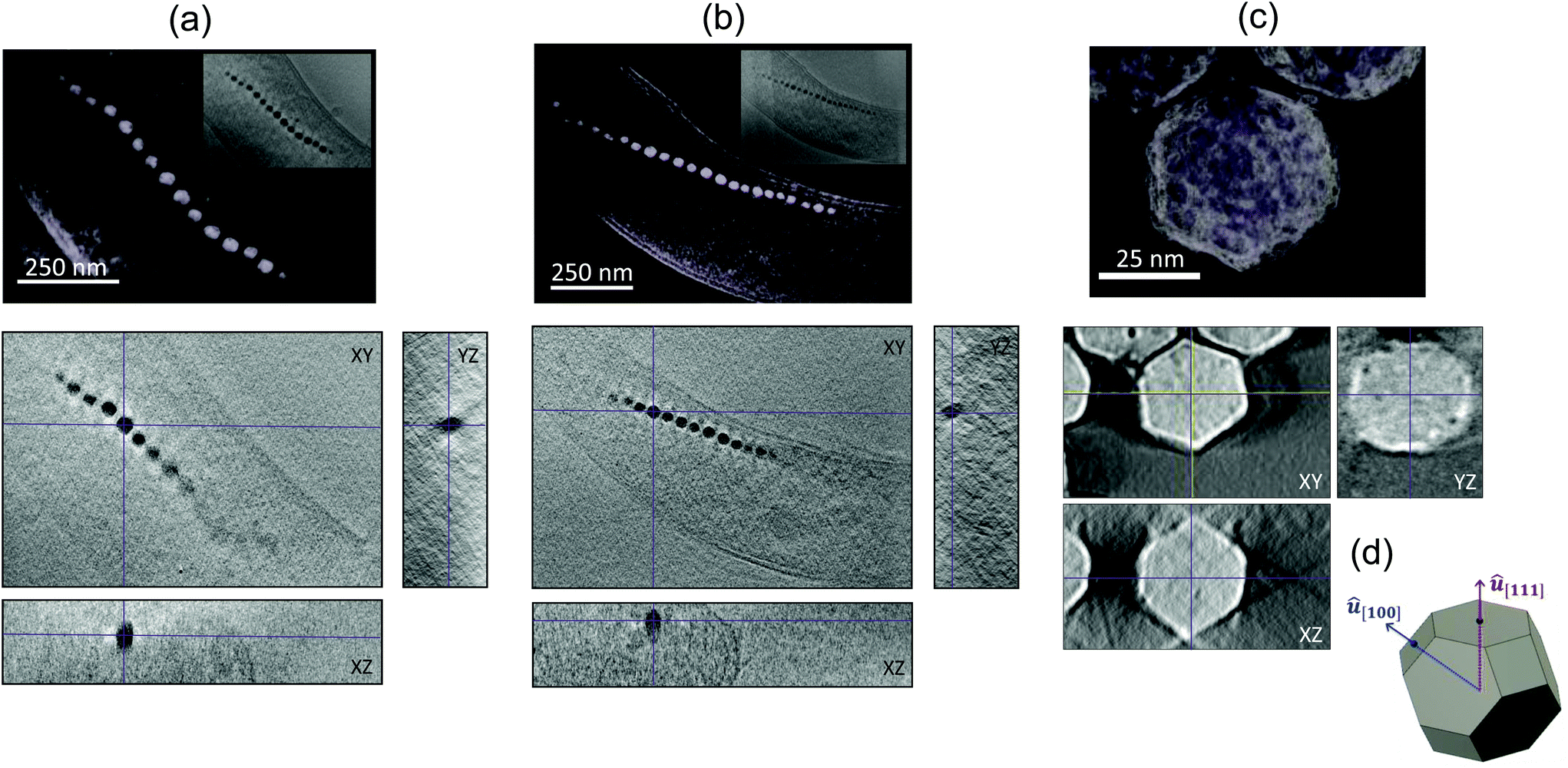

Fig. 1 Electron cryotomography (ECT) of magnetosome chains. (a) and (b) are ECT images of two different bacteria. Top: 3D tomograms reconstructed from the tilt-series of images obtained by ECT. Videos of the tomograms of the two chains viewed from different perspectives (as consecutive slices in XY, XZ and YZ plane orientations, and as an electron density map) can be found in the ESI (movies S1 and S2†). The insets show the Z-projection of the tomograms. Bottom: XY, YZ and XZ slices of the tomograms shown on top. The three slices are taken along the marked lines and cross on one of the magnetosomes. (c) ECT images of extracted magnetosomes. Top: Reconstructed tomograms. Bottom: Central XY, YZ and XZ slices of the magnetosome tomogram shown on top. (d) Schematic representation of a cuboctahedral magnetosome.

ECT images of a magnetosome extracted from M. gryphiswaldense reveal the morphology of the magnetosome (Fig. 1c). The figure on the top is a reconstructed 3D tomogram, and below, the XY, YZ and XZ central sections of the tomogram are shown. These images evidence that magnetosomes have a strongly faceted morphology similar to the truncated octahedral one, which is adopted as a reference (Fig. 1d), with a mean size of 40 nm. In this truncated octahedron the 〈001〉 crystallographic axes define the growth directions of the square faces and the 〈111〉 axes those of the hexagonal faces. The magnetosome in the image has two neighbours (only partially observed in the image). The three magnetosomes have self-assembled so that their hexagonal faces are towards each other. In the same way, when magnetosomes are forming the chain inside the cell, numerous studies in Magnetospirilla show that they align with their hexagonal faces towards each other,^27,28i.e., along one of their 〈111〉 crystallographic directions, as sketched in Fig. 5a and d. The [111] direction along which magnetosomes align defines the so-called chain axis.

Magnetism of magnetosome chains

ECT images of the magnetosome chain show a complex structure and an evident deviation from a straight linear configuration. This must have an effect on the magnetic behaviour of the chain. We have analyzed the magnetic properties of magnetosome chains from M. gryphiswaldense by complementary magnetic techniques in three different arrangements: (i) a colloidal dispersion of bacteria, this means that we have a 3D distribution of bacterial chains, studied by magnetization and small angle neutron/X-ray scattering (SANS/SAXS); (ii) macroscopic magnetization measurements on bacteria forming 3D and 2D distributions; (iii) X-ray photoemission electron microscopy (XPEEM) on individual chains of magnetosomes extracted from the bacteria forming a 1D magnetosome arrangement.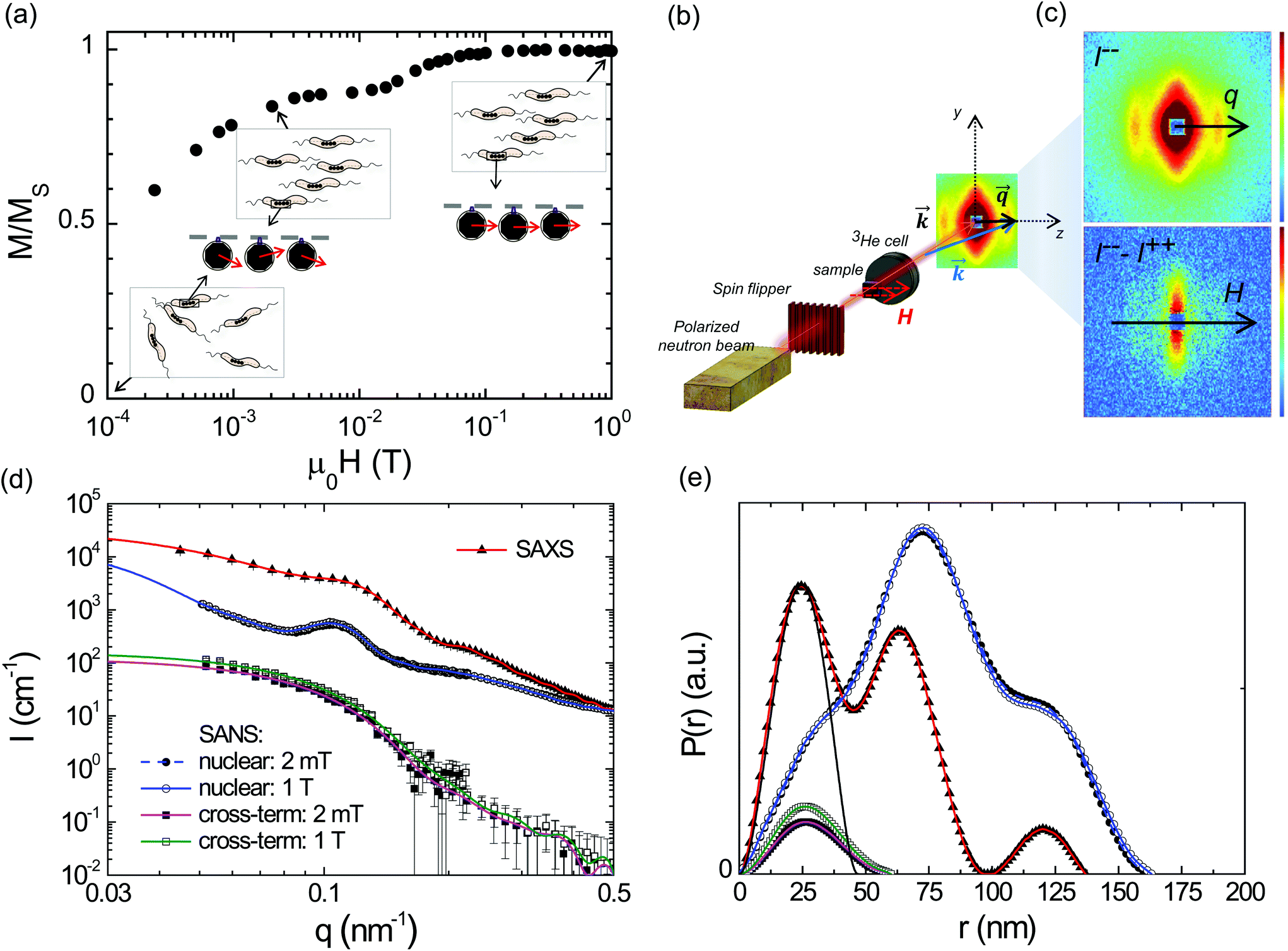

Magnetization and small angle neutron/X-ray scattering (SANS/SAXS) on a bacterial colloid. Fig. 2a shows the RT magnetization curve M(H) of a colloidal dispersion of bacteria (6 × 10¹¹ cells per mL). This curve was measured slowly, leaving two minutes between each data point to assure that thermal equilibrium is achieved at each point. As shown in Fig. 2a, the magnetization increases rapidly with the applied field until it reaches a plateau between 3 mT ≤ μ₀H ≤ 15 mT at a value that is 90% of the saturation value (M = 0.90M_s). Then the magnetization increases again slowly up to saturation. This behavior reveals that there are two different coherent rotations of the magnetization as will be discussed in the following.

Fig. 2 Magnetic state of the colloidal dispersion of bacteria. (a) Magnetization curve of the colloid. The field axis is in logarithmic scale to magnify the low-field region. The sketches display the two-step magnetization process. The experimental data marked with arrows correspond to the points measured by SANS/SAXS (μ₀H = 0 mT;2 mT; and 1 T). (b) Schematic representation of the SANS experiment. The polarized incoming neutron beam can be set to either parallel (+) or antiparallel (−) to the applied field by means of an RF spin flipper. The ³He cell discriminates the polarization of the scattered neutrons (+ or −), hence the recorded intensity is either I⁺⁺ or I⁻⁻, where superindexes refer to the polarization of the incoming/scattered neutrons. (c) 2D SANS scattering patterns for μ₀H = 2 mT. Top: I⁻⁻; bottom: I⁻⁻ − I⁺⁺. (d) 1D scattering intensities measured by SAXS in zero field (radial average, offset by scale factor 100) and the field dependent nuclear scattering intensities I_nuc(q) (offset by scale factor 10) as well as the cross-terms I_cross(q) determined by polarized SANS. The lines are the corresponding fits by an indirect Fourier transform. (e) Pair distance distribution functions P(r) determined by an indirect Fourier transform of the 1D scattering intensities from (d). The black line is the P(r) of a homogeneous sphere with diameter D_SAS = 48 nm. The distribution function determined by SAXS is offset by arbitrary scaling factors.

The magnetic properties of the bacterial colloid have been further investigated via small angle X-ray scattering (SAXS) and polarized small angle neutron scattering (SANS). In a SAXS/SANS experiment the X-ray/neutron beam hits the sample and the scattered beam impacts on a 2D detector perpendicular to the incoming beam (Fig. 2b). The intensity I as a function of the scattering vector gives pure structural (I_nuc(q)) information from SAXS/SANS experiments, or, additionally, magnetic (I_cross(q)) information for SANS depending on the magnetic field on the sample and the polarization of the incoming and scattered neutron beam (Fig. 2c). I_nuc(q) and I_cross(q) are extracted from the 2D scattering patterns (Fig. 2c) as explained in the Methods section.

Fig. 2d shows the radially averaged 1D SAXS intensity I(q) of the colloidal dispersion measured in zero field. An indirect Fourier transform of I(q) results in the pair distance distribution function P(r) as displayed in Fig. 2e. The extracted distribution function exhibits three distinct peaks. The first peak has its maximum at about 25 nm and is nearly bell-shaped. The comparison of this peak with the pair distance distribution function of a homogeneous sphere with diameter D_SAS = 48 nm shows qualitatively very good agreement. Hence, we surmise that the first peak corresponds to the nuclear scattering of the individual magnetosome of an average size of about 48 nm. This particle size is considerably larger than the one obtained by ECT (≈40 nm). The reason for this difference is that ECT is only sensitive to the core of the magnetosome (the magnetic nanoparticle), while the small angle scattering (SAS) techniques are sensitive to both the core and the surrounding lipid bilayer membrane. In particular for neutrons, the scattering cross section of H is very large, which means that organic materials with many H-atoms (such as the lipid membrane in our case) can generate large scattering signals.²⁹ Considering a membrane thickness of ≈4 nm, the core diameter obtained by SANS is 48 − 8 = 40 nm, in agreement with the value obtained from ECT. The maxima of the second and third peaks of the distribution function are at about 75 and 125 nm, and both peaks are also nearly bell-shaped. The positions of the peaks agree well with the expected positions of the center of mass of the next neighbors in a chain-like structure of D_SAS = 48 nm sized particles with a center-to-center distance of d ≈ 50 nm, close to the d ≈ 60 nm distance measured by ECT.

Fig. 2d additionally shows the structural 1D SANS intensities I_nuc(q) detected for field strengths of μ₀H = 2 mT and 1 T applied perpendicularly to the neutron beam. Both I_nuc(q)'s are virtually identical, which means that already at 2 mT the bacteria are fully aligned in the field direction. Consequently an indirect Fourier transform of both nuclear scattering intensities results in superimposed pair distance distribution functions, whose second peak (r ∼ 75 nm) is about twice the height of the first peak (Fig. 2e). This verifies that the bacteria align with the chain axis parallel to the field, considering that within the chain each particle is surrounded on average by two neighbors and thus the probability to find a scatterer at this position is two times the probability to find a scatterer within the primary particle (first peak). To investigate if structural alignment equals magnetic saturation the cross-terms I_cross(q) were analyzed.

The two cross-terms I_cross(q) detected at 2 mT and 1 T display the same functional form (Fig. 2d) and accordingly the extracted distribution functions are qualitatively similar (Fig. 2e). The observation of only one peak can be explained by the fact that the cross terms depict the correlation between nuclear scattering length density and magnetization M_z(r) along the axis perpendicular to the applied field. In all cases the shape of the distribution function is comparable to the distribution function of a single sphere with a homogeneous scattering length density. This verifies that the particles are homogeneously magnetized (i.e. M_z(r) = M_z) and thus can be regarded as single-domain particles. However, the absolute values of P(r) detected at 2 mT are over the whole r-range systematically reduced by a factor of 0.83 compared to 1 T. Assuming that at μ₀H = 1 T the system is saturated in field direction (i.e. M_z = M_s), this means that at 2 mT the magnetization in field direction amounts to M_z = 0.83M_s and that the magnetic saturation is achieved by a coherent rotation of the spins within the individual nanoparticles towards the field direction. These two processes (chain alignment followed by a coherent rotation of the magnetosome spins) explain the isothermal magnetization measurement of the colloid shown in Fig. 2a. In the latter, in agreement with the SANS result, at 2 mT M_z = 0.83M_s, and the coherent rotation of magnetosome spins would start at ≈15 mT, where M_z = 0.9M_s corresponds to a misalignment of the magnetic moment with the chain axis of θ ≈ 25°, where M_z = M_s cos θ.

Magnetometry on 2D and 3D bacterial arrangements. Macroscopic hysteresis loops of M. gryphiswaldense cells have been measured by SQUID and VSM magnetometry. 3D arrangements of aligned bacteria have been obtained by pouring the cells under an applied ‘aligning’ uniform magnetic field into liquid agar that hardens upon cooling. Similarly, 2D arrangements of aligned bacteria have been obtained by depositing the cells onto a Si substrate under . A TEM image of aligned M. gryphiswaldense cells deposited onto a Si substrate is shown in the ESI.† The samples of randomly arranged bacteria have also been prepared in both the 3D and 2D configurations.

The hysteresis loops of randomly arranged and oriented bacteria are shown in Fig. 3a and b, respectively. The hysteresis loops of oriented bacteria have been measured at different angles with respect to between 0° and 90° in steps of 20 degrees for 3D arrangement and at discrete angles, 0°, 45° and 90°, for 2D arrangement. These measurements evidence that bacteria are highly anisotropic magnetic objects, since their hysteresis loops depend strongly on the direction of the applied field. This is not surprising, as one would expect that magnetosome chains behaved as a good compass, with a single magnetic easy axis oriented along the chain axis, which, as noted previously, is coincident with one of the magnetosome 〈111〉 crystallographic axes. However, as previously observed in Magnetospirillum magneticum AMB-1,³⁰ the hysteresis loops of 3D and 2D bacterial arrangements do not correspond to those expected for a uniaxial Stoner–Wohlfarth model³¹ along the chain, since the hysteresis loop perpendicular to the chain axis is not anhysteretic as expected. This could be attributed to the misalignment of the magnetic moment already detected by SANS measurements.

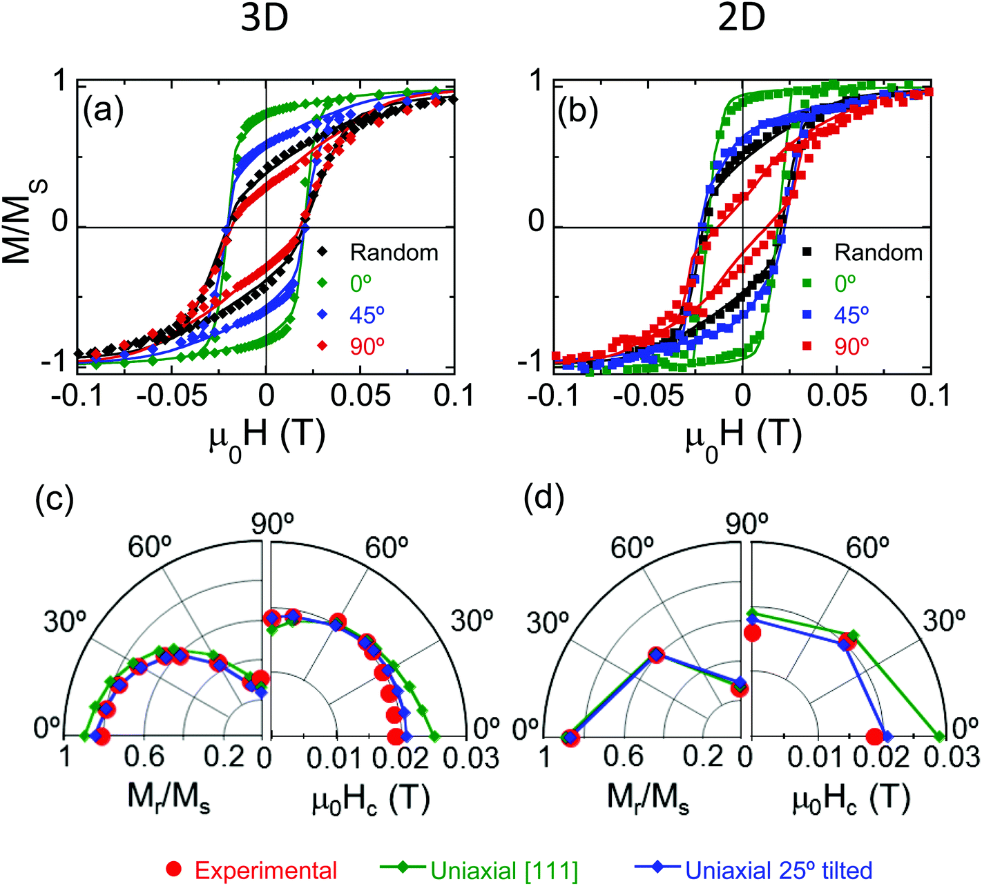Fig. 3 Hysteresis loops of oriented bacteria under an applied field in (a) 3D and (b) 2D arrangements forming 0°, 45°, and 90° with the aligning field , together with the hysteresis loops of randomly arranged bacteria. The continuous line is the fit to the magnetic model explained in the text. (c) and (d) polar plots of the coercivity and reduced remanent magnetization at different orientation angles of the chain axis with in the 3D (c) and 2D (d) arrangements. The experimental points are compared to the results of two simulations in which the uniaxial easy axis û_uni is either parallel (green) or tilted 25° (blue) with the chain axis.

More information on the magnetism of magnetosome chains has been gathered from the theoretical modelling of the hysteresis loops. Previous studies on M. gryphiswaldense show that the magnetic anisotropy of magnetosome chains can be described as a superposition of the cubic magnetocrystalline anisotropy of magnetite, with four equivalent easy axes directed along the 〈111〉 crystallographic directions, and a uniaxial shape anisotropy directed along the chain axis (thus parallel to one of the 〈111〉 axes) that originates from intra-chain dipolar interactions and dominates the magnetic response of the chain.^32,33

Following this argumentation, as a first approximation, our approach to simulate theoretically the experimental hysteresis loops consists of considering the magnetosome chain as a collection of independent magnetic dipoles, where the equilibrium orientation of each magnetic moment is obtained by minimizing the single dipole energy density E, calculated as the sum of three contributions: (i) cubic magnetocrystalline energy of magnetite with anisotropy constant K_c, (ii) uniaxial anisotropy energy along the chain axis ([111] direction defined as û_uni = û₁₁₁ in Fig. 1d) with anisotropy constant K_uni, and (iii) Zeeman energy in an external magnetic field :

E = E_cubic + K_uni[1 − (û_uni·û_m)²] − μ₀MH(û_H·û_m) (1)

where û_m and û_H represent the particle magnetization and external magnetic field unit vectors, respectively. The azimuthal angle can be any between 0° and 360° either because individual dipoles are actually free to be rotated along the chain axis or because whole bacteria themselves can be found at any azimuthal orientations relative to the aligning field due to the sample preparation. The hysteresis loops have then been calculated following a dynamical approach in which the single domain magnetization can switch between the available energy minima states at a rate determined by a Boltzmann factor^34,35 that depends on the energy barriers between such minima. More details are given in the ESI.†

Misalignments of the chains with respect to the aligning field occurring during sample preparation and detected by SANS experiments have been considered by including a Gaussian angular distribution of the chain axes. We have tested three angular distributions around the chain axis: 15°, 25°, and 35°, in agreement with misalignment values reported previously.^28,30 The data used for the simulations are the magnetocrystalline anisotropy constant (K_c = −11 kJ m⁻³) and magnetization (M_s = 48 × 10⁴ A m⁻¹) of magnetite and an effective uniaxial anisotropy constant along the chain axis K_uni = 12 kJ m⁻³ to account for both shape and magnetic interaction anisotropies. Even though the simulations are good enough at the perpendicular orientation, i.e., with the applied magnetic field perpendicular to the bacterial chain axis, they clearly deviate at smaller angles as shown in the polar representation in Fig. 3c, where the experimental and calculated reduced remanent magnetization and coercivity of bacteria in 2D and 3D arrangements are plotted for different orientation angles between 0° and 90°.

Since the misalignment of the bacteria due to sample preparation does not reproduce the hysteresis loops, we have tried a different approach in which we have considered that there is a tilting of the magnetization with respect to the chain axis inherent to the magnetosome. This approach allows the accurate reproduction of the experimental hysteresis loops for both 2D and 3D arrangements by setting the uniaxial easy axis û_uni at 25° with the chain axis in eqn (1), in the plane containing the chain axis ([111]) and the [100] directions. By setting this angle, the effective easy axis, and as a consequence the equilibrium magnetic moment, is found to lie 20° out of the chain axis, in close agreement with the 25° tilting observed in the previous SANS analysis of the colloid. Note that there is a good resemblance with experiment even for an angular dispersion as small as 15° (Fig. 3a and b). We used the same data for the simulations of the hysteresis loops at all orientation angles and for both 3D and 2D arrangements, K_c = −11 kJ m⁻³, M_s = 48 × 10⁴ A m⁻¹ and K_uni = 12 kJ m⁻³. The resemblance with experiment is more evident in the polar plots of the reduced remanent magnetization and coercivity shown in Fig. 3c.

The tilting of the magnetosome magnetization with respect to the chain axis is attributed to the competition between the shape anisotropy of the magnetosome, which presents a well faceted morphology as shown in Fig. 1c, and the magnetic interactions trying to align the magnetic dipoles along the [111] direction parallel to the chain axis. In fact, electron holography experiments on individual magnetosomes from Magnetovibrio blakemorei MV-1 clearly show that the magnetization direction of the particle is tilted with respect to the [111] crystallographic direction towards a long dimension of the particle, consistent with shape anisotropy dominating the magnetic state of the crystal.³⁶

X-ray photoemission electron microscopy (XPEEM) on extracted magnetosomes. Previous magnetic results are supported by X-ray photoemission electron microscopy (XPEEM).³⁷ Unlike the macroscopic SQUID and VSM measurements above, which provide an average measurement of the whole sample, XPEEM is an element-specific and spatially-resolved technique that by using X-ray magnetic circular dichroism (XMCD) as a magnetic contrast mechanism, allows obtaining element-specific magnetic hysteresis loops of selected sample areas with a resolution down to 30 nm.³⁷

XPEEM measurements have been performed at room temperature on extracted magnetosomes due to the high absorbing power of the whole bacteria. Magnetosomes were deposited onto a conductive Si substrate either randomly (Fig. 4c) or oriented along an aligning field (Fig. 4d). As expected for magnetite, the Fe L₃ XMCD signal shows three peaks (Fig. 4b): two minima at 707.4 eV and 709.6 eV and a maximum at 708.6 eV. The two minima correspond to the Fe²⁺ and Fe³⁺ ions occupying tetrahedral sites, and the maximum corresponds to the Fe³⁺ ions occupying octahedral sites. The magnetic contrast images were recorded at the Fe L₃ resonance energy (709.6 eV) of magnetite. The set of magnetic images displayed in Fig. 4c and d show the space-resolved dichroic images obtained at different values of an in-plane magnetic field. The dichroic signal yields the magnetic moment, so that the hysteresis loops of selected areas of the magnetic images (enclosed in rectangles in Fig. 4c and d) have been obtained by plotting the corresponding dichroic signal as a function of the applied magnetic field (Fig. 4a).

Fig. 4 (a) X-ray photoemission electron microscopy (XPEEM) hysteresis loops of the regions enclosed in the rectangles marked in the images in (c) and (d), corresponding to chain sections which are either randomly arranged or forming 0° (green), 60° (blue), and 90° (red) with the applied field. The continuous line is the fit to the magnetic model explained in the text. (b) X-ray absorption spectra (XAS) of the chain parallel to the applied field (green rectangle in c) with the incoming beam right-polarized (σ⁺) and left-polarized (σ⁻). Computing σ⁺ − σ⁻ gives the XMCD signal below. (c) XPEEM images as a function of the applied field of randomly arranged magnetosomes and (d) oriented magnetosomes deposited under . In (d) the SEM image of the chain is shown together with the XPEEM image.

The hysteresis loops of the randomly deposited magnetosomes enclosed in the region marked with the black rectangle in Fig. 4c and of a chain parallel to the applied field, marked with the green rectangle in Fig. 4c, are shown in Fig. 4a.

Magnetosomes deposited under an applied aligning field form longer chains. The XPEEM image together with the SEM image of one of these chains is shown in Fig. 4d. This chain is clearly not a straight line but is rather a zigzag, formed by segments oriented at different angles with the applied field. Two of these segments, enclosed in blue rectangles in Fig. 4d, form 60° with the applied field, and another two segments, in red rectangles, form 90°. The corresponding hysteresis loops are shown in Fig. 4a.

As shown in Fig. 4a, the experimental XPEEM loops can be accurately simulated to the theoretical model developed previously for the 3D and 2D chain arrangements (eqn (1)) with a smaller tilting angle of the effective easy axis (15°) and a larger anisotropy constant K_uni = 16 kJ m⁻³ as compared to the SQUID loops (K_uni = 12 kJ m⁻³). This is attributed to the larger distance between magnetosomes in chains inside the bacteria (d = 60 nm) than in chains of extracted magnetosomes (d = 50 nm). Indeed, for a 40 nm sized particle, the dipole pair potential energy is given by ∼μ₀m²/4πd³ = 0.75 eV (m = M_sV being the particle magnetic moment and d = 60 nm), while for the chains of extracted magnetosomes the dipolar energy from the neighbors at d = 50 nm would increase up to ∼1.35 eV.

Equilibrium configuration of the chain

Following the results gathered from the magnetic analysis, here we will assess the impact on the magnetosome chain configuration of the tilting of the magnetosome magnetization with respect to the chain axis, where the latter, as noted above, is defined as the [111] crystallographic direction along which magnetosomes align in the chain (Fig. 5).

Fig. 5 Equilibrium configuration of the magnetosome chain. (a) Schematic representation of two competing mechanisms: magnetic force pushing to align magnetosome magnetic moments along the stray field lines from neighboring particles, and lipid/protein-based mechanism modeled as an elastic recovery force acting perpendicularly to the chain axis, where the chain axis is the [111] crystallographic direction along which magnetosomes align, as highlighted in the figure. (b) Experimental reconstructions obtained from ECT imaging of the magnetosome chains shown in Fig. 1a and b. A zoom-in of the first magnetosome chain reconstruction highlights the deviation from a straight line. (c) Two stable solutions for the chain patterns obtained as explained in the text. A potential filament has been drawn as a guide for the eye. A video of the experimental reconstruction of the chain on the left (chain (a) in Fig. 1) together with the corresponding simulated chain viewed from different perspectives can be found in the ESI (movie S3†). (d) Schematic representation of the magnetic dipoles and the three independent variables used in the simulation: radial (ρ) and azimuthal (ϕ) coordinates for the magnetosome positions, and azimuthal orientation (φ) of the magnetic dipoles. θ is the polar angle of the magnetic dipoles, fixed to 20°.

With this aim, we have developed an approach to explain the shape of the magnetosome chains that consists of quantifying the total energy of the chain by including the magnetostatic interactions between nanoparticles, and the contribution of the lipid/protein-based architecture embedding the magnetosome chain, modeled as a spring-like elastic energy. We focus on the stable geometry of chain arrangements and assume that close loop configurations such as rings or 3D clusters are avoided by the cytoskeleton inside bacteria. The same approach has been used by other authors,^22,38 but in the present case, as proposed previously, the magnetization of each magnetosome is tilted 20° out of the chain axis.

Here we will summarize the main steps followed to calculate the total energy of the chain, but a detailed description can be found in the ESI.†Fig. 5a shows a section of a magnetosome chain composed of three magnetosomes. The particle in the centre is subjected to the stray magnetic field produced by the two neighbors (the dotted red lines in Fig. 5a represent the stray field produced by the particle at the bottom). We implicitly assume that the local torque that tends to align neighboring dipoles is counter-balanced by the cytoskeleton, since cryotomography and TEM images reflect that the hexagonal faces are face to face.^27,28 The particle in the middle will tend to align its magnetization along the stray field lines and will undergo a magnetic force that compels it to shift towards the direction of its own magnetic moment. The magnetostatic energy associated with the magnetic force on magnetosomes is then implemented as the sum of the dipolar pair potential energies between nearest neighboring particles.

On the other hand, magnetite crystals are embedded in a lipid/protein-based architecture composed, among others, of the magnetosome membranes, the cytoskeletal filaments, and the proteins connecting the magnetosome membranes with the cytoskeleton. The contribution to the total chain energy of this lipid/protein-based architecture has been modeled based on two simplifying assumptions: firstly, that the distance between particles, d, is fixed, so that chains can bend or twist but cannot stretch; and secondly, that the net force on the magnetosomes can be ascribed to an elastic recovery force with elastic constant k acting perpendicularly to the chain axis, as shown in Fig. 5a.

The most stable chain configurations have then been predicted by minimizing the total energy of the chain considering three independent variables per particle, namely the radial (ρ) and azimuthal (ϕ) coordinates for the magnetosome positions, and azimuthal orientation (φ) of the magnetic dipoles (see sketch in Fig. 5d). The results have then been compared to the 3D reconstructions obtained from the chains imaged by ECT (Fig. 5b).

Considering a particle diameter D = 40 nm, distance between them d = 60 nm, and k = 0.1 × 10^–3 N m⁻¹, two stable solutions give the patterns shown in Fig. 5c, in excellent match with the two experimental chain reconstructions shown in Fig. 5b. They are helical-like shaped chains with slowly bending axes and a different pitch, given by ≈2L/n, L = Nd being the chain length, N the number of magnetosomes per chain, and n = 1 and 2, respectively. The energy difference between the two chain shapes is less than 1% of the total energy, hence they are approximately equally stable. The agreement between the simulated and the experimental chains is even more explicit in a video of images of both chains taken from different perspectives shown in the ESI (movie S3†).

A zoom-in of a section of one of the simulated chains shows the magnetosome dipole moments. The azimuthal increment of the individual dipole orientations (Δφ) between consecutive positions along the chain increases with n approximately as:

where N is the number of magnetosomes per chain (N = 15 and 22 in the two examples shown). Consequently, the component of the chain magnetization vector (the vector sum of the magnetic moment of each magnetosome) perpendicular to the chain axis cancels out, so that the chain magnetization lies along the chain axis. Also note that when magnetic dipoles are projected in a 2D view of the chain, apparent tilting between consecutive dipoles is no more than 7° (see Fig. 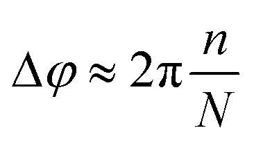4 in the ESI†), which is compatible with projected electron holography images.²

The role of k in chain geometry is to scale up or down the radial positions of magnetosomes along the chain, so that larger k favours configurations approaching straight lines. In our case, k = 0.1 × 10^–3 N m⁻¹ results in assembling forces of the order of 0.6 pN for radial displacements of ≈10 nm as obtained from the simulations, similar to the force generated by the actin filament,³⁹ and far below recent estimations of the fracture limit of the actin-based scaffolding filaments (≈30 pN) as reported by Körnig et al.⁴⁰

On the basis of our results, a mechanism of chain formation is proposed. Our findings reveal that the chain shape is mostly driven by passive spontaneous magnetostatic effects triggered by the intrinsic anisotropy of magnetosomes, ultimately defined by their morphology. The magnetosome morphology is regulated during the biomineralization process. This is a genetically controlled process which involves a specific set of about 30 mam (magnetosome membrane) and mms (magnetic particle-membrane specific) genes.⁴ The product of the mamJ gene is an acidic protein that connects the magnetosome membrane to the filament. The deletion of mamJ results in bacteria that produce magnetosomes arranged in compact three-dimensional clusters instead of arranged in chains.²⁶ The fact that they form clusters and not closed rings is consistent with our conclusions, namely the tilting of the magnetosome magnetic moment with respect to the chain [111] axis, since according to previous studies, more than four magnetosomes tend to form closed rings when their magnetic moment is parallel to the [111] axis.³⁸ In the same way, when depositing the magnetosomes onto a 2D surface, magnetosomes tend to self-assemble in a close-packing configuration,⁴¹ and the tilting could also be behind the zigzag configuration of the chains observed by SEM in oriented magnetosomes. But, why would this helical-like shape benefit the bacteria? M. gryphiswaldense are long cells, easily reaching several microns long. They need a high magnetic torque to overcome the drag forces and orientate along the Earth's magnetic field. As a consequence, their magnetosome chain needs to be long to maximize the chain net magnetic moment. Indeed, their chain is frequently composed of more than 20 magnetosomes, which brings the total length of the chain to 1.5 μm or more, about 50–60% of the bacterial length. Such an object should necessarily be bent in order to accommodate this spiral-shaped microorganism. Thus a helical-like shape fits better, but it only changes slightly the total magnetic moment, hence hardly affecting the magnetic orientation. A genetic control of the magnetosome shape towards an energetically optimum chain arrangement is also observed in Magnetobacterium bavaricum MYR-1, a species which synthesize bullet-shaped magnetosomes arranged into bundles of magnetosome chains. The magnetosome magnetization within MYR-1 magnetosomes is parallel to the chain axis, which coincides with the long axis of the magnetosomes. Unexpectedly, the latter is parallel to the [100] crystallographic axis, a magnetically hard axis in magnetite, rather than along the [111] magnetocrystalline easy axis, due to compromise effects of shape anisotropy and intra-chain and intra-bundle interactions.⁴²

In summary, our finding sheds light on the understanding of the magnetosome chain assembly during the biomineralization process of MTB, which may influence their potential future applications as biological micro-robots. Indeed, one of the major technical issues in the development of interventional platforms for guiding drug-loaded MTB is the directional magnetic field strength that needs to be produced at the human scale to induce sufficient directional torque on the chain of magnetosomes. A good knowledge of the magnetic configuration of the magnetosome chain will lead to more efficient and less costly drug-delivery platforms that may benefit a larger population.

Methods

Magnetotactic bacteria culture and magnetosome isolation

Magnetospirillum gryphiswaldense MSR-1 (DMSZ 6631) was grown at 28 °C without shaking in an iron rich medium.⁴³ After 96 h-incubation, when bacteria present well-formed magnetosome chains, the cells were fixed with 2% glutaraldehyde, harvested by centrifugation, washed three times and finally concentrated up to 10⁹–10¹¹ cells per mL in ultrapure water. Magnetosomes were isolated according to the protocol described by Grünberg et al.⁴⁴ with minor modifications. The cells were collected by centrifugation, suspended in 20 mM HEPES–4 mM EDTA (pH = 7.4), and disrupted using a French press (1.4 kbar). Then, the magnetosomes were collected from the supernatant by magnetic separation and rinsed 10 times with 10 mM Hepes–200 mM NaCl (pH = 7.4). Finally, the isolated magnetosomes were suspended in ultrapure water reaching a concentration of 20 μg mL⁻¹.

Electron cryotomography (ECT)

Sample preparation for cryotomography was as follows: a 10 μl volume of fixed and washed M. gryphiswaldense cells (10⁹ cells per mL) was mixed with a 3 μl volume of 10 nm Au nano-particles (Aurion®BSA gold tracer 10 nm) (used as fiducial markers). This mixture is frozen-hydrated following standard methods using a Vitrobot Mark III (FEI Inc., Eindhoven, The Netherlands). In brief, a grid is placed in the controlled environment of the Vitrobot chamber, which is at 4 °C and at a relative humidity of 95%. An aliquot (4 μl) of the sample is applied to a glow-discharged grid. After 1 min incubation most of the drop is removed by blotting with two filter papers, to produce a thin liquid film, and rapidly plunged into liquid ethane (91 K), previously cooled by liquid nitrogen. Vitrified grids are stored under liquid nitrogen until cryo-TEM data collection. For cryo-tomographic tilt series acquisition, vitrified grids were cryo-transferred into a 914 high tilt tomography cryo-holder (Gatan Inc., Warrendale, PA, USA), which is inserted in a JEM-2000FS/CR field emission gun transmission electron microscope (Jeol, Europe, Croissy-sur-Seine, France) operated at 200 kV. Grids are kept around 103 K in the high vacuum of the microscope column containing the sample embedded in a thin layer of glass-like vitreous ice, in a near native-state. Different single-axis tilt series were collected under low-dose conditions on an UltraScan 4000, 4k × 4k CCD camera (Gatan Inc., Pleasanton, CA, USA), over a tilt range of ±64° with 1.5° increments and at underfocus values ranging from 5 to 8 μm, using the semi-automatic data acquisition software SerialEM.⁴⁵ Tilt-series were collected at a nominal magnification of 25 000× and a binning factor of 2 (2048 × 2048 pixel micrographs), thus producing a pixel size of 0.95 nm. The in-column omega energy filter helped to record images with an improved signal-to-noise-ratio by zero-loss filtering with an energy window of 60 eV centered at the zero-loss peak. CCD images in each tilt-series were acquired at the same underfocus value and under the same low-dose conditions. The maximum total dose used for a tilt-series was 90 electrons per Ų consisting of about 1–2 electrons per Ų for each digital image.

For the alignment and 3D reconstruction of the tilt-series, we used IMOD software.⁴⁶ We employed the Au fiducial markers during the alignment process, and 3D reconstruction was carried out by weight back-projection followed by a reconstruction algorithm named the Simultaneous Iterative Reconstruction Technique (SIRT). The resulting tomograms were visualized with ImageJ⁴⁷ as a sequence of cross sectional slices in different plane orientations. Tomograms were processed using a median filter and visualized as 3D electron density maps using UCSF Chimera⁴⁸ software.

Scanning electron microscopy (SEM)

SEM imaging was performed on the two magnetosome samples measured in XPEEM (magnetically oriented and randomly arranged). SEM images were collected at 10 kV with a JEOL JSM-7000F equipped with secondary and retro dispersive electron detectors.

Magnetic measurements

Magnetic measurements on bacteria forming 2D and 3D arrangements were performed on a superconducting quantum interference device magnetometer (SQUID, Quantum Design MPMS-7) in DC mode and on a vibrating sample magnetometer (VSM). Isothermal magnetization loops were recorded between ±1 T at 300 K.

The 2D bacterial configurations were prepared by depositing five 5 μL drops of the bacterial suspension (10⁹ cells per mL) by the drop coating method^41,49 onto a Si substrate. For the oriented bacteria, the deposition was done under an external applied magnetic field of 0.5 T. To obtain homogeneous samples, infrared radiation was used during the deposition aimed at accelerating the drying and minimising the surface tension. The resulting samples were finally oriented at different angles with respect to the applied magnetic field.

The 3D bacterial configurations were prepared by resuspending 250 μl of a bacterial colloid (10¹¹ cells per mL) in 750 μl of an agar solution (2% agar and 98% water) at 60 °C to maintain the solution in a liquid state. To align the bacteria, a uniform magnetic field of 1 T was applied. After 3 minutes, the field was turned off, and the sample was cooled using liquid nitrogen until the temperature reached around 0 °C. This caused the agar to solidify, trapping the bacteria, and keeping this solid state at room temperature.

Small angle neutron scattering (SANS) and small angle X-ray scattering (SAXS)

SANS/SAXS experiments were performed on a highly concentrated bacterial colloid (6 × 10¹¹ cells per mL) suspended in ultrapure water. The magnetization curve of the colloid was measured on a vibrating sample magnetometer up to an applied field of 1 T, leaving two minutes between each measurement to assure that thermal equilibrium was achieved at each point.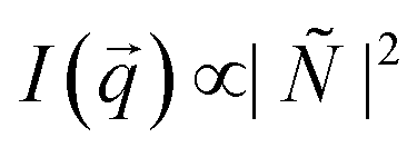

Small angle X-ray scattering (SAXS) experiments. The SAXS data were collected in a Xenocs Nano-InXider, using a 40 μm microfocus Cu anode as an X-ray source and a multilayer monochromator to collect only the Cu-Kα radiation. The detector (a Pilatus 3) is at 938 mm from the sample, spans an area of 83.8 × 33.5 μm² and a pixel size of 172 × 172 μm². The colloidal dispersion was filled into a quartz glass capillary and was measured in the absence of an externally applied magnetic field. Via SAXS exclusively the nuclear scattering intensity is determined, with being the scattering wave vector and 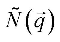being the Fourier transform of the nuclear scattering length density . To analyze the data we performed an indirect Fourier transform⁵⁰ of the radially averaged 1D intensity I(q) to extract the pair distance distribution function P(r). The real space function P(r) provides direct information about the distances between scatterers from the scattering sample⁵¹ and hence contains information about the average particle geometry as well as correlations between neighboring particles. For the indirect Fourier transform we used an approach based on ref. 52 and computational details can be found in ref. 53.

Polarized small angle neutron scattering (SANS) experiments. The SANS instrument D33 at the Institut Laue Langevin (ILL, Grenoble, France)^54,55 was employed to carry out a longitudinal neutron-spin analysis (POLARIS).⁵⁶ A homogeneous magnetic field was applied perpendicular to the neutron beam with field amplitudes of μ₀H = 2 mT and 1 T. The mean wavelength of the neutrons was λ = 0.6 nm, with a wavelength spread of Δλ/λ = 10%. The scattering intensities were measured at two different detector distances (3 m and 13.4 m) giving a q-range of about 0.05–0.5 nm⁻¹.

The application of the POLARIS mode enabled us to detect the non-spin flip (nsf) intensities 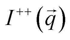, , where the superscripts indicate the polarization of the incoming neutron beam and the scattered neutrons with regard to the applied field direction, respectively (“+”: parallel, “−”: antiparallel). Defining x as the direction of the neutron beam and z as the direction of the applied magnetic field at the sample position the nsf intensities can be written as:⁵⁶

Here, Θ is the angle between the scattering vector and the magnetic field and the terms represent the Fourier transforms of the magnetization in the y, z direction. The superscript * indicates the complex-conjugated quantities and the constant b_H = 2.7 × 10⁻¹⁵ m/μ_B⁻¹, with μ_B being the Bohr magneton. To investigate the alignment of the bacteria in field direction we analyzed the 1D nuclear cross sections I_nuc(q)∝|Ñ|² and the 1D nuclear magnetic cross-terms . The purely nuclear scattering intensities were determined by integration of the nsf intensities in 10° sectors around Θ = 0° (, eqn (3)) and the cross terms I_cross(q) by integration of in 10° sectors around Θ = 90° (, eqn (3)). The difference between the two nsf cross sections yields information on the polarization-dependent nuclear-magnetic terms. This difference allows one to highlight weak magnetic contributions relative to strong nuclear scattering (or vice versa). From the determined cross sections we extracted the underlying pair distance distribution functions in the same manner as for SAXS. In H₂O, there is a contrast match of bacteria in the dispersion, such that only the magnetosomes and their arrangement are probed by SANS.

X-ray photoelectron emission microscopy (XPEEM)

For the X-ray photoemission electron microscopy (XPEEM) experiments isolated magnetosomes extracted from the bacteria were employed. Two different samples were prepared. The first one consists of randomly arranged magnetosomes prepared by the deposition of a 5 μL drop of the magnetosome suspension onto a conductive Si substrate. The drop was dried under infrared radiation. The second sample consists of magnetically oriented magnetosomes. In this case, the drop was dried under an external magnetic field of 0.5 T and infrared radiation. The Si substrate was marked with an Au reticule to allow subsequent match by scanning electron microscopy (SEM) of the chains imaged by XPEEM.

Magnetic imaging of the isolated magnetosomes was performed at room temperature by means of photoelectron emission microscopy (PEEM) by using X-ray magnetic circular dichroism (XMCD) as a magnetic contrast mechanism. Measurements were carried out at the UE49_PGM SPEEM beamline at Helmholtz-Zentrum Berlin. A magnetic solenoid attached to the sample holder allowed the application of an in-plane pulsed magnetic field ranging ±0.1 T to saturate the sample. During imaging the magnetic field range was restricted to ±27.5 mT. The incoming photon energy was tuned to the Fe L₃ resonance (709.6 eV) to obtain element specific XMCD images of the magnetosomes as a function of the applied magnetic field. At each field a sequence of images was acquired with incoming circular polarized radiation (90% of circular photon polarization) with left (σ⁻) and right helicity (σ⁺), respectively. To improve statistics we acquired up to 400 images per helicity and field (3 s of exposure time). After normalization to a bright-field image, the sequence was drift-corrected, and frames recorded with the same helicity were averaged.

XMCD images. Displayed XMCD images were obtained by computing XMCD = ((σ⁺ − σ⁻)/(σ⁺ + σ⁻)). Due to the low signal, the XMCD strength at the regions of interest was comparable to the noise level at nearby regions with no magnetic particles. In order to enhance the magnetic contrast, for visualization purposes only, the XMCD images have been multiplied by the X-ray absorption image, i.e. XAS = σ⁺ + σ⁻ after background subtraction.

Space-resolved magnetic hysteresis loops. The data analysis allowed obtaining the magnetic hysteresis loop of any region within the field of view. In order to obtain the magnetic hysteresis (XMCD vs. magnetic field) of a selected magnetosome region we computed the intensity as a function of field and helicity (σ⁺ and σ⁻) on the selected area. A local background subtraction was performed by calculating the intensity variation observed within nearby regions with no magnetic particles (substrate). The XMCD is then calculated as the difference between background corrected σ⁺ and σ⁻ divided by their sum, i.e. XMCD = (σ⁺ − σ⁻)/(σ⁺ + σ⁻).

Space-resolved XAS and XMCD spectra. For both, left and right helicities of the incoming circular polarized radiation, five stacks of images were obtained as the incoming photon energy crossed the Fe L_3,2 edges. The photon energy was varied between 690 eV and 730 eV in 0.2 eV steps. The total integration time per energy was 2.5 s. After normalization to a bright-field image, the sequence was drift-corrected, and the frames recorded with the same helicity and photon energy were averaged. Computing of local X-ray absorption spectra (XAS) for σ⁺ and σ⁻ allows the calculation of the X-ray magnetic circular dichroism spectrum as σ⁺ − σ⁻ from a selected region.

Author contributions

I. O. and M. F. G. designed research; I. O. and L. M. performed and analyzed SQUID and VSM measurements; L. M., A. G. P., A. M., M. F. G, S. V. and M. A. M. performed XPEEM measurements; L. M., S. V. and A. G. P. analyzed XPEEM data; P. B, L. M., D. A. V. and D. H. performed SAXS/SANS experiments; P. B. analyzed SAXS/SANS data; I. O. conceived the chain configuration model; I. O., L. M., P. B., A. G. P., A. G. A., L. F. B. and M. F. G. discussed the magnetic results; L. M., A. M., M. F. G. and D. G. performed and analyzed the cryotomography imaging; I. O., L. M., P. B., A. G. P. and M. F. G. wrote the paper; all authors checked the manuscript; A. M. and M. F. G. supervised the work.

Conflicts of interest

There are no conflicts to declare.

Acknowledgements

The Spanish Government is acknowledged for funding under projects number MAT2014-55049-C2-R and MAT2017-83631-C3-R. The Basque Government is acknowledged for L.M.'s fellowship (PRE_2015_1_0130) and for funding under project number IT711-13. We also acknowledge funding from the EU through project NanoMag (grant agreement no. 604448). We thank the Institut Laue Langevin for provision of beamtime at the instrument D33 and the Science and Technology Facilities Council (STFC) for access to the SAXS kit at the Materials Characterisation Laboratory. We thank HZB for the allocation of synchrotron radiation beamtime and funding. The authors are grateful to D. Muñoz, D. Gandia and A. Vigilante for preparing the samples for the magnetometry measurements.

References

1. R. Blakemore, Science, 1975, 190, 377.
2. R. E. Dunin-Borkowski, M. R. McCartney, R. B. Frankel, D. A. Bazylinski, M. Posfai and P. R. Buseck, Science, 1998, 282, 1868.
3. D. A. Bazylinski and R. B. Frankel, Nat. Rev. Microbiol., 2004, 2, 217–230.
4. R. Uebe and D. Schüler, Nat. Rev. Microbiol., 2016, 14, 621–637.
5. C. T. Lefevre and D. A. Bazylinski, Microbiol. Mol. Biol. Rev., 2013, 77, 497–526.
6. D. Serantes, K. Simeonidis, M. Angelakeris, O. Chubykalo-Fesenko, M. Marciello, M. Morales, D. Baldomir and C. Martínez-Boubeta, J. Phys. Chem. C, 2014, 118, 5927–5934.
7. O. Felfoul, M. Mohammadi, S. Taherkhani, D. de Lanauze, Y. Zhong Xu, D. Loghin, S. Essa, S. Jancik, D. Houle, M. Lafleur, L. Gaboury, M. Tabrizian, N. Kaou, M. Atkin, T. Vuong, G. Batist, N. Beauchemin, D. Radzioch and S. Martel, Nat. Nanotechnol., 2016, 11, 941–949.
8. D. Ghosh, Y. Lee, S. Thomas, A. G. Kohli, D. S. Yun, A. M. Belcher and K. A. Kelly, Nat. Nanotechnol., 2012, 7, 677–682.
9. E. Alphandéry, S. Faure, O. Seksek, F. Guyot and I. Chebbi, ACS Nano, 2011, 5, 6279–6296.
10. S. R. Mishra, M. D. Dickey, O. D. Velev and J. B. Tracy, Nanoscale, 2016, 8, 1309–1313.
11. X. Jiang, J. Feng, L. Huang, Y. Wu, B. Su, W. Yang, L. Mai and L. Jiang, Adv. Mater., 2016, 28, 6952–6958.
12. X. Kou, X. Fan, R. K. Dumas, Q. Lu, Y. Zhang, H. Zhu, X. Zhang, K. Liu and J. Q. Xiao, Adv. Mater., 2011, 23, 1393–1397.
13. A. Komeili, Annu. Rev. Biochem., 2007, 76, 351–366.
14. D. Faivre and D. Schüler, Chem. Rev., 2008, 108, 4875–4898.
15. A. Komeili, Z. Li, D. K. Newman and G. J. Jensen, Science, 2006, 311, 242–245.
16. R. B. Frankel, G. C. Papaefthymiou, R. P. Blakemore and W. O'Brien, Biochim. Biophys. Acta, 1983, 763, 147–159.
17. M. L. Fdez-Gubieda, A. Muela, J. Alonso, A. García-Prieto, L. Olivi, R. Fernández-Pacheco and J. M. Barandiarán, ACS Nano, 2013, 7, 3297–3305.
18. J. Baumgartner, G. Morin, N. Menguy, T. Perez Gonzalez, M. Widdrat, J. Cosmidis and D. Faivre, Proc. Natl. Acad. Sci. U. S. A., 2013, 1, 1–6.
19. A. Komeili, FEMS Microbiol. Rev., 2012, 36, 232–255.
20. M. Toro-Nahuelpan, F. D. Müller, S. Klumpp, J. M. Plitzko, M. Bramkamp and D. Schüler, BMC Biol., 2016, 1–24.
21. E. Cornejo, P. Subramanian, Z. Li, G. J. Jensen and A. Komeili, mBio, 2016, 7, e01898–e01815.
22. V. P. Shcherbakov, M. Winklhofer, M. Hanzlik and N. Petersen, Eur. Biophys. J., 1997, 26, 319–326.
23. S. Klumpp and D. Faivre, PLoS One, 2012, 7, 1–11.
24. A. G. Meyra, G. J. Zarragoicoechea and V. A. Kuz, Phys. Chem. Chem. Phys., 2016, 18, 12768–12773.
25. E. Katzmann, A. Scheffel, M. Gruska, J. M. Plitzko and D. Schüler, Mol. Microbiol., 2010, 77, 208–224.
26. A. Scheffel, M. Gruska, D. Faivre, A. Linaroudis, J. M. Plitzko and D. Schuler, Nature, 2006, 440, 110–114.
27. S. Mann, R. B. Frankel and R. P. Blakemore, Nature, 1984, 310, 405–407.
28. A. Körnig, M. Winklhofer, J. Baumgartner, T. P. González, P. Fratzl and D. Faivre, Adv. Funct. Mater., 2014, 24, 3926–3932.
29. A. Hoell, A. Wiedenmann, U. Heyen and D. Schüler, Physica B, 2004, 350, 309–313.
30. J. Li, K. Ge, Y. Pan, W. Williams, Q. Liu and H. Qin, Geochem., Geophys., Geosyst., 2013, 14, 3887–3907.
31. E. C. Stoner and E. P. Wohlfarth, Philos. Trans. R. Soc. London, Ser. A, 1948, 240, 599–642.
32. M. Charilaou, M. Winklhofer and A. U. Gehring, J. Appl. Phys., 2011, 109, 1–6.
33. M. Charilaou, K. K. Sahu, D. Faivre, A. Fischer, I. García-Rubio and A. U. Gehring, Appl. Phys. Lett., 2011, 99, 9–11.
34. L. J. Geoghegan, W. T. Coffey and B. Mulligan, Adv. Chem. Phys., 1997, 100, 475–641.
35. J. Carrey, B. Mehdaoui and M. Respaud, J. Appl. Phys., 2011, 109, 083921.
36. J. M. Thomas, E. T. Simpson, T. Kasama and R. E. Dunin-Borkowski, Acc. Chem. Res., 2008, 41, 665–674.
37. F. Kronast and S. Valencia, JLSRF, 2016, A90, 1–6.
38. B. Kiani, D. Faivre and S. Klumpp, New J. Phys., 2015, 17, 43007.
39. M. J. Footer, J. W. J. Kerssemakers, J. A. Theriot and M. Dogterom, Proc. Natl. Acad. Sci. U. S. A., 2007, 104, 2181–2186.
40. A. Körnig, J. Dong, M. Bennet, M. Widdrat, J. Andert, F. D. Müller, D. Schüler, S. Klumpp and D. Faivre, Nano Lett., 2014, 14, 4653–4659.
41. A. M. Huízar-Félix, D. Muñoz, I. Orue, C. Magén, A. Ibarra, J. M. Barandiarán, A. Muela and M. L. Fdez-Gubieda, Appl. Phys. Lett., 2016, 108, 063109.
42. J. Li, Y. Pan, Q. Liu, K. Yu-Zhang, N. Menguy, R. Che, H. Qin, W. Lin, W. Wu, N. Petersen and X. Yang, Earth Planet. Sci. Lett., 2010, 293, 368–376.
43. U. Heyen and D. Schüler, Appl. Microbiol. Biotechnol., 2003, 61, 536–544.
44. K. Grünberg, C. Wawer and B. M. Tebo, Appl. Environ. Microbiol., 2001, 67, 4573–4582.
45. D. N. Mastronarde, J. Struct. Biol., 2005, 152, 36–51.
46. J. R. Kremer, D. N. Mastronarde and J. McIntosh, J. Struct. Biol., 1996, 116, 71–76.
47. J. Schindelin, C. T. Rueden, M. C. Hiner and K. W. Eliceiri, Mol. Reprod. Dev., 2015, 82, 518–529.
48. E. F. Pettersen, T. D. Goddard, C. C. Huang, G. S. Couch, D. M. Greenblatt, E. C. Meng and T. E. Ferrin, J. Comput. Chem., 2004, 25, 1605–1612.
49. H. Gojzewski, M. Makowski, A. Hashim, P. Kopcansky, Z. Tomori and M. Timko, Scanning, 2012, 34, 159–169.
50. O. Glatter, J. Appl. Crystallogr., 1977, 10, 415–421.
51. O. Glatter, J. Appl. Crystallogr., 1979, 12, 166–175.
52. B. Vestergaard and S. Hansen, J. Appl. Crystallogr., 2006, 39, 797–804.
53. P. Bender, L. Bogart, O. Posth, W. Szczerba, S. Rogers, A. Castro, L. Nilsson, L. Zeng, A. Sugunan and J. Sommertune, et al. , Sci. Rep., 2017, 7, 45990.
54. C. D. Dewhurst, I. Grillo, D. Honecker, M. Bonnaud, M. Jacques, C. Amrouni, A. Perillo-Marcone, G. Manzin and R. Cubitt, J. Appl. Crystallogr., 2016, 49, 1–14.
55. P. Bender, L. Fernández Barquín, M. L. Fdez-Gubieda, D. González-Alonso, D. Honecker, L. Marcano and W. Szczerba, Spin correlation in clusters of magnetic nanoparticles, Institut Laue-Langevin (ILL), 2017, DOI: 10.5291/ILL-DATA.5-53-267.
56. D. Honecker, A. Ferdinand, F. Döbrich, C. Dewhurst, A. Wiedenmann, C. Gómez-Polo, K. Suzuki and A. Michels, Eur. Phys. J. B, 2010, 76, 209–213.

---

Footnote

† Electronic supplementary information (ESI) available: TEM image of oriented bacteria, details on the calculation of the hysteresis loops, calculation of the chain energy, and 2D projection of the magnetic dipoles. Movies S1 and S2: Videos of the tomograms of the three chains in Fig. 1a and b viewed as consecutive slices in XY, YZ, and YZ plane orientations, and as an electron density map. Movie S3: Video of the experimental reconstruction of the chain in Fig. 1a (corresponding to n = 1 in Fig. 5b) together with the corresponding simulated chain (Fig. 5c) viewed from different perspectives. See DOI: 10.1039/C7NR08493E

---