
 Open Access Article
 This Open Access Article is licensed under a
 Creative Commons Attribution 3.0 Unported Licence
Can machine learning identify the next high-temperature superconductor? Examining extrapolation performance for materials discovery
Bryce
Meredig
 *a,
Erin
Antono
a,
Carena
Church
a,
Maxwell
Hutchinson
a,
Julia
Ling
a,
Sean
Paradiso
a,
Ben
Blaiszik
bc,
Ian
Foster
bc,
Brenna
Gibbons
d,
Jason
Hattrick-Simpers
e,
Apurva
Mehta
f and
Logan
Ward
bc
*a,
Erin
Antono
a,
Carena
Church
a,
Maxwell
Hutchinson
a,
Julia
Ling
a,
Sean
Paradiso
a,
Ben
Blaiszik
bc,
Ian
Foster
bc,
Brenna
Gibbons
d,
Jason
Hattrick-Simpers
e,
Apurva
Mehta
f and
Logan
Ward
bc
aCitrine Informatics, USA. E-mail: bryce@citrine.io
bUniversity of Chicago, USA
cArgonne National Laboratory, USA
dStanford University, USA
eNational Institute of Standards and Technology, USA
fSLAC National Accelerator Laboratory, USA
First published on 17th August 2018
Abstract
Traditional machine learning (ML) metrics overestimate model performance for materials discovery. We introduce (1) leave-one-cluster-out cross-validation (LOCO CV) and (2) a simple nearest-neighbor benchmark to show that model performance in discovery applications strongly depends on the problem, data sampling, and extrapolation. Our results suggest that ML-guided iterative experimentation may outperform standard high-throughput screening for discovering breakthrough materials like high-Tc superconductors with ML.
Design, System, ApplicationMachine learning (ML) has become a widely-adopted predictive tool for materials design and discovery. Random k-fold cross-validation (CV), the traditional gold-standard approach for evaluating the quality of ML models, is fundamentally mismatched to the nature of materials discovery, and leads to an overly optimistic measure of ML model performance for many discovery problems. To address this challenge, we describe two techniques for contextualizing ML model performance for materials discovery: leave-one-cluster-out (LOCO) CV, and a naïve first-nearest-neighbor baseline model. These tools provide a more comprehensive and realistic picture of ML model performance in materials discovery applications. |
Materials informatics (MI), or the application of data-driven algorithms to materials problems, has grown quickly as a field in recent years.1,2 One common task in materials informatics is the use of machine learning (ML) for the prediction of materials properties. Examples of recent models built with ML include steel fatigue strength,3 small molecule properties calculated from density functional theory,4 thermodynamic stability,5 Gibbs free energies,6 band gaps of inorganic compounds,7 alloy formation enthalpies,8 and grain boundary energies.9 Across all of these applications, a training database of simulated or experimentally-measured materials properties serves as input to a ML algorithm that predictively maps features (i.e., materials descriptors) to target materials properties.
Ideally, the result of training such models would be the experimental realization of new materials with promising properties. The MI community has produced several such success stories, including thermoelectric compounds,10,11 shape-memory alloys,12 superalloys,13 and 3d-printable high-strength aluminum alloys.14 However, in many cases, a model is itself the output of a study, and the question becomes: to what extent could the model be used to drive materials discovery?
Typically, the performance of ML models of materials properties is quantified via cross-validation (CV). CV can be performed either in a single division of the available data into a training set (to build the model) and a test set (to evaluate its performance), or as an ensemble process known as k-fold CV wherein the data are partitioned into k non-overlapping subsets of nearly equal size (folds) and model performance is averaged across each combination of k-1 training folds and one test fold. Leave-one-out cross-validation (LOOCV) is the limit where k is the number of total examples in the dataset. Table 1 summarizes some examples of model performance statistics as reported in the aforementioned studies (some studies involved testing multiple algorithms across multiple properties).
| Material class | Property | ML technique | CV type | Model performance metric | Ref. |
|---|---|---|---|---|---|
| Steel | Fatigue strength | Multivariate polynomial regression | Leave-one-out CV | R 2 = 0.9801 | 3 |
| Organic small molecules | Norm of dipole moment | Graph convolutions | Overall 90% train/10% test, with reported test error averaged across 10 different models built on subsets of training data | MAE = 0.101 Debye (chemical accuracy target: 0.10 Debye) | 4 |
| Polymers | Electronic dielectric constant | Kernel ridge regression | 81% train/19% test | R 2 = 0.96 | 16 |
| Inorganic compounds | Formation energy | Rotation forest | 32% train/68% test | R 2 = 0.93 | 5 |
| Inorganic compounds | Vibrational free energy | Random forest or support vector machine | 10 averaged k-fold CV runs, for k in [ref. 5 and 14] | R = 0.95 | 6 |
| Inorganic compounds | Band gap | Support vector machine | 100 averaged 75% train/25% test runs | G 0 W 0 RMSE = 0.18 eV (DFT RMSE ∼2 eV wrt expt.) | 7 |
In Table 1, the reported model performance is uniformly excellent across all studies. A tempting conclusion is that any of these models could be used for one-shot high-throughput screening of large numbers of materials for desired properties. However, as we discuss below, traditional CV has critical shortcomings in terms of quantifying ML model performance for materials discovery.
Issues with traditional cross-validation for materials discovery
Many ML benchmark problems consist of data classification into discrete bins, i.e., pattern matching. For example, the MNIST dataset15 involves classifying handwritten digits as 0 through 9. In contrast, in materials discovery, we are often interested in regression of continuous numerical property values, and further wish to identify materials that break patterns rather than match them. In light of these differences, we identify two interrelated issues with traditional CV for materials problems: first, users often intend to extrapolate with trained models, rather than interpolate; and second, sampling in materials training data is typically highly non-uniform.To illustrate the issue of extrapolation, we draw a comparison to a different ML task: Netflix's prediction of a user's taste in movies.17 Netflix would rarely encounter the challenge of a user with entirely idiosyncratic movie preferences. Indeed, such “outlier users” might even be deliberately discarded as hindrances to making accurate predictions for the bulk of more ordinary users (Netflix's objective). Most users are similar to one or more others, which is precisely why collaborative filtering works well on such recommendation problems.18 In materials informatics, by contrast, we often desire to use ML models to find entirely new classes of materials, with heretofore-unseen combinations of properties (i.e., potential outliers).
The centrality of extrapolation in materials discovery implies that the relative distributions of training and test data should strongly influence ML model performance for this task. In particular, few real-world materials datasets are uniformly or randomly sampled within their domains. On the contrary, researchers often perform extrapolative regression (rather than the pattern-matching task of classification) on datasets that contain many derivatives of a few parent materials (e.g., doped compounds). In these cases, if a single derivative compound exists in our training set, it serves as an effective “lookup table” for predicting the performance of all of its nearby relatives. A prime example is predicting Tc for cuprate superconductors. Our goal should be to evaluate the ability of a ML model to predict cuprates with no information about cuprates. However, when using traditional CV, a single cuprate in the training set gives us an excellent estimate for the Tc values for all other cuprates, and thus, artificially inflated model performance metrics. We illustrate this “lookup table” problem for superconductors specifically in Fig. 1.
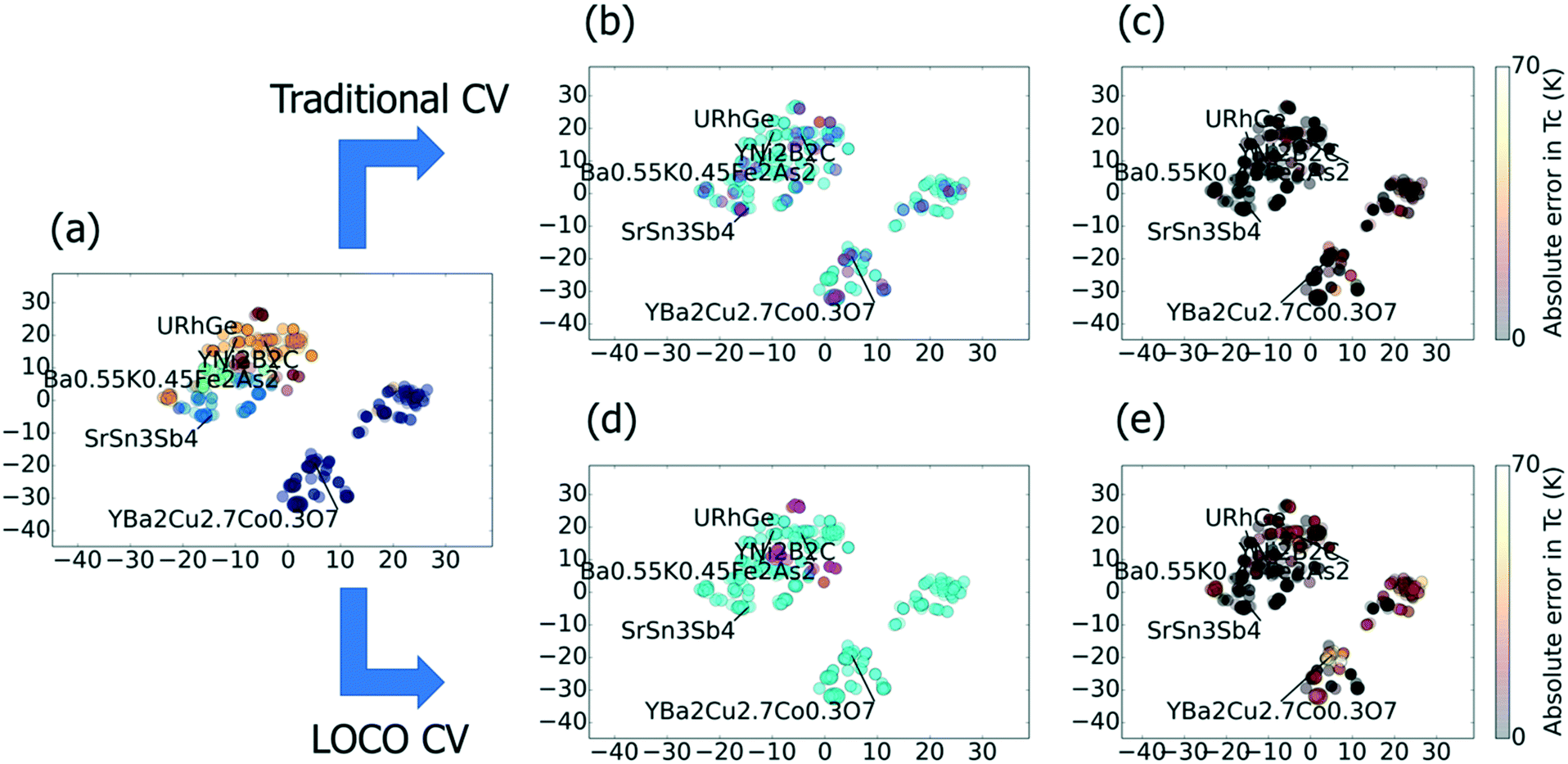 | ||
| Fig. 1 A two-dimensional t-SNE projection of the superconductor benchmark dataset, which visualizes local chemical similarity. Note: the x and y axes do not have precise physical meaning in a t-SNE plot. (a) Chemical distribution of a single 5-fold CV split for this dataset, where cyan points represent the training data (80% of examples) and the magenta points represent the test set (20% of examples). For each test material (magenta), a highly chemically similar (i.e., very near in chemical space) material is available as training input (cyan). (b) Absolute errors for traditional CV predictions of Tc for each material; these errors tend to be quite low due to the proximity of train and test points as shown in (a). (c) Results of k-means clustering on the superconductor dataset with k = 5 clusters. The clustering is performed on the full input feature space. (d) Example of one hold-out cluster in LOCO CV with k = 5. Note that, in LOCO CV, neighboring materials are grouped together and either “all in” (cyan) or “all out” (magenta; the labeled exemplar is YNi2B2C) of the training set. (e) Absolute errors for LOCO CV predictions of each material. The prediction errors are much greater than in random CV, because the ML model must generalize from the training clusters to a distinct test cluster. | ||
Fig. 1 gives two-dimensional t-distributed stochastic neighbor embedding (t-SNE)19 visualizations of the superconductor benchmark dataset, showing the effects of traditional and LOCO CV on predicting Tc. In this benchmark, a machine learning model is trained to predict the critical temperature as a function of chemical formula. The chemical formula is featurized using Magpie20 and other analytical features calculated based on the elemental composition. We observe in t-SNE that the superconductors cluster into well-known families, such as the cuprates and the iron arsenides. Such clustering is common in materials datasets, and provides motivation for LOCO CV. In Fig. 1a, which illustrates a typical 5-fold CV split, each magenta test point is very near (or virtually overlapping) in chemical space with a training point. The result, in Fig. 1b, is low Tc prediction errors across all families of superconductors. Fig. 1c and d show how LOCO CV partitions the YNi2B2C cluster into an isolated test set. The LOCO CV procedure, when repeated across all hold-out clusters, leads to much higher (and, we would argue, more realistic for materials discovery) errors in predicted Tc values when materials are part of the hold-out cluster, as indicated in Fig. 1e.
Leave-one-cluster-out cross-validation and extrapolation to new materials classes
The above considerations are well understood in other domains, such as ecology,21 where a variety of schemes exist to give a more realistic view of statistical model performance given known structure in the input space than is possible with traditional CV. However, the materials informatics community has devoted relatively little attention to the issue of extrapolating with models built on potentially highly-clustered training data. Stanev et al. recently applied ML to predict Tc for superconductors,22 wherein the authors discuss extrapolation from one class of superconductors to others (see, in particular, their Fig. 4). The authors conclude, “Models trained on a single group have no predictive power for materials from other groups”.22 The present work explores precisely this idea in more detail.To systematically explore the effects of non-uniform training data, we propose LOCO CV, a cluster-based (i.e., similarity-driven) approach to separating datasets into training and test splits. We outline LOCO CV as follows:
LOCO CV Algorithm.
• Perform standard normalization of input features.
• For n total CV runs:
○ Shuffle data to reduce sensitivity to k-means centroid initialization.
○ Run k-means clustering, with k from 2 to 10. These bounds correspond to the minimum possible value of k (i.e., 2) to k corresponding to the largest common choice of 10 folds in traditional CV.
○ For each of k clusters:
■ Leave selected cluster out; train on remainder of data (k-1 clusters).
■ Predict hold-out cluster.
• To summarize results across many values of k: compute median and standard deviation across k.
○ Alternative: use X-means23 or G-means24 clustering, or a silhouette factor threshold,25 to select a single nominal value of k.
To illustrate the sharp contrast between ML results with LOCO CV and conventional traditional CV, we contrast the prediction distributions obtained from these two CV procedures for yttrium barium copper oxide (YBCO) in Fig. 2. The traditional CV results seem to suggest that the underlying model is indeed capable of discovering new compounds like YBCO, with exceptional Tc values, in a single high-throughput screening step. Specifically, when YBCO is held out of the training set in traditional CV, the model still provides high predicted Tc values. One might then conclude that novel materials discovery would be enabled by running the model against a large database of candidate compounds and simply ranking them by predicted Tc. However, Fig. 2 suggests that traditional CV is utilizing other high-Tc cuprates to trivially estimate a reasonable (i.e., very high) Tc value for YBCO, while LOCO CV has no high-Tc cuprates to train on (indicated by the difference curve in Fig. 2 in the Tc > 80 K regime).
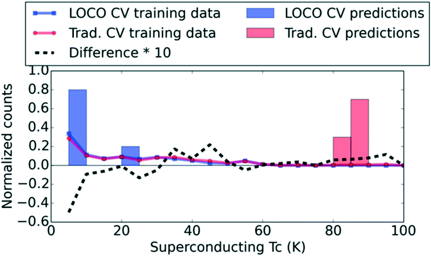 | ||
| Fig. 2 Prediction and training data distributions for YBCO within k = 10 LOCO CV and traditional 10-fold CV. The LOCO CV procedure prevents an ML model from predicting YBCO by trivially associating it with abundant training data on other cuprates; as a result, the LOCO CV Tc predictions are dramatically lower for YBCO. “Difference * 10” is the difference between the traditional and LOCO CV training data distributions, multiplied by 10 for clarity. | ||
The surprising LOCO prediction, which has no training data on cuprates due to its cluster-based train-test splitting, is that YBCO is likely to be a below-average superconductor. Nonetheless, Ling et al. show26 that ML with uncertainty quantification (UQ) can efficiently identify the highest-Tc superconductor in a database (i.e., breakthrough materials like YBCO) when used to iteratively guide experimentation in a sequential learning framework. Sequential learning (also known as active learning, on-the-fly learning, or adaptive design) is rapidly garnering interest as a driver for rational solid-state materials discovery,12,27–29 and has been applied successfully to organic molecules as well.30 For superconductors specifically, Ling et al. demonstrate that, starting from a very small, randomly-selected training set, an ML model that selects new “experiments” based on a criterion of maximum uncertainty in Tc will uncover the cuprates in consistently fewer experiments than an unguided search through the same list of superconductors.26 UQ enables ML to systematically uncover promising compounds, one experiment (or batch) at a time, even when those compounds may have e.g. a low predicted Tc in the initial screen. Thus, the use of UQ on top of ML models is crucial to evaluating candidates in new regions of design space. The ramifications of this observation deserve special emphasis: we suggest that ML models (and indeed, possibly other types of models in materials science) are more useful as guides for an iterative sequence of experiments, as opposed to single-shot screening tools that can reliably evaluate an entire search space once and short-list high-performing materials. Laboratory discoveries reported in Xue et al.12 and Ren et al.31 reinforce the efficacy of such an iterative, data-driven approach.
Benchmark results
Extrapolation and training data distribution are not trivial to disentangle in real-world problems, but we investigate LOCO CV performance on non-uniform training data by systematically varying “degree of clustering” on a synthetic problem. We define a simple analytical function of six variables as follows:f(x0,![[thin space (1/6-em)]](https://www.rsc.org/images/entities/char_2009.gif) x1,x2,x3,x4,x5) = x0·x1 + x2·x3 − x4·x5, x1,x2,x3,x4,x5) = x0·x1 + x2·x3 − x4·x5, |
We present ML results on this synthetic benchmark, as well as superconductor, steel fatigue strength, and thermoelectric benchmark datasets26 in Fig. 3. Using implementations in the scikit-learn32 python package, we compare three types of ML models. First, random forest33 (“RF”; 100 estimators, full-depth trees) is an ensemble method whose predictions are based on inputs from a large number of simple decision tree models (i.e., the trees comprising the “forest”). A set of decision trees, which individually are weak learners able to capture basic rules such as e.g. “large oxygen mole fraction → electrical insulator,” can—when trained on different subsets of data and subsequently ensembled—model (much) more complex relationships. Second, linear ridge regression34 (“ridge”; generalized CV was used to select from a set of possible regularization parameters α: 10−2, 10−1, 100, 101, and 102) involves extending the ordinary-least-squares (OLS) objective function of traditional linear regression with an L2 regularization term (whose strength is embodied in an adjustable parameter α) to penalize nonzero linear regression coefficients. Such regularization helps prevent overfitting, especially when collinear descriptors are present. Third, we include a naive nearest-neighbor (1NN) “lookup table” model, which generates predictions by simply returning the training value nearest in Euclidean distance to the requested prediction point; thus, it is by definition not capable of any extrapolation. In Fig. 3, the aforementioned three models are compared across traditional CV and LOCO CV; within LOCO CV, we use the scikit-learn32 implementation of k-means clustering. While the full CV curves contain valuable information, we also summarize Fig. 3 more compactly in Table 2.
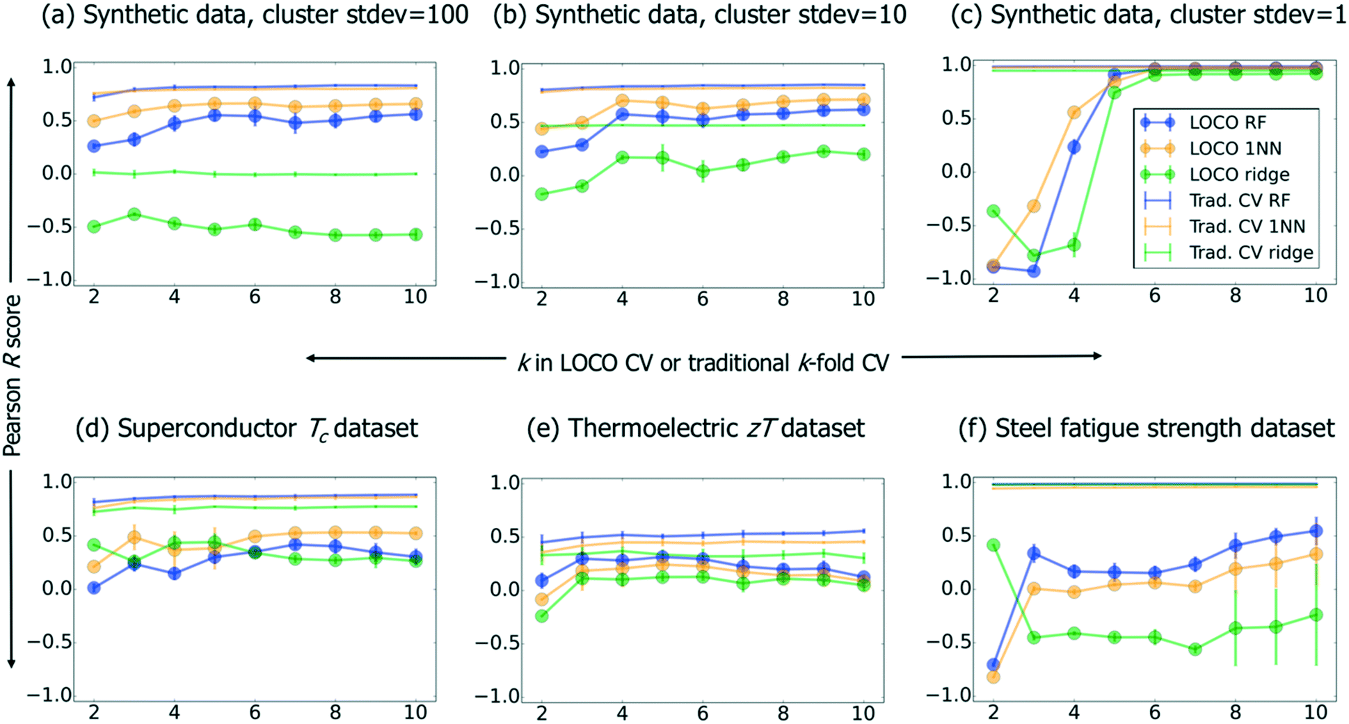 | ||
| Fig. 3 Pearson R vs. k in k-fold CV (traditional CV) or k-means clustering (LOCO CV) across our benchmark datasets and several ML methods. Error bars represent the sample standard deviation of R across 10 CV runs at each value of k. | ||
| Benchmark problem | LOCO RF median R (stdev) | LOCO 1NN median R (stdev) | LOCO ridge median R (stdev) | Traditional CV RF median R (stdev) | Traditional CV 1NN median R (stdev) | Traditional CV ridge median R (stdev) |
|---|---|---|---|---|---|---|
| Synthetic, stdev = 100 | 0.50 | 0.64 | −0.52 | 0.82 | 0.80 | 0.00 |
| (0.11) | (0.05) | (0.07) | (0.04) | (0.02) | (0.01) | |
| Synthetic, stdev = 10 | 0.57 | 0.68 | 0.17 | 0.84 | 0.82 | 0.47 |
| (0.14) | (0.10) | (0.14) | (0.02) | (0.01) | (0.00) | |
| Synthetic, stdev = 1 | 0.97 | 0.97 | 0.91 | 0.99 | 0.98 | 0.95 |
| (0.81) | (0.68) | (0.76) | (0.00) | (0.00) | (0.00) | |
| Superconductors log(Tc) | 0.30 | 0.50 | 0.30 | 0.87 | 0.85 | 0.76 |
| (0.13) | (0.11) | (0.08) | (0.02) | (0.03) | (0.02) | |
| Thermoelectrics log(zT) | 0.23 | 0.17 | 0.10 | 0.52 | 0.45 | 0.33 |
| (0.08) | (0.10) | (0.12) | (0.03) | (0.03) | (0.02) | |
| Steel fatigue strength | 0.24 | 0.05 | −0.41 | 0.99 | 0.96 | 0.98 |
| (0.37) | (0.33) | (0.29) | (0.00) | (0.00) | (0.00) |
We also wish to comment briefly on the motivation for our choice of the three ML approaches. 1NN is subjectively the simplest possible consistent estimator: in principle, given enough data, it can learn any function. On the other hand, a linear model is subjectively the simplest model that allows for the expression of bias (in the form of the model itself, which is linear), but linear ridge regression is not able to learn an arbitrary function. Finally, RFs are related to nearest-neighbor methods, but are much more powerful, and deliver close to state-of-the-art performance on chemistry problems.35
In Fig. 3a–c, we observe that stronger clustering in the synthetic data (i.e., decreasing cluster standard deviations) creates a stark feature in the R vs. k plot: a deep minimum in model performance when k corresponds to a “natural” number of clusters associated with the dataset (the synthetic dataset has three cluster centroids by construction). This effect leads to large standard deviations in LOCO CV performance across different values of k for clustered data (see Table 2), and suggests we should be skeptical of our ability to accurately assess model performance as clustering becomes more severe. Relatedly, we note that the 1NN model performs well in traditional CV for highly clustered data (synthetic dataset with stdev = 1, and also the steel fatigue strength benchmark). Finally, as random forest and 1NN are both neighborhood-based methods,36 we include a linear ridge regression to show that our conclusions also apply to non-neighborhood methods.
Table 2 shows that RF performs consistently best within traditional CV, which suggests that, when this algorithm has full information in the neighborhood around a test point, it can (as expected) make more accurate predictions than a nearest-neighbor model. Within LOCO CV, we see that while RF achieves the highest R values for the thermoelectric and steel fatigue benchmarks, it fails to outperform 1NN for superconductors and the synthetic data. This result, together with the remarkably strong performance of 1NN for highly clustered data, demonstrates that 1NN is an essential benchmark to contextualize performance of materials informatics models. In other words, ML can enable more efficient discovery of superconductors,26 even if a given ML model's ability to extrapolate directly to the cuprates is no better than that of a 1NN lookup table.
Our LOCO CV results reveal that one-shot extrapolation to entirely new materials classes, without formally taking degree-of-extrapolation into account (e.g., the notion of “distance control” presented by Janet, Chan and Kulik37), poses a significant challenge to ML. This observation, together with the work of Ling et al.,26 suggests that UQ-based sequential learning (i.e., the ability of ML to plan the iterative, systematic exploration of a search space) may be more important to data-driven materials discovery than making extremely accurate predictions of novel materials' properties. We thus frame the ideal application of ML in materials discovery as experiment prioritization, rather than materials property prediction, for which e.g. DFT is often used. We also note that the general difficulty for ML to extrapolate from one cluster (or physical regime) to another provides motivation for further work in transfer learning,38 and could help explain why multitask learning has exhibited some success on physical problems such as molecular property prediction.35
Conclusions
In this work, we identified some important limitations of traditional CV for evaluating ML model performance for materials discovery. We proposed new measures of model performance geared toward materials discovery, including LOCO CV and a naive 1NN “lookup table” baseline for materials property regression. Our results provide motivation for deeper investigations of the importance of UQ and sequential learning for materials discovery. LOCO CV also provides a path for selecting and tuning models for better performance across diverse groups of materials. Further work should formally link UQ to the observations herein, and explore how degree-of-extrapolation (as quantified by some distance function) influences model performance.Conflicts of interest
There are no conflicts to declare.Acknowledgements
This work was supported in part by NIST contract 60NANB15D077 and DOE contract DE-AC02-06CH11357. Certain commercial equipment, instruments, or materials are identified in this paper to foster understanding. Such identification does not imply recommendation or endorsement by the National Institute of Standards and Technology, nor does it imply that the materials or equipment identified are necessarily the best available for the purpose.Notes and references
- J. Hill, G. Mulholland, K. Persson, R. Seshadri, C. Wolverton and B. Meredig, MRS Bull., 2016, 41, 399–409 CrossRef.
- L. Ward and C. Wolverton, Curr. Opin. Solid State Mater. Sci., 2017, 21, 167–176 CrossRef.
- A. Agrawal, P. D. Deshpande, A. Cecen, G. P. Basavarsu, A. N. Choudhary and S. R. Kalidindi, Integr. Mater. Manuf. Innov., 2014, 3, 1–19 CrossRef.
- F. A. Faber, L. Hutchison, B. Huang, J. Gilmer, S. S. Schoenholz, G. E. Dahl, O. Vinyals, S. Kearnes, P. F. Riley and O. A. von Lilienfeld, J. Chem. Theory Comput., 2017, 13, 5255–5264 CrossRef PubMed.
- B. Meredig, A. Agrawal, S. Kirklin, J. E. Saal, J. W. Doak, A. Thompson, K. Zhang, A. Choudhary and C. Wolverton, Phys. Rev. B: Condens. Matter Mater. Phys., 2014, 89, 94104 CrossRef.
- F. Legrain, J. Carrete, A. van Roekeghem, S. Curtarolo and N. Mingo, Chem. Mater., 2017, 29, 6220–6227 CrossRef.
- J. Lee, A. Seko, K. Shitara, K. Nakayama and I. Tanaka, Phys. Rev. B, 2016, 93, 115104 CrossRef.
- S. Ubaru, A. Mikedlar, Y. Saad and J. R. Chelikowsky, Phys. Rev. B, 2017, 95, 214102 CrossRef.
- J. A. Gomberg, A. J. Medford and S. R. Kalidindi, Acta Mater., 2017, 133, 100–108 CrossRef.
- A. O. Oliynyk, E. Antono, T. D. Sparks, L. Ghadbeigi, M. W. Gaultois, B. Meredig and A. Mar, Chem. Mater., 2016, 28, 7324–7331 CrossRef.
- A. O. Oliynyk and A. Mar, Acc. Chem. Res., 2018, 51, 59–68 CrossRef PubMed.
- D. Xue, P. V. Balachandran, J. Hogden, J. Theiler, D. Xue and T. Lookman, Nat. Commun., 2016, 7, 11241 CrossRef PubMed.
- B. D. Conduit, N. G. Jones, H. J. Stone and G. J. Conduit, Mater. Des., 2017, 131, 358–365 CrossRef.
- J. H. Martin, B. D. Yahata, J. M. Hundley, J. A. Mayer, T. A. Schaedler and T. M. Pollock, Nature, 2017, 549, 365 CrossRef PubMed.
- Y. LeCun, http://yann. lecun. com/exdb/mnist/.
- K. Wu, N. Sukumar, N. A. Lanzillo, C. Wang, R. Ma, A. F. Baldwin, G. Sotzing, C. Breneman and others, J. Polym. Sci., Part B: Polym. Phys., 2016, 54, 2082–2091 CrossRef.
- J. Bennett, S. Lanning and others, in Proceedings of KDD cup and workshop, 2007, vol. 2007, p. 35 Search PubMed.
- Y. Zhou, D. Wilkinson, R. Schreiber and R. Pan, in International Conference on Algorithmic Applications in Management, 2008, pp. 337–348 Search PubMed.
- L. van der Maaten and G. Hinton, J. Mach. Learn. Res., 2008, 9, 2579–2605 Search PubMed.
- L. Ward, A. Agrawal, A. Choudhary and C. Wolverton, npj Comput. Mater., 2016, 2, 16028 CrossRef.
- D. R. Roberts, V. Bahn, S. Ciuti, M. S. Boyce, J. Elith, G. Guillera-Arroita, S. Hauenstein, J. J. Lahoz-Monfort, B. Schröder, W. Thuiller and others, Ecography, 2017, 40, 913–929 CrossRef.
- V. Stanev, C. Oses, A. G. Kusne, E. Rodriguez, J. Paglione, S. Curtarolo and I. Takeuchi, 2017, arXiv Prepr. arXiv1709.02727.
- D. Pelleg, A. W. Moore and others, in Icml, 2000, vol. 1, pp. 727–734 Search PubMed.
- G. Hamerly and C. Elkan, in Advances in neural information processing systems, 2004, pp. 281–288 Search PubMed.
- P. J. Rousseeuw, J. Comput. Appl. Math., 1987, 20, 53–65 CrossRef.
- J. Ling, M. Hutchinson, E. Antono, S. Paradiso and B. Meredig, Integr. Mater. Manuf. Innov., 2017, 6, 207–217 CrossRef.
- A. G. Kusne, T. Gao, A. Mehta, L. Ke, M. C. Nguyen, K.-M. Ho, V. Antropov, C.-Z. Wang, M. J. Kramer, C. Long and others, Sci. Rep., 2014, 4, 6367 CrossRef PubMed.
- T. Ueno, T. D. Rhone, Z. Hou, T. Mizoguchi and K. Tsuda, Mater. Discov., 2016, 4, 18–21 CrossRef.
- T. M. Dieb and K. Tsuda, in Nanoinformatics, Springer, 2018, pp. 65–74 Search PubMed.
- J. S. Smith, B. Nebgen, N. Lubbers, O. Isayev and A. E. Roitberg, J. Chem. Phys., 2018, 148(24), 241733 CrossRef PubMed.
- F. Ren, L. Ward, T. Williams, K. J. Laws, C. Wolverton, J. Hattrick-Simpers and A. Mehta, Sci. Adv., 2018, 4, eaaq1566 CrossRef PubMed.
- F. Pedregosa, G. Varoquaux, A. Gramfort, V. Michel, B. Thirion, O. Grisel, M. Blondel, P. Prettenhofer, R. Weiss, V. Dubourg, J. Vanderplas, A. Passos, D. Cournapeau, M. Brucher, M. Perrot and E. Duchesnay, J. Mach. Learn. Res., 2011, 12, 2825–2830 Search PubMed.
- A. Liaw, M. Wiener and others, R news, 2002, 2, 18–22 Search PubMed.
- A. E. Hoerl and R. W. Kennard, Technometrics, 1970, 12, 55–67 CrossRef.
- J. Ma, R. P. Sheridan, A. Liaw, G. E. Dahl and V. Svetnik, J. Chem. Inf. Model., 2015, 55, 263–274 CrossRef PubMed.
- Y. Lin and Y. Jeon, J. Am. Stat. Assoc., 2006, 101, 578–590 CrossRef.
- J. P. Janet, L. Chan and H. J. Kulik, J. Phys. Chem. Lett., 2018, 9, 1064–1071 CrossRef PubMed.
- M. L. Hutchinson, E. Antono, B. M. Gibbons, S. Paradiso, J. Ling and B. Meredig, 2017, arXiv Prepr. arXiv1711.05099.
| This journal is © The Royal Society of Chemistry 2018 |