
Statistical models are able to predict ionic liquid viscosity across a wide range of chemical functionalities and experimental conditions†
Wesley
Beckner
a,
Coco M.
Mao
a and
Jim
Pfaendtner
 *ab
*ab
aDepartment of Chemical Engineering, University of Washington, Seattle, Washington 98195, USA. E-mail: jpfaendt@uw.edu
bSenior Scientist, Pacific Northwest National Laboratory, Richland, Washington, USA
First published on 12th January 2018
Abstract
Herein we present a method of developing predictive models of viscosity for ionic liquids (ILs) using publicly available data in the ILThermo database and the open-source software toolkits PyChem, RDKit, and SciKit-Learn. The process consists of downloading ∼700 datapoints from ILThermo, generating ∼1200 physiochemical features with PyChem and RDKit, selecting 11 features with the least absolute shrinkage selection operator (LASSO) method, and using the selected features to train a multi-layer perceptron regressor—a class of feedforward artificial neural network (ANN). The interpretability of the LASSO model allows a physical interpretation of the model development framework while the flexibility and non-linearity of the hidden layer of the ANN optimizes performance. The method is tested on a range of temperatures, pressures, and viscosities to evaluate its efficacy in a general-purpose setting. The model was trained on 578 datapoints including a temperature range of 273.15–373.15 K, pressure range of 60–160 kPa, viscosity range of 0.0035–0.993 Pa s, and ILs of imidazolium, phosphonium, pyridinium, and pyrrolidinium classes to give 33 different salts altogether. The model had a validation set mean squared error of 4.7 × 10⁻⁴ ± 2.4 × 10⁻⁵ Pa s or relative absolute average deviation of 7.1 ± 1.3%.
Design, System, ApplicationThis work presents a method of developing viscosity models for ionic liquids (ILs). The process utilizes the python modules PyChem and SciKit-Learn and data from the ILThermo database provided by the National Institute of Standards and Technology (NIST). Beginning with a 1271 feature space, the optimization strategy includes parameterizing a least absolute shrinkage selection operator (LASSO) method, using bootstrap and LASSO to select and create confidence intervals for the top features, and training a neural network (NN). The final output is a NN with 11 features that is accurate for categorically different ILs across a broad range of temperature, pressure, and viscosity. We show that the method works with reasonable accuracy even when the NN has been trained on categorically ILs. This is especially true if, within the training data, at least either the cationic or anionic moiety has been encountered. Because the feature space does not include interaction parameters between the ions, the NN does not need to be retrained to evaluate new cation/anion pairs, a design constraint that has been typical of recent viscosity models. Future applications could include using the NN as a fitness test in evolutionary algorithms to search for ILs with desirable properties. |
Introduction
Recent years have seen a huge rise in the successful application of machine or statistical learning type approaches to the discovery and design of new materials. Efforts such as Materials Genome Initiative (MGI) have led to the creation of public data repositories like the Harvard Clean Energy Project,1 Materials Project,2 Open Quantum Materials Database (OQMD),3 and Automatic FLOW for Materials Discovery (AFLOW).4 In the area of solid crystalline materials, research pipelines based on high throughput calculations have enabled rapid population of massive databases. However, many important materials for a wide range of applications are liquids, including emerging solvent classes such as ionic liquids (ILs) or deep eutectic solvents.5 In contrast to crystalline materials, liquids present a host of challenges that prevent direct mimic of the successful MGI type approaches. For example, calculation of relevant properties with molecular simulations requires statistical sampling (e.g., molecular dynamics (MD) or Monte Carlo) compared with the energy minimization and structural calculations used in solid systems. Intrinsic properties of liquids show much stronger dependence on thermodynamic state variables. Finally, in a potential advantage compared to crystalline materials, public datasets of experimental measurements such as those available from NIST Webbook offer huge opportunities for training statistical learning models.Many of the current applications of linear and non-linear statistical learning methods in physical sciences are inspired by studies using quantitative structure–property relationships, QSPR; or quantitative structure–activity relationships, QSAR, which were widely used starting in the 1960s and beyond.6,7 The thousands of QSPR/QSAR models that have been developed in the previous half century have incited both praise and criticism of their reliability and limitations.8,9 In response to this and in the interest of promoting high-quality models, the Organization for Economic Co-operation and Development (OECD) developed five guiding principles; that a QSAR/QSPR model should have: 1) a defined endpoint, 2) an unambiguous algorithm, 3) a defined domain of applicability, 4) appropriate measures of goodness of fit, robustness and predictive-power, and 5) a mechanistic interpretation when possible.10 In the interest of objectives 4) and 5) some have stressed creating a small and focused set of descriptors for model development.11 Others have stressed resourcing the highest levels of domain area knowledge and statistical knowledge, via collaborations between experimental and computational scientists when necessary, to aid with these objectives.8 However, the continued exponential growth in available data, computing power, and open source software, further complicates the challenge by affecting the weight one would appropriate to any one of these principles. For instance, the modern ability to access extremely large experimental datasets and chemical search spaces introduces quite a different problem than that in the pioneering work of Hansch, Leo, and others,7 where relatively small datasets confined them to a limited feature space.
Taking into account these guidelines and the realities of dealing with ever-growing data sets,12 this paper describes our application of statistical machine learning models to the prediction of the viscosity of ionic liquid (IL) solvents. ILs have great potential for application in nanomaterials synthesis, bioremediation, and bio-catalysis/enzyme stabilization.5 They have also been identified as a potential supporting electrolyte material for redox flow batteries (RFBs).13–15 Especially in the case of RFBs, the solvent viscosity is critical to understand and control as it directly relates to the device's efficiency (via the total energy density). Within RFBs, there are two primary methods of increasing the energy density, and therefore efficiency, of a flow battery: 1) increasing the solubility of the active material or 2) reducing the viscosity of the electrolyte.16–18 Both of these methods are a consequence of having to actively pump the electrolyte across a membrane to facilitate charge transfer—one would desire that, that volume of fluid have either a high chemical potential energy or a low viscosity. Unfortunately these two characteristics, energy density and viscosity, have tended to be inversely correlated. It is for this reason that an accurate algorithm to determine viscosity based on the molecular constituents of an IL is extremely valuable. With these challenges in mind, we set out to use the public data available in the NIST ILThermo19 database for training and testing of different predictive models.
Apart from RFBs, in many applications the viscosity of the IL plays a huge economical factor; essentially whenever active transport of the IL is needed. Because of this, many predictive models of IL viscosity have been attempted. They have, however, been largely unsuccessful due to either not reproducing experimental values across categorically different ILs or requiring the use of IL-specific experimental data in predictions.20–30 Briefly, Matsuda et al. employed group contribution (GC) type descriptors with some accuracy. Their model, however, did not perform very well on a test dataset, reporting an R-squared value of 0.6226.30 Another GC approach was introduced by Gardas and Coutinho, where they fit the GC-type inputs to the Vogel–Tammann–Fulcher (VTF) equation. This is considered to be one of the most accurate, temperature dependent viscosity models to date but is limited to a narrowly defined set of ILs.25,28 Zhao et al., used GC-VTF methods to parameterize a UNIFAC-VISCO model. While they reported a low error rate for the regression on their training data, their model is meant to predict binary mixtures of ILs and so is not very useful in terms of exploring a structural search space.31 As a last look at the GC-type models, Padusyzński & Domańska did an extensive data scraping of the literature to produce a feed forward artificial neural network (FF-ANN) using GC-type inputs and Fatehi et al. applied an FF-ANN to GC-type inputs supplemented with electronegativity descriptors.25,32 Their models did very well across many IL types. They did not however, examine how their models might perform given an IL type from outside their training data, something we determine for our model in this work.
Other attempts at IL viscosity models have been made without the use of GC-type inputs, notably, hole theory models by Bandrés et al. and volumetric VTF models by Slattery et al., but have required the use of experimental data in some form or another.27,29 In this work, we introduce a method to accurately predict viscosity for categorically different ILs and broad ranges of temperature (T), pressure (P), and viscosity. Additionally, we explore the sensitivity of the approach to underlying molecular structure and include these results in the ESI.†
The remainder of this manuscript is organized as follows. The next section combines methodological details with the model development. Following this we apply linear and nonlinear statistical learning methods to understand key structural predictors of viscosity and provide robust statistical analysis on a large data set of experimentally measured IL viscosities. Finally, we discuss the applicability of the model across different IL types as well as the underlying features that explain the variance in the viscosity across our training data.
Methods and model development
Data collection and structure dependence
Many prior attempts to model IL viscosity21,22,31,33–35 required narrow definition of cation or anion classes. Therefore, we filtered our starting dataset to emphasize variance in structure in an attempt to understand the limits of a single statistical model. We began with 1405 experimental data points from the ILThermo database and screened for a T range of 273.15–373.15 K, P range of 60–160 kPa, and viscosity range of 0.0035–0.993 Pa s. The original dataset (including experimental references) before screening is available in the ESI† as viscosity_data.csv. Classes of structure included imidazolium, phosphonium, pyridinium, and pyrrolidinium based salts. After this initial screening, the final dataset contained 723 data points consisting of 33 unique salts; 22 anions and 16 cations. We then created a subset of 28 unique imidazolium salts containing 403 data points including a temperature range of 273.15–373.15 K, pressure range of 100–160 kPa, viscosity range of 0.004229–0.982 Pa s. We then applied the following protocol to this subset to evaluate how our general model might perform on salt-types not included in its training data, see Fig. 1. | ||
| Fig. 1 723 data points with temperature, pressure, and viscosity ranges of 273.15–373.15 K, 60–160 kPa, and 0.0035–0.993 Pa s, respectively. Inset: 453 data points with temperature, pressure, and viscosity ranges of 273.15–373.15 K, 100–160 kPa, and 0.004229–0.982 Pa s, respectively. The imidazolium base structure is illustrated in the whitespace. | ||
Feature generation
The open source python packages PyChem36,37 and RDKit38 were used to generate 633 physiochemical descriptors for each cation and anion in the starting dataset (1266 per IL). T and P, 1/T, T2, and ln(T) were included in the feature set to give a final data frame of dimensions 723 by 1271. All features were centered about zero and scaled to unit variance. After removing columns with zero variance the final data frame consisted of 723 data points with 771 descriptors. This data frame is included in the ESI† as viscosity_processed.csv.LASSO: model parameterization
The least absolute shrinkage and selection operator (LASSO)39 algorithm from the SciKit-learn40 machine learning toolkit was used to shrink the feature space. The primary hyper-parameter of the LASSO model (λ) was optimized in three separate schemes: 5-fold cross-validation (CV), shuffle-split, and bootstrap confidence test algorithms (see Fig. 2). Explained briefly, these algorithms break the data into 80/20 training/testing sets for 300 iterations. In the bootstrap scheme, the final training set is sampled from the training fraction with replacement, offering the possibility of the same data point being sampled multiple times. The shuffle-split schematic is identical to bootstrap apart from that the data is sampled without replacement; the original dataset is randomly shuffled and split between train and test. 5-fold CV was performed with slight modification. Keeping in line with the theme of the other methods, a random 80/20 split was made of the original dataset. 5-fold CV was then implemented in the standard way on the 80% fraction until the next iteration, in which another random 80/20 split was made. Each of these algorithms was implemented 300 times; trained and the mean squared error (MSE) evaluated on either 1) the testing portion of the dataset (bootstrap and shuffle-split) or 2) the aggregate from the five folds (5-fold CV).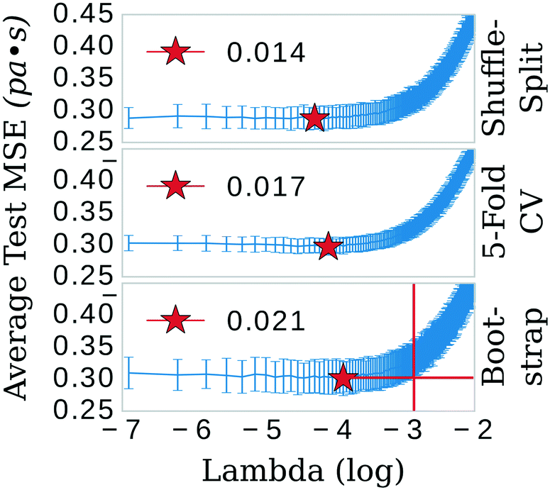 | ||
| Fig. 2 Shuffle-split, cross validation, and bootstrap algorithms were used to systematically search for the optimum λ value, the tuning parameter that determines the shrinkage penalty for LASSO. The red crosshairs in the bootstrap panel show that the most conservative (highest) value of λ, 0.021, is still within a standard deviation of the test MSE of a λ value as high as 0.054, i.e. a good selection for λ is highly contingent on the population of training data. | ||
LASSO: feature selection
The three confidence tests provided a starting point for feature shrinkage, however, the statistical variance in the test MSE indicated these optimum λ values were highly dependent on the randomly selected training data. Noting the bootstrap scheme in the bottom panel of Fig. 2, the average test MSE for a λ value of 0.021 was still within a standard deviation of the same test MSE for a λ value as high as 0.054 (or log![[thin space (1/6-em)]](https://www.rsc.org/images/entities/char_2009.gif) λ −2.9 in Fig. 2)—meaning, these two λ values share the same test MSE 68% of the time. While not certain, it is reasonable to posit that a λ value of 0.021 may be leaking noise into the model based on training data selections with incidental patterns in their feature vectors not related in any physical way to viscosity. To test for this, we selected 0.021 as the value for λ and trained the LASSO models on bootstrapped datasets for 1000 iterations to obtain confidence intervals for individual feature coefficients, see Fig. 3. A final, bootstrapped model was taken as the mean value of every non-zero return of the coefficients. This model was then used to predict viscosities for a validation set. Features were sorted by the absolute value of their mean and progressively removed from the model to determine at what point the test MSE no longer improved, see the insets of Fig. 3. Test MSE no longer improved after the top 11 most influential features were included in the models—regardless of whether all four categories of salt or only imidazolium-type salts constituted the training data. These top 11 features had p-values close to 0. After converging on the top 11 features, the LASSO models were trained at λ values ranging from 0 to 1 on their respective feature vectors. The expected approach to zero of the coefficients for each model are shown in Fig. 4.
λ −2.9 in Fig. 2)—meaning, these two λ values share the same test MSE 68% of the time. While not certain, it is reasonable to posit that a λ value of 0.021 may be leaking noise into the model based on training data selections with incidental patterns in their feature vectors not related in any physical way to viscosity. To test for this, we selected 0.021 as the value for λ and trained the LASSO models on bootstrapped datasets for 1000 iterations to obtain confidence intervals for individual feature coefficients, see Fig. 3. A final, bootstrapped model was taken as the mean value of every non-zero return of the coefficients. This model was then used to predict viscosities for a validation set. Features were sorted by the absolute value of their mean and progressively removed from the model to determine at what point the test MSE no longer improved, see the insets of Fig. 3. Test MSE no longer improved after the top 11 most influential features were included in the models—regardless of whether all four categories of salt or only imidazolium-type salts constituted the training data. These top 11 features had p-values close to 0. After converging on the top 11 features, the LASSO models were trained at λ values ranging from 0 to 1 on their respective feature vectors. The expected approach to zero of the coefficients for each model are shown in Fig. 4.
 | ||
| Fig. 3 Confidence intervals for the most influential features in the respective LASSO models. Insets show that the mean squared error does not improve past the 11 (red, vertical bar) most influential features. Models were trained 1000 times on bootstrapped datasets. X-axis displays the absolute values of the coefficients (values below the red, horizontal line are negative). Y-axis is sorted in ascending order (top to bottom) by the mean value of the coefficient. Green line indicates the median value, red box indicates the mean value, blue box indicates the 2nd and 3rd quantiles, and small, red bars indicate the range. The p-values for all coefficients are very close to zero, with the highest being 1 × 10−66. | ||
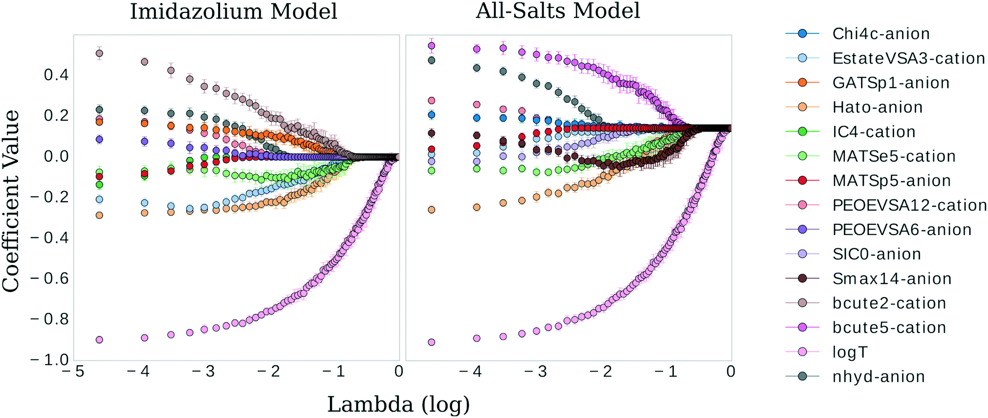 | ||
| Fig. 4 Coefficient values versus logλ for the most influential features in the imidazolium and general model, respectively. | ||
Neural network
The respective selected feature sets were used to train neural networks. The random search algorithm, RandomizedSearchCV was used to parameterize the multilayer perceptron (MLP) Regressor algorithm (a type of FF-ANN), both from SciKit-Learn. In the random search algorithm, ten settings were tested among the following distributions for the specified parameter. For activation: identity, logistic, tanh, and relu; for solver: limited memory Broyden–Fletcher–Goldfarb–Shanno algorithm (lbfgs), stochastic gradient descent (sgd), and adam; for learning rate: constant, invscaling, and adaptive; and a uniform distribution from zero to one was sampled for the regularization parameter, α. The listed parameter values were sampled without replacement while the uniform distribution for α was sampled with replacement. The final, selected settings for the specified parameter were the following. For activation: tanh, specifying a hyperbolic tan function for the activation function of the hidden layer; for solver: lbfgs, specifying a quasi-Newton method of solving for the weight optimization (a fast and accurate solver for smaller datasets, note that this stochastic solver recalculates its learning rate, α, at every step and nullifies any user-specified starting α); and max_iter: 1e8, the maximum number of iterations.The remaining parameters were left at their default values: batch_size: auto; early_stopping: false; hidden_layer_sizes: 100; random_state: none; validation_fraction: 0.1; warm_start: false. A full description of these parameters are available in the SciKit-Learn documentation.40
Final evaluation
For both the LASSO and the final ANN, bootstrapping was performed to estimate the variance in the predictions of a validation set. In the typical case, bootstrapping is a method of “internal validation” where subsets of the data are sampled with replacement and the resulting model is evaluated on the data excluded from the sample. The process is repeated to obtain error estimates for the entire dataset.41,42 We adapted this typical use case with “external validation” i.e. a portion of our dataset was reserved for validation, was never included in the model training, and the resulting models were used to obtain error estimates for this validation set. The process was as follows. For the ANN model, an 80–10–10% split of the entire dataset was used for train-test-validation. Bootstrapping was performed on the 80–10% sets and validated on the same 10% validation set for 300 iterations (i.e. the validation set data never entered the training data). The same procedure was performed on the imidazolium salt-types only—this time using the other salt-types as the validation set—to investigate how the general model might perform when exposed to salt-types not included in its training data. The procedure was identical for the LASSO model with the exception that a 90–10% split was made between training and validation since a test set is not required to determine the LASSO coefficients.Results and discussion
LASSO: feature selection
There have been prior approaches to develop models that predict viscosities for ILs. Few of them, however, have been successful across categorically different ILs.20–24 We investigated the dependency of our approach on structure by applying our procedure on only imidazolium-type salts, investigating the difference in selected features from the general model, and evaluating the ANN performance on the remaining three categories of salts. These selections of the data had a similar distribution of viscosity, T, and P to isolate the dependency of the model on core IL structure, see Fig. 1.The LASSO was used to shrink the physiochemical feature space. The selected features were similar between the imidazolium and general model, see Fig. 3. Both models consistently under-predicted viscosity values whose true values were above 0.2 Pa s and over-predicted the values of those below. The general LASSO model on average had a validation set error of 0.0108 ± 0.0008 Pa s while the imidazolium LASSO model had a higher validation set error of 0.025 ± 0.003 Pa s when evaluated on non-imidazolium salts and—as expected—a lower validation set error when evaluated on imidazolium salts, 0.0079 ± 0.0006 Pa s.
Description of the selected features
In the following we briefly explain the features that were selected by the imidazolium or general model, see also Table 1.| Descriptor | Type | Description |
|---|---|---|
| bcute5 | Autocorrelation | Burden autocorrelation of Sanderson electronegativity with topological interval 5 |
| bcute2 | Autocorrelation | Burden autocorrelation of Sanderson electronegativity with topological interval 2 |
| MATSp5 | Autocorrelation | Moran autocorrelation of polarizability with topological interval 5 |
| MATSe5 | Autocorrelation | Moran autocorrelation of Sanderson electronegativity with topological interval 5 |
| GATSp1 | Autocorrelation | Geary autocorrelation of polarizability with topological interval 1 |
| PEOEVSA12 | MOE | Sum of atomic van der Waals surface area contributions to partial charges within 0.25–0.3 |
| PEOEVSA6 | MOE | Sum of atomic van der Waals surface area contributions to partial charges within −0.05–0 |
| EstateVSA3 | MOE | Sum of atomic van der Waals surface area contributions to electropological states within 0.717–1.165 |
| SIC0 | Basak | Complementary information content with 0th order neighborhood of vertices in a hydrogen-filled graph |
| IC4 | Basak | Structural information content with 4th order neighborhood of vertices in a hydrogen-filled graph |
| Smax14 | Electropological | Maximum electrotopological state of sp hybridized carbon |
| Chi4c | Connectivity | Fourth order cluster index |
| Hato | Topological | Topological index of molecular branching |
The features are described extensively in the (ESI†) and additional information can be found in the corresponding references.
In the following acronyms the small letters signify the type of weighting used in the autocorrelation: atomic masses (m), van der Waals volumes (v), Sanderson electronegativities (e), atomic electronegativities (ae), and polarizabilities (p). The number represents the topological distance between atoms, i.e., the lag associated with the atomic property evaluated at those atomic points. Our models selected two Moran autocorrelations:44 MATSe5-cation and MATSp5-anion; two Burden autocorrelations:45 BCUTae5-cation and BCUTae2-cation; and one Geary autocorrelation:46 GATSp1-anion.
Inspecting the coefficients in Fig. 3, a negative Moran autocorrelation of the Sanderson electronegativities and polaraizabilities of the 5th topographical interval coincides with a decrease in viscosity in both models. In the imidazolium model, a positive Geary autocorrelation of polarizability on the 1st topographical interval coincides with an increase in viscosity. Burden autocorrelations of atomic electronegativies of the 2nd (imidazolium) and 5th (all salts) topographical interval coincides with an increase in viscosity in both models. Also of note, even with the large variance (the greatest in all the selected features by the model) in the Burden coefficients, the associated p-value is extremely low (1 × 10−66), indicating a high probability that this is a descriptive feature for viscosity.
Comparison between models
Of the five cation features selected by the imidazolium model, only MATSe5, E-state-VSA3, and PEOE-VSA12 were included in the general model. It is worth nothing, however, that the similar variance and mean value of the Burden features (BCUTEae5 and BCUTae2) for the cation imply a covariant relationship between these two variations of autocorrelating atomic electronegativity. A similar number of the anion-specific features are shared by both models: nhyd, MATSp5, and Hato. Indeed, the anionic features nhyd and Hato are extremely influential in both models (the absolute value of their coefficients are large), second only to log(T). For the cation-specific features: the imidazolium model included BCUTae2, and IC4 while the general model included BCUTae5. For the anion-specific features: the imidazolium model included GATSp1 and PEOE-VSA6 while the general model included Chi4c, SIC0, and Smax14. Interestingly, despite the structural difference between the two models being that of the cationic moiety, the largest difference in the feature vectors pertains to the anion (four shared features with a fifth that is likely to be covariant for the cation compared to three shared features for the anion). At first this would appear unlikely, even more so when considering the cation/anion differences between the models—22 anions and 16 cations for the general model and 21 anions and 10 cations for the imidazolium model. That is to say, even though the imidazolium model is only missing a single anion compared to the general model, it appears to select quite a different set of anion-specific features. However, considering the large coefficient values for the Hato and nhyd descriptors, the overall effect of the anionic moiety on viscosity is very similar for both models, as these two features have an overwhelming influence compared to the other anionic features that are present.In addition to performing 1000 bootstrap iterations of training LASSO at the optimum λ value, we also evaluated the coefficient values of those top selected features at λ values ranging from 0.01 to 1 to track their approach to 0. One might expect the feature coefficients to fall to zero in the order of their absolute value ranking at λ 0.021. However, since two features working in tandem might better approximate the descriptive quality of one, this may very well not be the case.
There are clear parallels in both models. The features approach zero in three separate clusters. log(T) formed the first cluster in solitude, holding its coefficient value ahead of the other features at higher values of λ. The models begin to differ in the next two clusters. The inverse-ranked approach to zero of the second cluster is as follows; beginning with the imidazolium model: BCUTe2-cation, Hato-anion, MATSe5-cation, Estate-VSA3-cation, GATSp1-anion; for the general model: Smax14-anion, BCUTe5-cation, MATSe5-cation, and Hato-anion. The inverse-ranked approach to zero of the third cluster is as follows; beginning with the imidazolium model: nhyd-anion, PEOE-VSA6-anion, PEOE-VSA12-cation, MATSp5-anion, and IC4-cation; for the general model: SIC0-anion, Chi4c-anion, Estate-VSA3-cation, nhyd-anion, MATSp5-anion, and PEOE-VSA12-cation.
There are a few interesting observations worth noting. First, although the Burden descriptors had the highest variance, p-values, and very low coefficients at λ 0.021, they both were included in the second cluster. This indicates that although descriptive, the response of this variable to selections of the underlying training data varies greatly. Second, the Moran autocorrelations MATSe5 and MATSp5 appear covariant: they both approach zero but as MATSp5 becomes zero, MATSe5 begins to increase and doesn't hit zero until the second cluster. Lastly, a qualitative comparison can be made between log(T) and the molecular coefficients. log(T) approaches zero on a very smooth curve, regardless of the behavior of the other features. In comparison, the physiochemical features in the model approach zero tortuously, acting in response to one another to some degree in all cases.
Neural network
The general ANN model was highly accurate on its validation set, with validation set MSE of 4.7 × 10⁻⁴ ± 2.4 × 10⁻⁵ Pa s, see Fig. 5. Recently, Zhao, et al.23 published a UNIFAC-VISO model of IL viscosity for the same class of structures but a narrower range of temperature (293.15–363.15 K) and a single pressure (0.1 mPa). Their approach resulted in a relative absolute average deviations (RAAD) of 3.92% on a test set with the caveat that their test set contained structurally identical ILs as that of the training data, only differing by the mole fractions of the binary IL mixtures. Converting our validation MSE to RAAD,56 we have a comparative performance in our final general ANN model of 7.1 ± 1.3 %. Table S1 in the ESI† breaks this RAAD down by structure and T. Perhaps more relevant, Padusyzński & Domańska reported a testing set RAAD (reported as AARD in their publication) of 14.7% for their GC FF-ANN model for nine classes of pure ILs with a broad range of temperature and pressure (253–573 K and 0.1–350 mPa, respectively). A comparison of these results and others are presented in Table 2.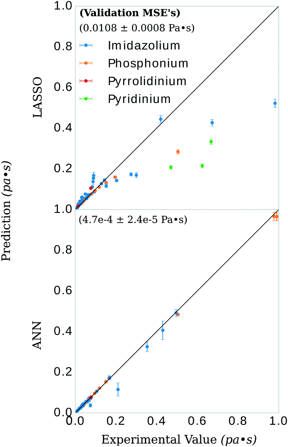 | ||
| Fig. 5 Viscosity prediction versus experimental value for the models. The bootstrap was performed on 90% of the available data. The remaining 10% of the data is shown in the figure, along with the prediction and error estimates from the bootstrap models. These error estimates are produced from the variance in the aggregate predictions of all the bootstrapped models. Some of the predictions have a relatively high variance compared to others. There are two possible explanations for this. For one, higher viscosities will inherently have a larger variance simply due to scaling (the same percent variance will appear larger for higher raw values of viscosity, note the two phosphonium predictions in the top right corner, bottom panel). Second, some of the anion-types occur in salt pairs less often than others. Subsequently, whether or not that anion appeared in the subsampled training set will influence the prediction on the validation datum. The three imidazolium-type salts with the highest variance contained either tetrafluoroborate or dimethylphosphate as their anions. The inset numbers indicate the value and standard deviation of the error for both models. The ANN models had, on average, mean squared errors of 4.7 × 10⁻⁴ Pa s for all data points in the validation set and a standard deviation of 2.4 × 10⁻⁵ Pa s for viscosity values ranging from 0.006 to 0.99 Pa s—an error that translates into a relative absolute average deviation (RAAD) of 7.1 ± 1.3%. Top: LASSO model; bottom: ANN model. | ||
| Structurally predictive | Pure or mixed IL | Model | Parameters | Data points | Test set error | Disadvantage | Reference |
|---|---|---|---|---|---|---|---|
| a 16 parameters per IL pair (32 parameters for binary mixtures). b At least 200 data points collected per IL, eight ILs were included in final regression. c Three parameters for VTF model, two of which were determined from 24 GC parameters. d The test datasets were provided by Padusyzński & Domańska, not the original authors. e The authors reported an R2 of 0.6226 on a test data set. | |||||||
| Yes | Pure | Physiochemical FF-ANN | 11 | 723 | 7.1 % | Higher test set error than comparable FF-ANN | Our model |
| Yes | Pure | Physiochemical FF-ANN | 13 | 736 | 1.3 % | Not tested on categorically different ILs from training data | Fatehi et al., 2017 (ref. 32) |
| Yes | Pure | GC FF-ANN | 242 | 13470 |
14.7 % | Not tested on categorically different ILs from training data | Padusyzński & Domańska, 2014 (ref. 25) |
| No | Pure/mixed | UNIFAC-VISCO GC VTF | 16/32a | 52 | 3.92 % | Requires pure IL experimental viscosity data | Zhao et al., 2016 (ref. 23) |
| No | Pure/mixed | QSPR | N/A | 5046 | N/A | QSPRs proposed without model | Yu et al., 2012 (ref. 26) |
| No | Pure | Hole theory | 7 | 8b | N/A | Requires experimental surface tension data | Bandrés et al., 2011 (ref. 27) |
| Yes | Pure | GC VTF | 3/24c | 482 | 13–21%d | Applicable to limited set of ILs | Gardas & Coutinho, 2009 (ref. 28) |
| Semi | Pure | Volumetric VTF | 3 | 23 | 9% | Some coefficients are anion-specific, others require QM calculations | Slattery et al., 2007 (ref. 29) |
| Yes | Pure | GC | 8 | 300 | N/Ae | Poor prediction for test dataset | Matsuda et al., 2007 (ref. 30) |
As discussed throughout this document, we are interested in how the general model would perform when predicting viscosity for salt-types not included in its training data (i.e. imidazolium, phosphonium, pyridinium, and pyrrolidinium). As a proxy for this, we applied the same protocol to the imidazolium salt-types only and—after observing the changes in selected descriptors in the previous section—evaluated the model on the other three salt-types. This model had a validation set MSE of 0.006 ± 0.001 Pa s when evaluated on imidazolium ILs and a validation set MSE of 0.08 ± 0.01 Pa s when evaluated on the non-imidazolium ILs: phosphonium, pyridinium, and pyrrolidnium. This leads us to emphasize caution when applying the general model to salts that are very structurally different than those used in the training data. The comparison of prediction vs. experimental viscosity is presented in the ESI,† Fig. S1. To our knowledge, other statistical models in the literature have not performed a similar such evaluation. We stress, however, that considering salt-types not in the training data is paramount in the construction of a predictive model for the purposes of designing as-of-yet undiscovered ILs.
Conclusions
We have demonstrated a method of generating accurate models for viscosity using publicly available data from ILThermo and open source software PyChem, RDKit and SciKit-Learn. We present a model that is highly predictive of viscosity across categorically different IL's: imidazolium, phosphonium, pyridinium, and pyrrolidinium based salts. We also evaluated the methodology by which we produced those models; applying the same steps but to a structural separate subset of our data—the imidazolium salts—and tested the model on salt-types it had not seen in its training set, the phosphonium, pyridinium, and pyrrolidinium salts. We found that with structurally different training data, the imidazolium model was able to encapsulate viscosity trends for the other salt-types.The methodology of using LASSO to pre-select features to then use in a neural network allowed us to benefit from the high interpretability of the LASSO method but also the high flexibility of the neural net. That is, we could evaluate the physical/chemical significance of the features that were selected while also arriving at a highly accurate model with the final neural network. It also allowed more rapid parameterization of the neural net and to avoid overfitting to our training data; i.e. keeping the feature size to training data ratio as low as possible.
In future work, the full value of the models should be actualized by combining them with structural search algorithms to high-throughput screen for low viscosity ILs. One of the most promising search algorithms recently introduced have been genetic algorithms, which allow for flexible fitness tests and a tree-like search structure. The fitness tests can prioritize certain model features, such as those ranked highest by the LASSO coefficient versus logλ evaluations, searching a semi-infinite structural space.
Conflicts of interest
There are no conflicts to declare.Acknowledgements
This project was funded under the Data Intensive Research Enabling Clean Technology (DIRECT) NSF National Research Traineeship (DGE-1633216).Notes and references
- J. Hachmann, R. Olivares-Amaya, S. Atahan-Evrenk, C. Amador-Bedolla, R. S. Sánchez-Carrera and A. Gold-Parker, et al., The harvard clean energy project: Large-scale computational screening and design of organic photovoltaics on the world community grid, J. Phys. Chem. Lett., 2011, 2(17), 2241–2251 CrossRef CAS.
- A. Jain, S. P. Ong, G. Hautier, W. Chen, W. D. Richards and S. Dacek, et al., Commentary: The materials project: A materials genome approach to accelerating materials innovation, APL Mater., 2013, 1(1), 0–11 CrossRef.
- J. E. Saal, S. Kirklin, M. Aykol, B. Meredig and C. Wolverton, Materials design and discovery with high-throughput density functional theory: The open quantum materials database (OQMD), JOM, 2013, 65(11), 1501–1509 CrossRef CAS.
- S. Curtarolo, W. Setyawan, S. Wang, J. Xue, K. Yang and R. H. Taylor, et al., AFLOWLIB.ORG: A distributed materials properties repository from high-throughput ab initio calculations, Comput. Mater. Sci., 2012, 58, 227–235 CrossRef CAS.
- A. Abo-Hamad, M. Hayyan, M. A. AlSaadi and M. A. Hashim, Potential applications of deep eutectic solvents in nanotechnology, Chem. Eng. J., 2015, 273, 551–567 CrossRef CAS.
- C. Nantasenamat, C. Isarankura-Na-Ayudhya, T. Naenna and V. Prachayasittikul, A practical overview of quantitative structure-activity relationship, EXCLI J., 2009, 8, 74–88 Search PubMed.
- A. Leo, C. Hansch and C. Church, Comparison of parameters currently used in the study of structure-activity relationships, J. Med. Chem., 1969, 12(5), 766–771 CrossRef CAS PubMed.
- A. Cherkasov, E. N. Muratov, D. Fourches, A. Varnek, I. I. Baskin and M. Cronin, et al., QSAR modeling: where have you been? Where are you going to?, J. Med. Chem., 2014, 57(12), 4977–5010 CrossRef CAS PubMed.
- A. Tropsha, Best practices for QSAR model development, validation, and exploitation, Mol. Inf., 2010, 29(6–7), 476–488 CrossRef CAS PubMed.
- J. C. Dearden, M. T. D. Cronin and K. L. E. Kaiser, How not to develop a quantitative structure–activity or structure–property relationship (QSAR/QSPR), SAR QSAR Environ. Res., 2009, 20(3–4), 241–266 CrossRef CAS PubMed.
- P. A. Labute, widely applicable set of descriptors, J. Mol. Graphics Modell., 2000, 18(4–5), 464–477 CrossRef CAS PubMed.
- D. A. C. Beck, J. M. Carothers, V. R. Subramanian and J. Pfaendtner, Data science: Accelerating innovation and discovery in chemical engineering, AIChE J., 2016, 62(5), 1402–1416 CrossRef CAS.
- M. A. Miller, J. S. Wainright and R. F. Savinell, Communication—Iron ionic liquid electrolytes for redox flow battery applications, J. Electrochem. Soc., 2016, 163(3), A578–A579 CrossRef CAS.
- M. H. Chakrabarti, F. S. Mjalli, I. M. AlNashef, M. A. Hashim, M. A. Hussain and L. Bahadori, et al. Prospects of applying ionic liquids and deep eutectic solvents for renewable energy storage by means of redox flow batteries, Renewable Sustainable Energy Rev., 2014, 30, 254–270 CrossRef CAS.
- D. Lloyd, Redox reactions in deep eutectic solvents: characterisation and application, School of Chemical Technology, 2013 Search PubMed.
- Q. Xu and T. S. Zhao, Fundamental models for flow batteries, Prog. Energy Combust. Sci., 2015, 49, 40–58 CrossRef.
- W. Wang, Q. Luo, B. Li, X. Wei, L. Li and Z. Yang, Recent progress in redox flow battery research and development, Adv. Funct. Mater., 2013, 23(8), 970–986 CrossRef CAS.
- A. Z. Weber, M. M. Mench, J. P. Meyers, P. N. Ross, J. T. Gostick and Q. Liu, Redox flow batteries: A review, J. Appl. Electrochem., 2011, 41(10), 1137–1164 CrossRef CAS.
- Q. Dong, C. D. Muzny, A. Kazakov, V. Diky, J. W. Magee and J. A. Widegren, et al. ILThermo: A free-access web database for thermodynamic properties of ionic liquids, J. Chem. Eng. Data, 2007, 52(4), 1151–1159 CrossRef CAS.
- M. H. Ghatee, M. Zare, A. R. Zolghadr and F. Moosavi, Temperature dependence of viscosity and relation with the surface tension of ionic liquids, Fluid Phase Equilib., 2010, 291(2), 188–194 CrossRef CAS.
- R. L. Gardas and J. A. P. Coutinho, A group contribution method for viscosity estimation of ionic liquids, Fluid Phase Equilib., 2008, 266(1–2), 195–201 CrossRef CAS.
- A. Fernández, J. García, J. S. Torrecilla, M. Oliet and F. Rodríguez, Volumetric, transport and surface properties of [bmim][MeSO4] and [emim][EtSO4] ionic liquids as a function of temperature, J. Chem. Eng. Data, 2008, 53(7), 1518–1522 CrossRef.
- N. Zhao, R. Oozeerally, V. Degirmenci, Z. Wagner, M. Bendová and J. Jacquemin, New method based on the UNIFAC–VISCO model for the estimation of ionic liquids viscosity using the experimental data recommended by mathematical gnostics, J. Chem. Eng. Data, 2016, 61(11), 3908–3921 CrossRef CAS.
- I. Billard, G. Marcou, A. Ouadi and A. Varnek, In silico design of new ionic liquids based on quantitative structure-property relationship models of ionic liquid viscosity, J. Phys. Chem. B, 2011, 115(1), 93–98 CrossRef CAS PubMed.
- K. Paduszyński and U. Domańska, Viscosity of ionic liquids: An extensive database and a new group contribution model based on a feed-forward artificial neural network, J. Chem. Inf. Model., 2014, 54(5), 1311–1324 CrossRef PubMed.
- G. Yu, D. Zhao, L. Wen, S. Yang and X. Chen, Viscosity of ionic liquids: Database, observation, and quantitative structure-property relationship analysis, AIChE J., 2012, 58(9), 2885–2899 CrossRef CAS.
- I. Bandrés, R. Alcalde, C. Lafuente, M. Atilhan and S. Aparicio, On the viscosity of pyridinium based ionic liquids: An experimental and computational study, J. Phys. Chem. B, 2011, 115(43), 12499–12513 CrossRef PubMed.
- R. L. Gardas and J. A. P. Coutinho, Group contribution methods for the prediction of thermophysical and transport properties of ionic liquids, AIChE J., 2009, 55(5), 1274–1290 CrossRef CAS.
- J. M. Slattery, C. Daguenet, P. J. Dyson, T. J. S. Schubert and I. Krossing, How to predict the physical properties of ionic liquids: A volume-based approach, Angew. Chem., Int. Ed., 2007, 46(28), 5384–5388 CrossRef CAS PubMed.
- H. Matsuda, H. Yamamoto, K. Kurihara and K. Tochigi, Computer-aided reverse design for ionic liquids by QSPR using descriptors of group contribution type for ionic conductivities and viscosities, Fluid Phase Equilib., 2007, 261(1–2), 434–443 CrossRef CAS.
- N. Zhao and J. Jacquemin, New method based on the UNIFAC-VISCO model for the estimation of dynamic viscosity of (ionic liquid + molecular solvent) binary mixtures, Fluid Phase Equilib., 2017, 449, 41–51 CrossRef CAS.
- M.-R. Fatehi, S. Raeissi and D. Mowla, Estimation of viscosities of pure ionic liquids using an artificial neural network based on only structural characteristics, J. Mol. Liq., 2017, 227, 309–317 CrossRef CAS.
- J. M. Crosthwaite, M. J. Muldoon, J. K. Dixon, J. L. Anderson and J. F. Brennecke, Phase transition and decomposition temperatures, heat capacities and viscosities of pyridinium ionic liquids, J. Chem. Thermodyn., 2005, 37(6), 559–568 CrossRef CAS.
- R. Bini, M. Malvaldi, W. R. Pitner and C. Chiappe, QSPR correlation for conductivities and viscosities of low-temperature melting ionic liquids, J. Phys. Org. Chem., 2008, 21(7–8), 622–629 CrossRef CAS.
- M. Barycki, A. Sosnowska, A. Gajewicz, M. Bobrowski, D. Wileńska and P. Skurski, et al., Temperature-dependent structure-property modeling of viscosity for ionic liquids, Fluid Phase Equilib., 2016, 427, 9–17 CrossRef CAS.
- PyChem.
- D. S. Cao, Q. S. Xu, Q. N. Hu and Y. Z. Liang, ChemoPy: Freely available python package for computational biology and chemoinformatics, Bioinformatics, 2013, 29(8), 1092–1094 CrossRef CAS PubMed.
- G. Landrum, RDKit: Open-source cheminformatics [Internet], [cited 2017 Nov 9], Available from: http://www.rdkit.org Search PubMed.
- R. Tibshirani, Regression shrinkage and selection via the LASSO, J. R. Stat. Soc. Series B Stat. Methodol., 1996, 58(1), 267–288 Search PubMed.
- F. Pedregosa, G. Varoquaux, A. Gramfort, V. Michel, B. Thirion and O. Grisel, et al., Scikit-learn: Machine learning in python, J. Mach. Learn. Res., 2012, 12, 2825–2830 Search PubMed.
- R. Veerasamy, H. Rajak, A. Jain, S. Sivadasan, C. P. Varghese and R. K. Agrawal, Validation of QSAR Models - Strategies and Importance, Int. J. Drug Des. Discovery, 2011, 2(3), 511–519 CAS.
- D. L. J. Alexander, A. Tropsha and D. A. Winkler, Beware of R2: Simple, Unambiguous Assessment of the Prediction Accuracy of QSAR and QSPR Models, J. Chem. Inf. Model., 2015, 55(7), 1316–1322 CrossRef CAS PubMed.
- P. Legendre, Spatial autocorrelation: Trouble or new paradigm?, Ecology, 1993, 74(6), 1659–1673 CrossRef.
- J. K. Ord and A. Getis, Local spatial autocorrelation statistics: Distributional issues and an application, Geogr. Anal., 1995, 27(4), 286–306 CrossRef.
- R. Todeschini and V. Consonni, Methods and Principles in Medicinal Chemistry, Handbook of Molecular Descriptors, Wiley-VCH Verlag GmbH, Weinheim, Germany, 2000, vol. 4, pp. 3–527 Search PubMed.
- R. C. Geary, The contiguity ratio and statistical mapping, Inc Stat, 1954, 5(3), 115 Search PubMed.
- L. Hall and L. Kier, The E-state as the basis for molecular structure space definition and structure similarity, J. Chem. Inf. Comput. Sci., 2000, 40(3), 784–791 CrossRef CAS PubMed.
- D. Butina, Performance of Kier-Hall E-state descriptors in quantitative structure activity relationship (QSAR) studies of multifunctional molecules, Molecules, 2004, 9(12), 1004–1009 CrossRef CAS PubMed.
- L. H. Hall and L. B. Kier, Electrotopological state indices for atom types: A novel combination of electronic, topological, and valence state information, J. Chem. Inf. Model., 1995, 35(6), 1039–1045 CrossRef CAS.
- B. Mohney, L. Kier and L. H. Hall, The electrotopological state: An atom index for QSAR, Quant. Struct.-Act. Relat., 1991, 10, 43–51 CrossRef.
- J. Gasteiger and M. Marsili, Iterative partial equalization of orbital electronegativity—a rapid access to atomic charges, Tetrahedron, 1980, 36(22), 3219–3228 CrossRef CAS.
- S. C. Basak, B. D. Gute and G. D. Grunwald, Use of Topostructural, topochemical, and geometric parameters in the prediction of vapor pressure: A hierarchical QSAR approach, 1997, vol. 2338(96), pp. 651–655 Search PubMed.
- M. Randic and S. Basak, Optimal molecular descriptors based on weighted path numbers, J. Chem. Inf. Comput. Sci., 1999, 39, 261–266 CrossRef CAS.
- S. C. Basak, V. R. Magnuson, G. J. Niemi and R. R. Regal, Determining structural similarity of chemicals using graph-theoretic indices, Discrete Appl. Math., 1988, 19(1–3), 17–44 CrossRef.
- H. Narumi, New topological indices for finite and infinite systems, Commun Math, Comput. Chem., 1987, 22, 195–207 CAS.
- N. Zhao, J. Jacquemin, R. Oozeerally and V. Degirmenci, New Method for the Estimation of Viscosity of Pure and Mixtures of Ionic Liquids Based on the UNIFAC–VISCO Model, J. Chem. Eng. Data, 2016, 61(6), 2160–2169 CrossRef CAS.
Footnote |
| † Electronic supplementary information (ESI) available. See DOI: 10.1039/c7me00094d |
| This journal is © The Royal Society of Chemistry 2018 |