
 Open Access Article
 This Open Access Article is licensed under a
 Creative Commons Attribution 3.0 Unported Licence
Development and validation of a simulation method, PeCHREM, for evaluating spatio-temporal concentration changes of paddy herbicides in rivers†
Yoshitaka
Imaizumi
 *,
Noriyuki
Suzuki
,
Fujio
Shiraishi
,
Daisuke
Nakajima
,
Shigeko
Serizawa‡
,
Takeo
Sakurai
and
Hiroaki
Shiraishi
*,
Noriyuki
Suzuki
,
Fujio
Shiraishi
,
Daisuke
Nakajima
,
Shigeko
Serizawa‡
,
Takeo
Sakurai
and
Hiroaki
Shiraishi
National Institute for Environmental Studies, 16-2 Onogawa, Tsukuba, Ibaraki, Japan. E-mail: imaizumi@nies.go.jp; Tel: +81 29 850 2689
First published on 12th January 2018
Abstract
In pesticide risk management in Japan, predicted environmental concentrations are estimated by a tiered approach, and the Ministry of the Environment also performs field surveys to confirm the maximum concentrations of pesticides with risk concerns. To contribute to more efficient and effective field surveys, we developed the Pesticide Chemicals High Resolution Estimation Method (PeCHREM) for estimating spatially and temporally variable emissions of various paddy herbicides from paddy fields to the environment. We used PeCHREM and the G-CIEMS multimedia environmental fate model to predict day-to-day environmental concentration changes of 25 herbicides throughout Japan. To validate the PeCHREM/G-CIEMS model, we also conducted a field survey, in which river waters were sampled at least once every two weeks at seven sites in six prefectures from April to July 2009. In 20 of 139 sampling site–herbicide combinations in which herbicides were detected in at least three samples, all observed concentrations differed from the corresponding prediction by less than one order of magnitude. We also compared peak concentrations and the dates on which the concentrations reached peak values (peak dates) between predictions and observations. The peak concentration differences between predictions and observations were less than one order of magnitude in 66% of the 166 sampling site–herbicide combinations in which herbicide was detected in river water. The observed and predicted peak dates differed by less than two weeks in 79% of these 166 combinations. These results confirm that the PeCHREM/G-CIEMS model can improve the efficiency and effectiveness of surveys by predicting the peak concentrations and peak dates of various herbicides.
Environmental significancePesticides pose potential risks to aquatic ecosystems. Multiple pesticides are often used simultaneously in agricultural fields over a relatively short period, and such use leads to spatially and temporally skewed distributions of pesticide concentrations in rivers. Methods capable of evaluating dynamic changes in the spatial distributions of multiple pesticides in the environment are needed for pesticide risk management. We developed a simulation method for evaluating daily concentration changes at a resolution of several kilometers, and then, focusing on paddy herbicides, we used a multimedia environmental fate model to calculate concentrations of 25 herbicides in rivers throughout Japan. Finally, we validated the results with monitoring data. This work will contribute to pesticide risk assessment efforts by making it possible to predict both peak pesticide concentrations and the dates on which the concentrations reach their peak values. |
1. Introduction
Pesticides can improve farm management efficiency and ensure steady crop production. However, pesticides need to be carefully controlled because their herbicidal, insecticidal, or fungicidal actions entail risks to the environment. Schäfer et al.,1 who measured concentrations of 331 organic compounds in the four largest rivers of north Germany between 1994 and 2004 to assess the potential risk they posed to aquatic organisms, concluded that pesticides were the most potentially hazardous chemical group. In Japan, rice is a major crop plant, and about 56% of the cultivated land area is used for rice paddies.2 Typically, rice seeds are sown in April, seedlings are transplanted in May, and the rice is harvested in September.3,4 Double cropping of rice is possible only in some prefectures in southern Japan.5 Hence, pesticides tend to be intensively applied to paddy fields at around the same time in most of Japan. In particular, certain herbicides are generally applied either at the time of rice transplanting or within a certain number of days after transplanting.6 Nagai et al.7 conducted a probabilistic ecological risk assessment of simetryn, a popular paddy herbicide used in Japan, by constructing a joint probability curve. This curve was derived by comparing the distribution of species sensitivity with that of the predicted environmental concentration (PEC) of simetryn. They estimated that the probability of exceeding a concentration hazardous to 5% of algal genera was 1.5%.Assessment of ecological risk is usually based on the ratio of the PEC to the predicted no effect concentration (PNEC), which is generally determined by toxicity testing.8,9 According to the Agricultural Chemicals Regulation Law of Japan, the PEC of a pesticide must not be higher than the “registration withholding standard”, which is set to the lowest acute effect concentration calculated from the acute toxicity testing results for fish, daphnids, and algae with consideration of uncertainty factors.10 The duration of the toxicity tests is usually 96 hours for fish lethality, 48 hours for daphnid immobilization, and 72 hours for algal growth inhibition.11 The shortness of these testing periods means that concentrations exceeding the PNEC for no more than 2–4 days could have adverse effects on aquatic organisms. Therefore, it is suitable to use peak concentrations of pesticides in river water to assess the ecological risk of pesticides.
In Japan, models are used to calculate the PEC of a paddy pesticide.12 In these models, the predicted concentrations of a target pesticide are calculated for a time period of the same duration as the acute toxicity test used for determining the registration withholding standard of that pesticide.12 The Japanese Ministry of the Environment performs annual field surveys of residual pesticides, especially those with PECs close to their registration withholding standard concentrations, to confirm that the concentrations of these pesticides in river water continue to be less than the standards.13
Pesticide concentrations in river water are expected to exhibit spatio-temporal variability, which might be caused by regional differences in farmland (paddy) area and in the amount of each pesticide used, by temporal differences in river flow, and by different usage periods for each pesticide. Yachi et al.14 identified river flow, the paddy rice cropped area, and the amount of a pesticide applied per unit area per year as important region-specific environmental parameters for their model. Further, many studies have shown that pesticide concentrations in river water change temporally.15–19
At the national level, the appropriate selection of target pesticides, monitoring sites, and monitoring periods is important both for detecting the peak concentrations of potentially high-risk pesticides and for efficient and effective pesticide risk management. Many studies have conducted field surveys of pesticides in river water,13,15–19 but it is difficult to select target sites from rivers nationwide. Therefore, mathematical models to predict pesticide concentrations in surface water or sediments of paddy fields have been developed,17,20–23 some of which focus on the percentage of the applied pesticide found in runoff from paddy fields.24,25 Several spatially explicit, geographic information system (GIS)-based fate models have been developed to estimate pesticide concentrations in surface water,26–28 but an immense amount of time and effort must be expended to scale up these models to fields nationwide. The model developed by Yachi et al.14 can estimate the region-specific PECs of paddy pesticides in river water at 350 sites. Although their model is useful for selecting target pesticides and monitoring sites, it is applicable to only a limited number of river sites, and it does not detect temporal changes. Many multi-media models have been developed to investigate chemical behavior in the environment at national29–33 or global scales.34–36 Watershed models have also been developed to estimate chemical concentrations in surface water at regional and national scales.37,38 These models are easy to apply to a wide variety of chemicals, but it is difficult to use them to calculate temporal concentration changes or the peak concentrations of the chemicals.
The runoff characteristics of pesticides from paddy fields depend not only on the physico-chemical properties of the pesticides but also on other properties, such as the type of pesticide formulation used, soil properties, and water management in paddy fields.20,39 Among various types of pesticides, concentrations of herbicides in river water often remain high for several weeks, whereas those of insecticides and fungicides display sporadic peaks.16 These differences in runoff characteristics have been demonstrated both by field surveys and lysimeter experiments.40,41 In one field study, the percentages of applied pesticides found in runoff from a basin with a total area of 260 ha and a paddy field area of 25 ha to a medium-scale river was lower than the percentages calculated from the results of lysimeter experiments.41 Reasons for this discrepancy might include reuse of irrigation water or adsorption of pesticides onto sediment particles in irrigation channels.
In this study, we developed a method for estimating spatially and temporally variable emissions of herbicides from paddy fields: the Pesticide Chemicals High Resolution Estimation Method (PeCHREM). Then we used PeCHREM, together with the G-CIEMS multimedia environmental fate model29 and a Japanese GIS dataset,42 to calculate day-to-day environmental concentration changes of 25 herbicides in the whole of Japan. This GIS dataset includes all Class A and B rivers in Japan (Class A rivers are managed by the Ministry of Land, Infrastructure, Transport and Tourism of Japan, and Class B rivers are managed by prefectural governors). To validate the model, we conducted a field survey in which water samples were collected at least once every two weeks from seven rivers from April to July. To evaluate the reliability of the model, we compared peak concentrations and peak dates (the dates on which concentrations reached peak values) between predictions and observations.
The goal of this study was to develop a method for predicting the spatial and temporal distributions of the peak concentrations of various pesticides and to thereby improve the efficiency and effectiveness of surveys conducted for pesticide risk management at the national level.
2. Materials and methods
2.1 Outline of PeCHREM
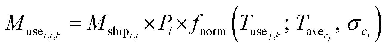
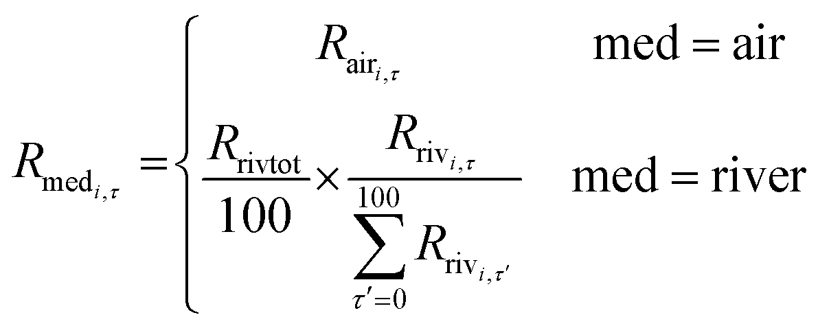
To obtain PECs for many different herbicides, one of the primary objectives of this research, we developed PeCHREM by using published information on pesticide formulations. The PeCHREM estimation scheme (Fig. 1) is divided into three phases. In the first phase, daily usage amounts of each herbicide formulation, including formulations of other types of pesticides also containing herbicides, were estimated for each prefecture under the following assumptions. All herbicide formulations applicable to paddy fields that were shipped into a prefecture were assumed to be completely used in that prefecture. All herbicide formulations were categorized into groups, and the temporal distribution of the used amounts of all herbicide formulations in the group was assumed to be the same in a given prefecture. These distributions were all assumed to follow a normal distribution. For all pesticides in one category, the temporal distribution of used amounts was assumed to be the same relative to a certain date (reference date) of farming work or a certain paddy rice growth phase, such as transplanting, rice plant heading, or harvest. These reference dates were the same in a given prefecture, but varied among prefectures. We categorized paddy herbicide formulations according to their registration information6 (see Sections 2.2 and 2.3 for details). We examined the relationship between the registration information on the herbicide formulations and actual usage records submitted by farmers before we decided on a categorization method (see Section 2.2 for details). In the second phase, we simulated temporal concentration changes of each herbicide in paddy fields and its emission rates (the proportion of the applied herbicide emitted per unit time) from paddy fields to rivers and the atmosphere based on the following assumptions. All herbicide formulations were assumed to be used in the recommended manner. If the recommended usage per unit area was a range, the arithmetic average of the lower and upper limits of the range was used. Temporal trends of herbicide concentration in paddy fields and the herbicide flux from paddy fields to the atmosphere followed a published fate model. The daily runoff amount of a herbicide in effluent water was assumed to be proportional to its concentration in paddy surface water. Influent and effluent water flows into and from paddy fields were assumed to be constant, and farming activities in paddy fields were ignored. The total runoff percentages of herbicides followed an empirical equation. We used the pesticide paddy field model (PADDY)20 as a fate model and an empirical equation suggested by Maru41 (see Section 2.4 for details). In the third phase, we calculated the daily emission amounts of each herbicide to rivers and the atmosphere in each tertiary mesh43 (1 km mesh) throughout Japan. Then we simulated environmental concentration changes of each herbicide throughout Japan by G-CIEMS by the following method. Only the emission of a herbicide from paddy fields to the atmosphere or to rivers was considered as an “emission” in the G-CIEMS model. Therefore, we did not calculate the fate of the target herbicide directly applied to paddy fields in the G-CIEMS model, but the fate of the herbicide deposited from the atmosphere onto paddy fields. The calculated concentrations of the herbicide in rivers are thus based on both runoff of the directly applied herbicide, which was simulated by the PADDY model, and the indirect effect via other media, as simulated by the G-CIEMS model (see Section 2.5 for details).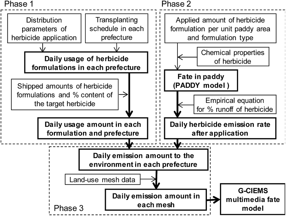 | ||
| Fig. 1 Scheme for estimating daily emissions of paddy herbicides to the environment in Japan (see Sections 2.2–2.5 for details). | ||
We used eqn (1) for the phase 1 calculation, eqn (2) for the phase 2 calculation, and eqn (3) for the phase 3 calculation.
 | (1) |
 | (2) |
 | (3) |
2.2 Categorization of the herbicide formulations
We collected 263 application records of pesticide formulations for paddy fields that were submitted by farmers to Japan Agricultural Cooperatives in Niigata (JA Zennoh Niigata)44 and Fukuoka (JA Munakata)45 prefectures (see Section 1 in the ESI† for details). Each application record was submitted by one farmer and included information such as transplantation and pesticide formulation application dates and all pesticide formulations used. Using these collected records, we constructed a set of records containing the name of a herbicide formulation, its use date, and the transplantation date. In the registration information for herbicide formulations, usage periods are usually indicated as, for example, “from 1 to 5 days after transplanting”.6 We compared the use dates of herbicide formulations in our record set among categories of herbicide formulations defined on the basis of their registration information, and then we selected a categorization method that was suitable for calculating the temporal distribution of use dates. To calculate the daily usage amounts of herbicide formulations from the total usage amount, we assumed that the transplanting day could be used as the reference date for calculating the distribution of use dates. From the registration information, we selected the first day of the suggested usage period after transplanting (hereafter, Property A), the last day of the suggested usage period after transplanting (Property B), and the highest leaf-growth stage of barnyard grass during the suggested usage period (Property C) for use in this comparison. For example, if the usage period of the herbicide formulation was given as “from 1 day after transplanting to leaf-growth stage 2.5 of barnyard grass, but only within 30 days after transplanting”, then Property A was 1, Property B was 30, and Property C was 2.5. If it was “from 15 to 50 days after transplanting”, then Property A was 15, Property B was 50, and Property C was no-information. We compared the relative dates, which were calculated by subtracting the transplantation date from the herbicide formulation use date (hereafter, relative dates of herbicide application) among herbicide formulations categorized by Property A, B, or C; both the relative date of application and the transplantation date were obtained from the set of application records.2.3 Herbicide usage amounts
Using the categorization results and the two related variables Tave and σ, along with the transplanting schedule in each prefecture,5 volumes of herbicide formulations shipped to each prefecture in Pesticide Year 2007 (October 2006 to September 2007),46 and the percentages of herbicides in each herbicide formulation,46 we calculated daily usage amounts of herbicides in each prefecture with eqn (1). Though the shipped volumes were from two years before our field survey, we could simulate the actual situation by using only the information obtainable before the field survey. For prefectures where double or early cropping is practiced,5 we divided the usage amounts of herbicide formulations into two schedules proportionally to the paddy field area;5 in other words, we calculated the daily usage amount and the related daily emission amounts separately for the two schedules by using eqn (1)–(3) and then added the results together to obtain the total daily emission amounts to the environment. In this study, we selected target herbicides in herbicide formulations suitable for rice in each target prefecture as judged from the registration information on the herbicide formulations; that is, rice was indicated as a target plant, and the target prefecture was in a region where the herbicide formulation is applied.2.4 Herbicide runoff ratios
Temporal concentration changes of herbicides in a paddy field were calculated from the application date to 100 days later with the PADDY model,20 in which simple processes are described by using parameters such as constant input and output water flows, volatilization to the atmosphere, adsorption and desorption onto solids, penetration into sediment layers, diffusion of pesticides in sediment layers, and elution of a pesticide formulation as a function of type (e.g., liquids, granules, or powder). In this study, elution of herbicide formulations was considered only in the case of powder and granular type formulations. In the PADDY model, parameter variations are described by simultaneous differential equations (see Section 2 in the ESI† for other model conditions). We used the Runge–Kutta–Gill method to solve these differential equations.We used the following empirical eqn (4) between the runoff percentage and herbicide solubility, which is based on field survey and lysimeter experiment data (see Section 3 in the ESI† for details).41
log10![[thin space (1/6-em)]](https://www.rsc.org/images/entities/char_2009.gif) R = −0.0819 + 0.286log10Cws R = −0.0819 + 0.286log10Cws | (4) |
2.5 Multimedia environmental fate model
The G-CIEMS model is a multimedia environmental fate model based on a Mackay level IV fugacity model, which depicts a non-equilibrium, unsteady-state, flow system. The basic compartments of the G-CIEMS model are air, freshwater (rivers and lakes), sediments of rivers and lakes, soils in seven land-use categories, forest canopy, and seawater and seafloor sediments.29 The spatio-temporal resolution of the G-CIEMS model is based on the GIS data used by the model. In this study, air grid cells with a resolution of about 5 km were used over the entire terrestrial land area. River and soil compartments shared the same river-network structure, which consisted of about 38000 unit catchments.47 The average length of a river segment in one unit catchment was 5.6 km, and the average area of a catchment segment was 9.7 km2.47 For simplicity, we selected the ordinary flow rate (i.e., the annual median flow rate) as the river flow condition.
Eqn (3) was used along with 1 km-mesh land-use data43 and prefectural data48 to calculate daily runoff into rivers and volatilization amounts into the atmosphere for each 1 km mesh. Then daily runoff amounts to a river segment from each catchment segment were calculated from the runoff amounts in 1 km meshes that overlapped catchment segments; the amounts were allocated proportionally to the ratio of the mesh area occupied by catchment segments to the total mesh area included in the G-CIEMS dataset.47 Daily volatilization amounts into each air grid were calculated from the 1 km-mesh volatilization amounts, because each air grid cell consisted of 25 of the 1 km-mesh cells. We used Microsoft Access® to construct a database file with several modules for the calculation; this file contained all required information about herbicide formulations, herbicides, transplanting schedules, and geography. We then used Microsoft Access® VBA to calculate emission datasets for each herbicide.
2.6 Target herbicides
We selected 25 target herbicides because they had high shipping volumes and because all the physico-chemical properties required for the prediction were available for them. The physico-chemical properties of the target herbicides were compiled from the literature49–52 and are listed in Table S2 in the ESI (see Section 3 in the ESI† for details). If the value of Henry's constant, which was calculated from molecular weight, solubility, and vapor pressure, was less than 0.01 m3 Pa mol−1, then a value of 0.01 was used for calculation stability. The degradation rate of herbicides in the atmosphere was fixed at 10−9 s−1, because available data were limited, and degradation in the atmosphere might not affect peak concentrations of herbicides in river water. The value of Henry's constant and the degradation rate in the atmosphere were used only by the G-CIEMS model.Many of the target herbicides may dissociate under environmental conditions. Therefore, both dissociated and non-dissociated species should be considered by environmental fate models. Franco and Trapp suggested a multimedia model for ionizable compounds.53 To correctly simulate the behavior of such compounds, physico-chemical properties under at least several pH conditions must be known. Because this information is hard to collect, we assumed that the compiled physico-chemical properties represented dissociated and non-dissociated species, considered as a whole, under environmental conditions. We also analyzed the possible influence of dissociated species on the G-CIEMS model's evaporation process and on related model calculations, because the evaporation rate can be strongly affected by the vapor pressure of a substance, for which the model assumed a non-dissociated species in equilibrium with its liquid or solid phase.54 We analyzed the possible influence of dissociated species on the actual evaporation process for three herbicides having relatively higher vapor pressures as follows. The fluxes of target herbicides from the surface water compartment to other compartments, including decomposition, were calculated for bentazon, benzobicyclon, and esprocarb.
2.7 Sampling and analytical method
River water samples were collected in clean amber glass bottles. In most cases, water samples were extracted by solid-phase extraction (SPE) within 2 days of collection; otherwise they were extracted within 4 days. All samples were kept at 4 °C until analysis by liquid chromatography-tandem mass spectrometry (LC/MS/MS). Just prior to SPE, each water sample (500 mL) was filtered through a glass fiber filter (GF/C, Whatman) and then acidified by the addition of hydrochloric acid (4 mol L−1, 100 μL). The filtrate was next loaded into an SPE cartridge (Oasis HLB plus, Waters) that had been preconditioned with 8 mL of acetone and 5 mL of pure water, and the target chemicals were extracted with 8 mL of acetone. The eluate was then evaporated to dryness under a gentle stream of nitrogen gas. The dried sample was reconstituted with 1 mL of acetonitrile for long-term storage at −20 °C. The reconstituted sample (200 μL) was mixed with 800 μL of methanol for LC/MS/MS analysis. Diuron-d6 was employed as an internal standard.LC/MS/MS measurements were performed by using an Agilent 1200 HPLC system equipped with an Agilent 6460 MS/MS (Agilent Technologies). The mass spectrometer was operated in electrospray ionization in selected reaction monitoring mode. A 1 μL sample of each extract was injected into a ZORBAX SB-C18 column (2.1 mm × 50 mm, 1.8 μm, Agilent Technologies). The LC mobile phases consisted of 5 mM ammonium acetate in water and 5 mM ammonium acetate in MeOH. The eluent gradient started at 10% methanol, followed by a 20 min ramp up to 90% methanol, and finalized by a 10 min hold. The flow rate was kept at 0.2 mL min−1. The collision energies, fragmentor voltages, and MS/MS parameters for the instrument were optimized individually for each analyte (see Table S3 in the ESI†); some values were obtained from published information.55 Three replicates of each recovery test were performed with pure water. This analytical method was developed with reference to the literature.55–57
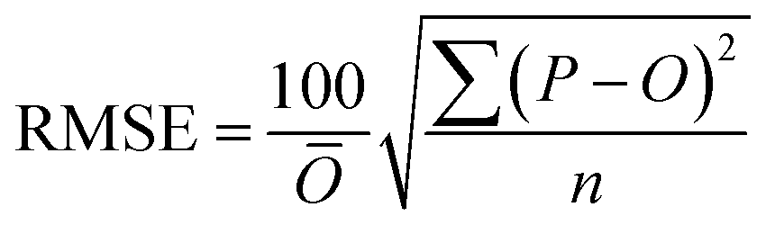
To compare the whole set of predicted and observed concentrations, we used two statistical indices, root mean square error (RMSE)58 and root mean square logarithmic error (RMSLE), as follows:
 | (5) |
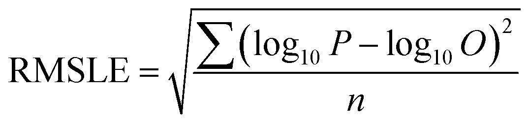 | (6) |
2.8 Sampling sites
Seven sites in Japan were selected (Fig. 2). Sampling site properties are listed in Table S4 in the ESI.† River waters were sampled between 13 April and 6 July 2009. The Hanamuro River was sampled twice a week, the Koise River was sampled once a week, and other rivers were sampled once every two weeks; the Yoshida, Usui, Kokai, Koise, and Hanamuro rivers were sampled again on 7 September 2009 to ascertain herbicide concentrations during a low-use period.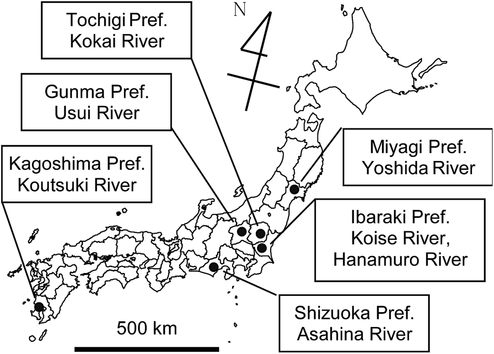 | ||
| Fig. 2 Sampling sites, including the name of each sampled river and the prefecture in which the site was located. | ||
3. Results and discussion
3.1 Categorization of herbicide formulations
We examined the relationships between the relative date of application of each herbicide formulation and Property A, B, and C values (Fig. S1 in the ESI†). The number of data obtained from the application records was 337 for Property A, 324 for Property B, and 329 for Property C. We found no relationship between the relative date of herbicide application and Property B, but the relative date of herbicide application tended to become higher as Property A or C values increased. We decided to use Property A to categorize herbicide formulations because there were enough records to cover the entire range of values (i.e., 0–20) only for Property A. Therefore, we grouped herbicide formulations into three categories based on the Property A value: Category A0 formulations had a Property A value of 0, Category A1 formulations had values of 1–5, and Category A2 formulations had values of 7–20. For each of these categories, the average and standard deviation of the relative date of herbicide application were calculated (Table S5 in the ESI†). In this calculation, herbicide formulations applied in nursery boxes were assigned to Category A0 because these herbicides were transferred to paddy fields during transplantation.We used the Kolmogorov–Smirnov method in the IBM SPSS Statistics 24 package to test the normality of the relative date distribution in each of the three categories. Only the dates in Category A2 were normally distributed (p > 0.05). Thus, we could not confirm the reliability of our categorization method because the number of the application records was insufficient. In the future, it will therefore be necessary to collect more application records of pesticide formulations.
3.2 Model predictions and comparisons with observations
We used the PeCHREM/G-CIEMS model to calculate spatio-temporal concentration changes of the 25 target herbicides throughout Japan and mapped the peak concentrations of each herbicide in river segments (Fig. 3). All herbicides were predicted to be present in all rivers, except butamifos in rivers in the northern island of Hokkaido. Comparison of the resulting maps showed that each herbicide had a unique spatial distribution. Thus, in Japan, where a herbicide concentration reaches its maximum value is different for each herbicide. Focusing on common characteristics of the spatial distributions, rivers with higher concentrations of herbicides tended to be located on plains, such as the Kokai, Koise, and Hanamuro rivers of the Kanto plain, because paddy fields are concentrated on plains.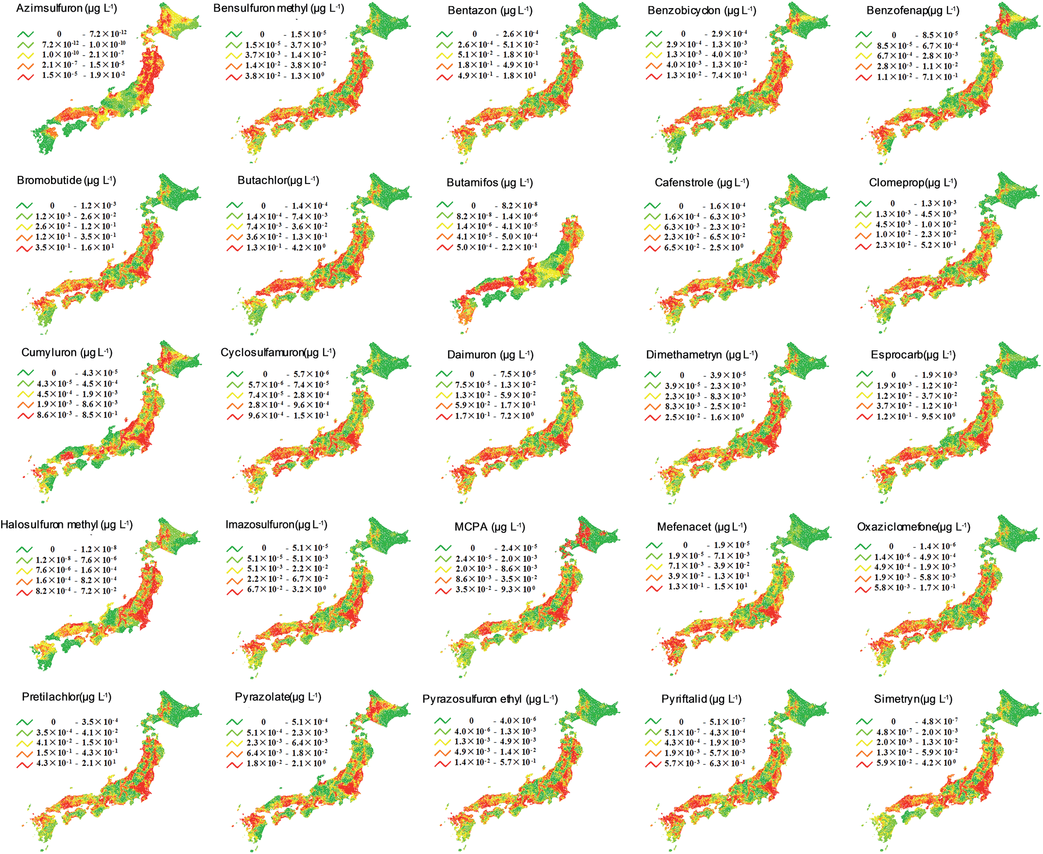 | ||
| Fig. 3 Maps of predicted peak concentrations of the 25 target herbicides. Rivers were divided into five groups with the number of rivers in each group depending on the peak concentration. | ||
We compared temporal changes in the herbicide PECs to observations for all 175 sampling site–herbicide combinations (Fig. 4). Many of the observed temporal trends were simple: concentrations first increased monotonically and then decreased monotonically. The degree to which the model predictions corresponded to observations varied: (a) predictions reliably reproduced observations during the entire survey period (e.g., F-Usui, Fig. 4); (b) the predicted and observed peak concentrations and peak dates corresponded to the observed peaks, but concentrations after the peak were predicted less accurately (e.g., N-Koise, Fig. 4); (c) only the peak date was reliably predicted (e.g., G-Yoshida, Fig. 4); and (d) the predicted concentration curve shape was similar to that of the observed data, but the peak concentration and peak date were not correctly predicted (e.g., Y-Kokai, Fig. 4).
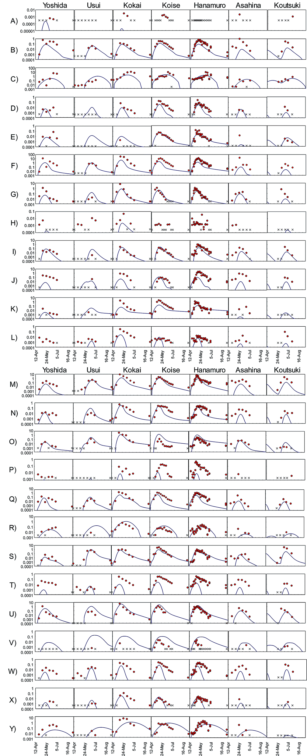 | ||
| Fig. 4 Comparisons of predicted (solid lines) with observed (dots) concentration changes in river water. Crosses indicate that no herbicide was detected and indicate the detection limit. The x axis shows the survey period dates (12 April to 12 September), and the y axis shows herbicide concentrations (μg L−1). The name of the sampled river is given at the top of each column, and the letters A–Y on the left represent herbicide names: (A) azimsulfuron, (B) bensulfuron methyl, (C) bentazon, (D) benzobicyclon, (E) benzofenap, (F) bromobutide, (G) butachlor, (H) butamifos, (I) cafenstrole, (J) clomeprop, (K) cumyluron, and (L) cyclosulfamuron, (M) daimuron, (N) dimethametryn, (O) esprocarb, (P) halosulfuron methyl, (Q) imazosulfuron, (R) MCPA, (S) mefenacet, (T) oxaziclomefone, (U) pretilachlor, (V) pyrazolate, (W) pyrazosulfuron ethyl, (X) pyriftalid, and (Y) simetryn. | ||
Herbicides were detected in river water in 166 of the 175 sampling site–herbicide combinations. We therefore evaluated the reliability of the model predictions by comparing the peak concentrations and peak dates between predictions and observations for these 166 combinations (Fig. 5). Comparisons among the rivers showed that the peak concentrations were overestimated in the Usui River and underestimated in the Kokai, Hanamuro, Asahina, and Koutsuki rivers. The peak concentration difference between predictions and observations was less than one order of magnitude in 109 combinations (i.e., in 66% of the 166 combinations). The predicted peak dates differed from the observed dates by less than two weeks in 131 combinations (i.e., in 79% of the 166 combinations). Herbicides were detected in at least three samples in 139 of the 175 sampling site–herbicide combinations. More than half of the observed concentrations differed from the corresponding predicted concentrations by less than one order of magnitude in 76 combinations (i.e., in 55% of the 139 combinations). All observed concentrations differed from the prediction by less than one order of magnitude in 20 combinations (i.e., in 14% of the 139 combinations). In the most reliable results, bromobutide in the Usui River (F-Usui) and benzofenap in the Koise River (E-Koise, Fig. 4), all of the observed concentrations were between half and twice the corresponding predicted concentrations.
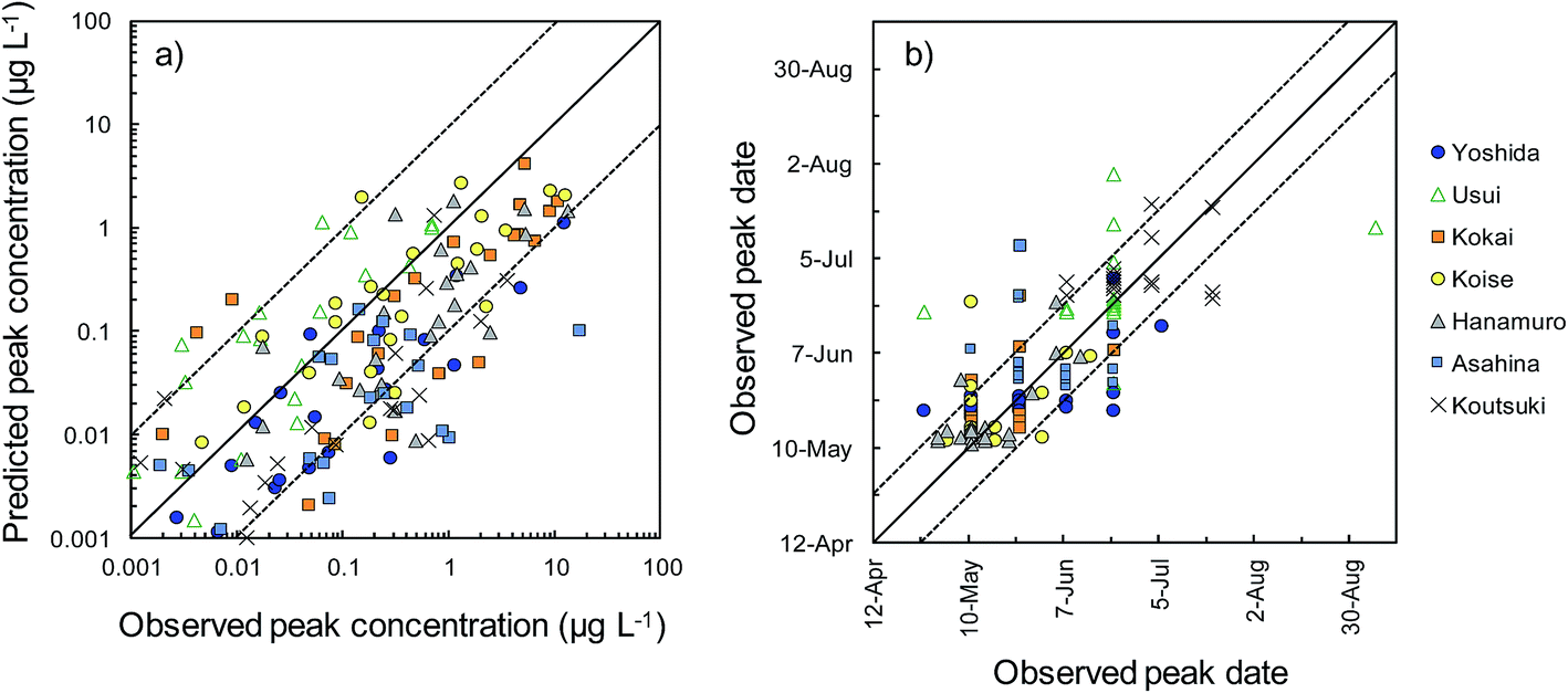 | ||
| Fig. 5 Relationships between predicted and observed (a) peak concentrations and (b) peak dates (when peak concentrations were predicted or observed). The solid lines indicate the lines of exact match, the dotted lines indicate (a) ten times higher or lower than the exact match and (b) two weeks earlier or later than the exact match. | ||
To compare the whole set of predicted and observed concentrations, we used two statistical indices, RMSE and RMSLE. The results are summarized in Table S6 in the ESI.† Predictions for several herbicides (e.g., benzobicyclon, benzofenap, and cumyluron) showed good agreement with observations during all observation periods.
The fluxes of target herbicides from the surface water compartment to other compartments, including decomposition, were calculated for bentazon, benzobicyclon, and esprocarb on 1 July, 1 June, and 1 June, respectively, when these herbicide concentrations in river water were consistently high. The percentages of the flux to the atmosphere relative to the total flux (outflow to the sea, settling to sediment, decomposition, and outflow to the atmosphere) were 0.004%, 0.05%, and 0.3% for bentazon, benzobicyclon, and esprocarb, respectively. Because dissociated species do not contribute to evaporation,53 the actual flux to the atmosphere would be lower than the calculated values. These results indicate, therefore, that the uncertainty of the evaporation process due to dissociated species had negligible influence on herbicide concentrations in river water. In the future, a more correct treatment of dissociated species and related pH conditions should be added to the model.
One possible cause for the underestimation of the concentrations of herbicides in rivers, especially during lower concentration periods, is that we used only percentages of the shipped volumes of herbicides contained in herbicide formulations applicable to paddy fields (summarized in Table 1). In the case of herbicides for which the “Volume applied to paddies” was less than 100%, the remaining percentage of the shipped volume was not considered in the model calculation. In addition, several of the target herbicides were included only in herbicide formulations applicable to paddy fields, but some of these herbicide formulations are applicable to both paddy and non-paddy fields. Therefore, some of the shipped volumes of herbicides in such formulations might have been used in non-paddy fields, and the model calculation results for these herbicides might be underestimations.
| Name of herbicide | Shipped volume (tons per year) | Volume applied to paddiesa (%) | Max. detected conc. (μg L−1) | Method detection limit (ng L−1) | No. of sites detected | No. of samples detected | Herbicide detection ratiob |
|---|---|---|---|---|---|---|---|
| a Percentage of shipped volume of the herbicide contained only in herbicide formulations applicable to paddy fields. b Ratio of the number of samples in which the herbicide was detected to the total number of samples (79). | |||||||
| Azimsulfuron | 0.08 | 100 | 0.0031 | 0.30 | 5 | 10 | 0.13 |
| Bensulfuron methyl | 45.51 | 100 | 1.0 | 0.46 | 7 | 72 | 0.91 |
| Bentazon | 318.49 | 100 | 11 | 2.5 | 7 | 76 | 0.96 |
| Benzobicyclon | 70.42 | 100 | 0.73 | 0.45 | 6 | 51 | 0.65 |
| Benzofenap | 57.93 | 100 | 0.15 | 0.13 | 6 | 47 | 0.59 |
| Bromobutide | 402.24 | 100 | 17 | 3.2 | 7 | 73 | 0.92 |
| Butachlor | 114.10 | 100 | 6.5 | 2.8 | 7 | 55 | 0.70 |
| Butamifos | 27.10 | 12 | 0.048 | 0.27 | 6 | 44 | 0.56 |
| Cafenstrole | 77.06 | 94 | 1.4 | 0.38 | 7 | 60 | 0.76 |
| Clomeprop | 78.69 | 100 | 0.49 | 0.37 | 7 | 37 | 0.47 |
| Cumyluron | 26.34 | 94 | 2.3 | 0.80 | 6 | 60 | 0.76 |
| Cyclosulfamuron | 160.41 | 1.6 | 0.30 | 0.68 | 7 | 64 | 0.81 |
| Daimuron | 285.56 | 100 | 9.0 | 0.94 | 7 | 76 | 0.96 |
| Dimethametryn | 15.47 | 100 | 0.48 | 0.19 | 7 | 72 | 0.91 |
| Esprocarb | 123.82 | 100 | 4.7 | 0.89 | 7 | 61 | 0.77 |
| Halosulfuron methyl | 6.63 | 16 | 0.54 | 2.0 | 6 | 52 | 0.66 |
| Imazosulfuron | 21.88 | 96 | 2.5 | 0.34 | 7 | 73 | 0.92 |
| MCPA | 80.42 | 98 | 0.73 | 2.9 | 7 | 58 | 0.73 |
| Mefenacet | 130.80 | 100 | 3.6 | 0.14 | 7 | 75 | 0.95 |
| Oxaziclomefone | 22.33 | 81 | 0.34 | 0.29 | 7 | 71 | 0.90 |
| Pretilachlor | 255.73 | 100 | 5.2 | 0.10 | 7 | 65 | 0.82 |
| Pyrazolate | 167.83 | 100 | 0.043 | 0.34 | 6 | 22 | 0.28 |
| Pyrazosulfuron ethyl | 10.32 | 91 | 0.28 | 0.26 | 7 | 71 | 0.90 |
| Pyriftalid | 8.65 | 100 | 0.11 | 0.45 | 7 | 42 | 0.53 |
| Simetryn | 60.88 | 100 | 4.5 | 2.6 | 6 | 63 | 0.80 |
3.3 Summary of the field surveys
At the seven sampling sites, the number of target herbicides detected ranged from 21 to 25 (Table S7 in the ESI†). The recovery rates of target herbicides are listed in Table S8 in the ESI.† Bentazon had a high recovery rate, and esprocarb had a low recovery rate. We did not correct quantitative concentrations by taking account of the recovery rates because we considered the effect of the difference in recovery rates on our conclusions to be negligible. Among the sampling sites, the Usui and Koutsuki river sites had relatively low site detection ratios (i.e., the ratio of the total number of herbicides detected at a site to the product of the number of samples collected at the site and the total number [25] of target herbicides), as well as lower maximum herbicide concentrations. In contrast, the detection ratios at the Hanamuro and Koise river sites were higher because of the higher sampling frequency at those sites, which caused a larger number of samples to be collected during the high-concentration period. This result indicates that multiple herbicides are used in many different places during the high-concentration period and are present in river waters at detectable levels.All target herbicides were detected in the field survey (Table 1). The shipped volumes and maximum concentrations of the 25 target herbicides were significantly correlated (Spearman's rank correlation coefficient (Rs) = 0.61, p < 0.01). More than half of the 25 target herbicides were only in herbicide formulations that are applicable to paddy fields, so these herbicides are probably applied mainly to paddy fields. These 16 herbicides showed a stronger significant correlation between the shipped volume and maximum concentration (Rs = 0.76, p < 0.01).
4. Conclusions
We developed PeCHREM, a method for estimating spatially and temporally variable emissions of various paddy herbicides from paddy fields to the environment, and then predicted day-to-day changes in environmental concentrations of 25 herbicides in Japan by using the multimedia environmental fate model G-CIEMS.29 The PeCHREM/G-CIEMS model results showed that the spatial distribution of peak concentrations in rivers was unique for each herbicide. We compared temporal changes in the predicted concentrations of target herbicides in rivers with the results of field surveys at seven river sites. In 20 of 139 sampling site–herbicide combinations in which herbicides were detected in at least three samples, all observed concentrations differed from the corresponding prediction by less than one order of magnitude. Comparison of the predicted results with the field survey results confirmed that the PeCHREM/G-CIEMS model could accurately predict the peak concentrations of paddy herbicides in river water as well as the dates on which the concentrations reached peak values. The peak concentration differences between predictions and observations were less than one order of magnitude in 66%, and the difference in peak dates was less than two weeks in 79%, of 166 sampling site–herbicide combinations. This model is applicable to many of the paddy herbicides used in Japan because all information about the target herbicides required for the prediction, except their physico-chemical properties, can be easily obtained from public websites and books. This model can therefore improve the efficiency and effectiveness of surveys by predicting peak concentrations and peak dates of many herbicides used in Japan.To develop the PeCHREM model, we devised a method for estimating the temporal distribution of the usage amounts of herbicide formulations in each prefecture by making several simple assumptions and by categorizing the herbicide formulations. Some of the parameters were calculated using data from application records submitted by farmers. There is still room for improvement with regard to the temporal distribution of the usage amounts of herbicide formulations and their categorization, because of the number of available application records is limited.
In this study, we focused on paddy herbicides because they all tend to be used intensively at rice transplanting time or within a certain number of days after transplanting.6 The concentrations of insecticides and fungicides used in paddy fields would probably be more difficult to predict. For more efficient and effective risk management, it will be necessary to improve the model so that the concentrations of these other pesticides can also be estimated. In addition, the pesticide ionization state (nonionic, cationic, or anionic) may also play an important role in pesticide behavior in water.59 Thus, an improved model method of calculating pesticide runoff ratios is also needed.
Many studies have investigated advanced ecological risk assessment. Forbes and Calow60 argued that a population growth rate analysis, instead of analyses of individual-level responses such as survival, reproduction, or growth, would allow more pragmatic ecological risk assessment. In addition, many studies have examined the use of data on time-varying exposure to pesticides in ecological risk assessment.60–64 Our model provided time-varying concentrations of pesticides to one of these studies.64 Therefore, our present model, or our improved future models, will also be able to contribute to advanced ecological risk assessments by providing reliable time-varying exposure data to ecological models.
Conflicts of interest
There are no conflicts of interest to declare.Acknowledgements
We would like to express our gratitude to J. Goukon from Miyagi Pref. Inst. Pub. Health & Env., Y. Imazu from Shizuoka Inst. Env. And Hygiene, R. Nagai from Kagoshima Pref. Inst. Env. Res. & Pub. Health, and H. Tomosaka from Gunma Nat. Coll. Tech. for their great support of our work.References
- R. B. Schäfer, P. C. von der Ohe, R. Kühne, G. Schüürmann and M. Liess, Environ. Sci. Technol., 2011, 45, 6167–6174 CrossRef PubMed.
- Ministry of Agriculture, Forestry and Fisheries, III Statistical Tables, http://www.maff.go.jp/j/tokei/census/afc/2005/pdf/eng_table.pdf, accessed 1 October 2012 Search PubMed.
- National Federation of Agricultural Cooperative Associations (Yamagata), Rice Cultivation in Shonai Plain (in Japanese), http://shonai.zennoh-yamagata.or.jp/kome/images/kome-file.pdf, accessed 29 September 2017 Search PubMed.
- National Federation of Agricultural Cooperative Associations (Yamaguchi), Cultivation Calendar of paddy-field rice (in Japanese), https://www.ja-syunan.or.jp/pdf/nogyo/koyomi.pdf, accessed 29 September 2017 Search PubMed.
- Statistics Department, Minister's Secretariat of the Ministry of Agriculture, Forestry and Fisheries, Crop condition of paddy field rice as of August 15 (in Japanese), 2007 Search PubMed.
- Food and Agricultural Materials Inspection Center, Database of Pesticide Registration Information (in Japanese), http://www.acis.famic.go.jp/ddownload/index.htm, 20 February 2008 Search PubMed.
- T. Nagai, K. Inao and T. Horio, J. Pestic. Sci., 2008, 33, 393–402 CrossRef CAS.
- U.S. Environmental Protection Agency, Guidelines for Ecological Risk Assessment, EPA/630/R-95/002F, Washington, DC, 1998 Search PubMed.
- European Communities, Technical Guidance Document on Risk Assessment. Part II. EUR 20418 EN/2, 2003 Search PubMed.
- T. Nagai, J. Pestic. Sci., 2017, 42, 124–131 CrossRef.
- Ministry of Agriculture, Forestry and Fisheries, Data Requirements for Supporting Registration of Agricultural Chemicals (No. 12-8147), 2000 Search PubMed.
- Ministry of the Environment, I. Concept of Calculating the Predicted Environmental Concentration for Ecological Risk Assessment (in Japanese), http://www.env.go.jp/water/sui-kaitei/kijun/concept.pdf, accessed 3 October 2017 Search PubMed.
- Ministry of the Environment, Comprehensive survey on pesticide residues (in Japanese), https://www.env.go.jp/water/dojo/noyaku/report2/index.html, accessed 2 October 2017 Search PubMed.
- S. Yachi, T. Nagai and K. Inao, Jpn. J. Pestic. Sci., 2017, 42, 1–9 CrossRef.
- S. H. Vu, S. Ishihara and H. Watanabe, Pest Manage. Sci., 2006, 62, 1193–1206 CrossRef CAS PubMed.
- T. Iwakuma, H. Shiraishi, S. Nohara and K. Takamura, Chemosphere, 1993, 27, 677–691 CrossRef CAS.
- L. Comoretto, B. Arfib, R. Talva, P. Chauvelon, M. Pichaud, S. Chiron and P. Hoehener, Environ. Pollut., 2008, 151, 486–493 CrossRef CAS PubMed.
- S. Hatakeyama and H. Shiraishi, Environ. Toxicol. Chem., 1998, 17, 687–694 CrossRef.
- S. Ebise and H. Kawamura, J. Jpn. Soc. Water Environ., 2006, 29, 705–713 CrossRef CAS.
- K. Inao and Y. Kitamura, Pestic. Sci., 1999, 55, 38–46 CrossRef CAS.
- S. E. Jorgensen, J. C. Marques and P. M. Anastacio, Ecol. Model., 1997, 104, 205–213 CrossRef CAS.
- E. Capri and Z. W. Miao, Agronomie, 2002, 22, 363–371 CrossRef.
- Z. W. Miao, M. J. Cheplick, M. W. Williams, M. Trevisan, L. Padovani, M. Gennari, A. Ferrero, F. Vidotto and E. Capri, J. Environ. Qual., 2003, 32, 2189–2199 CrossRef CAS PubMed.
- A. Di Guardo, D. Calamari, G. Zanin, A. Consalter and D. Mackay, Chemosphere, 1994, 28, 511–531 CrossRef CAS.
- Y. Nakano, T. Yoshida and T. Inoue, Water Res., 2004, 38, 3023–3030 CrossRef CAS PubMed.
- A. Pistocchi, D. A. Sarigiannis and P. Vizcaino, Sci. Total Environ., 2010, 408, 3817–3830 CrossRef CAS PubMed.
- J. Boulange, H. Watanabe, K. Inao, T. Iwafune, M. H. Zhang, Y. Z. Luo and J. Arnold, J. Hydrol., 2014, 517, 146–156 CrossRef CAS.
- S. Stehle, J. M. Dabrowski, U. Bangert and R. Schulz, Sci. Total Environ., 2016, 545, 171–183 CrossRef PubMed.
- N. Suzuki, K. Murasawa, T. Sakurai, K. Nansai, K. Matsuhashi, Y. Moriguchi, K. Tanabe, O. Nakasugi and M. Morita, Environ. Sci. Technol., 2004, 38, 5682–5693 CrossRef CAS PubMed.
- D. Mackay and S. Paterson, Environ. Sci. Technol., 1991, 25, 427–436 CrossRef CAS.
- M. MacLeod, D. G. Woodfine, D. Mackay, T. McKone, D. Bennett and R. Maddalena, Environ. Sci. Pollut. Res., 2001, 8, 156–163 CrossRef CAS PubMed.
- D. G. Woodfine, M. MacLeod, D. Mackay and J. R. Brimacombe, Environ. Sci. Pollut. Res., 2001, 8, 164–172 CrossRef CAS PubMed.
- K. Kawamoto, M. MacLeod and D. Mackay, Chemosphere, 2001, 44, 599–612 CrossRef CAS PubMed.
- M. Scheringer, F. Wegmann, K. Fenner and K. Hungerbuhler, Environ. Sci. Technol., 2000, 34, 1842–1850 CrossRef CAS.
- U. Schenker, M. Scheringer and K. Hungerbuhler, Environ. Sci. Pollut. Res., 2007, 14, 145–152 CrossRef CAS PubMed.
- R. van Zelm, M. A. J. Huijbregts and D. van de Meent, Int. J. Life Cycle Assess., 2009, 14, 282–284 CrossRef.
- N. Kehrein, J. Berlekamp and J. Klasmeier, Environ. Model. Software, 2015, 64, 1–8 CrossRef.
- K. E. Kapo, P. C. Deleo, R. Vamshi, C. M. Holmes, D. Ferrer, S. D. Dyer, X. H. Wang and C. White-Hull, Integrated Environ. Assess. Manag., 2016, 12, 782–792 CrossRef PubMed.
- M. Oyamada and S. Kuwatsuka, J. Pestic. Sci., 1988, 13, 99–105 CrossRef CAS.
- S. Amano, T. Kagiya and T. Katami, J. Environ. Chem., 2001, 11, 785–792 CrossRef CAS.
- S. Maru, J. Pestic. Sci., 1993, 18, S135–S143 CrossRef CAS.
- N. Suzuki, K. Murasawa, K. Nansai, T. Sakurai, Y. Moriguchi, K. Tanabe, O. Nagasugi and M. Morita, River networking database for geo-referenced fate modeling of Japanese river, Research Report from the National Institute for Environmental Studies, Japan, R-179(CD)-2003, 2003 Search PubMed.
- National Land Information Division, National and Regional Policy Bureau, Ministry of Land, Infrastructure, Transport and Tourism, National Land Numerical Information: Land utilization tertiary mesh Data 1997 Tokyo Datum, http://nlftp.mlit.go.jp/ksj/jpgis/datalist/KsjTmplt-L03-a.html, 2 December 2008 Search PubMed.
- Japan agricultural cooperative in Niigata prefecture (JA Zennoh Niigata), Operation records of farming (in Japanese), http://www.nt.zennoh.or.jp/, accessed 27 July 2008 Search PubMed.
- Japan agricultural cooperative in Munakata city (JA Munakata), Operation records of farming (in Japanese), http://www.ja-munakata.or.jp/, accessed 24 July 2008 Search PubMed.
- Japan Plant Protection Association, Noyaku Yoran (Yearbook of Agricultural Chemicals) (in Japanese), Japan Plant Protection Association, Tokyo, 2008 Search PubMed.
- N. Suzuki, G-CIEMS Model (in Japanese), http://www.nies.go.jp/rcer_expoass/gciems/gciems.html, accessed 15 February 2010 Search PubMed.
- National Land Information Division, National and Regional Policy Bureau, Ministry of Land, Infrastructure, Transport and Tourism, National Land Numerical Information: Administrative Zones Data 2005 JGD2000, http://nlftp.mlit.go.jp/ksj/jpgis/datalist/KsjTmplt-N03.html, 2 December 2008 Search PubMed.
- Japan Plant Protection Association, Noyaku Handobukku (Agricultural Chemical Handbook) 2005 (in Japanese), Japan Plant Protection Association, Tokyo, 2005 Search PubMed.
- C. D. S. Tomlin, The E-pesticide Manual: A World Compendium, Version 4.2, British Crop Protection Council, Hampshire, 2009 Search PubMed.
- The Food Safety Commission of Japan, Risk Assessment Reports of Pesticides (In Japanese), http://www.fsc.go.jp/senmon/nouyaku/index.html, accessed 6 January 2011 Search PubMed.
- J. Kanazawa, Noyaku no Kankyotokusei to Dokuseidetashu (Data on environmental property and toxicity of pesticide) (in Japanese), Godo Publishers, Tokyo, 1996 Search PubMed.
- A. Franco and S. Trapp, Environ. Toxicol. Chem., 2010, 29, 789–799 CrossRef CAS PubMed.
- A. Delle Site, J. Phys. Chem. Ref. Data, 1997, 26, 157–193 CrossRef.
- National Institute for Environmental Studies, Aquatic organisms and their environments in irrigation ponds (in Japanese), Report from the National Institute for Environmental Studies, Japan, F-116–2011, 2011 Search PubMed.
- I. R. Pizzutti, A. de Kok, R. Zanella, M. B. Adaime, M. Hiemstra, C. Wickert and O. D. Prestes, J. Chromatogr. A, 2007, 1142, 123–136 CrossRef CAS PubMed.
- T. Iwafune, K. Inao, T. Horio, N. Iwasaki, A. Yokoyama and T. Nagai, J. Pestic. Sci., 2010, 35, 114–123 CrossRef CAS.
- A. Infantino, T. Pereira, C. Ferrari, M. J. Cerejeira and A. Di Guardo, Chemosphere, 2008, 70, 1298–1308 CrossRef CAS PubMed.
- M. Arias-Estevez, E. Lopez-Periago, E. Martinez-Carballo, J. Simal-Gandara, J. C. Mejuto and L. Garcia-Rio, Agric. Ecosyst. Environ., 2008, 123, 247–260 CrossRef CAS.
- V. E. Forbes and P. Calow, Philos. Trans. R. Soc. London, Ser. B, 2002, 357, 1299–1306 CrossRef PubMed.
- J. J. T. I. Boesten, H. Koepp, P. I. Adriaanse, T. C. M. Brock and V. E. Forbes, Ecotoxicol. Environ. Saf., 2007, 66, 291–308 CrossRef CAS PubMed.
- K. H. Reinert, J. A. Giddings and L. Judd, Environ. Toxicol. Chem., 2002, 21, 1977–1992 CrossRef CAS PubMed.
- T. Nagai, Hum. Ecol. Risk Assess., 2014, 20, 641–657 CrossRef CAS.
- T. I. Hayashi, Y. Imaizumi, H. Yokomizo, N. Tatarazako and N. Suzuki, Environ. Toxicol. Chem., 2016, 35, 233–240 CrossRef CAS PubMed.
Footnotes |
| † Electronic supplementary information (ESI) available. See DOI: 10.1039/c7em00517b |
| ‡ Author contributions: S. Serizawa helped to develop the analytical method, but she is unaware that this paper is being submitted for publication as we have no contact details for her. Therefore, she does not take any responsibility for the contents. |
| This journal is © The Royal Society of Chemistry 2018 |