Using time-resolved photoelectron spectroscopy to unravel the electronic relaxation dynamics of photoexcited molecules

Abstract

Time-resolved photoelectron spectroscopy measurements combined with quantum chemistry and dynamics calculations allow unprecedented insight into the electronic relaxation mechanisms of photoexcited molecules in the gas-phase. In this Tutorial Review, we explain the essential concepts linking photoelectron spectroscopy measurements with electronic structure and how key features on the potential energy landscape are identified using quantum chemistry and quantum dynamics calculations. We illustrate how time-resolved photoelectron spectroscopy and theory work together using examples ranging in complexity from the prototypical organic molecule benzene to a pyrrole dimer bound by a weak N–H⋯π interaction and the green fluorescent protein chromophore.

---

Helen H. Fielding

Helen Fielding graduated with a DPhil in Physical Chemistry from the University of Oxford in 1992. She then carried out postdoctoral research in the Department of Physics at the University of Amsterdam before becoming a Lecturer in Physical Chemistry at King's College London in 1994. She moved as a Professor to University College London in 2003, where she is currently Head of Physical Chemistry. Her research is focussed on understanding and controlling the fate of electronically excited states of molecules formed following the absorption of ultraviolet light. She is interested in systems ranging in complexity from small organic molecules to photoactive protein chromophores and molecular motors.

Graham A. Worth

Graham Worth obtained a DPhil in Chemistry at the University of Oxford in 1992. After working as a postdoctoral researcher in Heidelberg, first at the EMBL then at the University, he became a Research Fellow at King's College London in 2000. He then moved to the University of Birmingham in 2005, where he became a Professor in 2013. In 2016, he moved to University College London to become Professor of Computational Chemistry. His main research is focussed on the development of efficient algorithms for solving the time-dependent Schrödinger equation and its application to fundamental processes in polyatomic molecules. A particular interest is the description of photo-excited molecular dynamics and light-matter interaction.

---

Key learning points

• Use of time-resolved photoelectron spectroscopy to track excited state dynamics

• Use of quantum chemistry and quantum dynamics calculations to characterise potential energy landscapes

• Calculation of parameters related to experimental observables

• Interpretation of time-resolved photoelectron spectra of molecules

1 Introduction

There is considerable interest in the electronic relaxation of molecules following excitation with ultraviolet (UV) light, both from a fundamental point of view and as a result of its significance in biology and technology; important examples include photosynthesis, vision, photodamage, phototherapies, imaging and photovoltaics. In terms of studying the electronic relaxation mechanisms of the molecular units that lie at the heart of the complex systems involved in these processes, it is recognised that experiments on isolated molecules in the gas-phase, free from interactions with a solvent or protein micro-environment, allow the intrinsic properties of a molecule to be studied in fine detail. Comparing the dynamics of an isolated molecule with those of the corresponding molecular unit in its natural environment makes it possible to disentangle the contribution from the interaction between the molecule and its micro-environment. Such a bottom-up approach provides an important starting point for studying complex systems. In this tutorial review, we explain how time-resolved photoelectron spectroscopy and theory work together to allow us to gain particularly detailed insight into the electronic relaxation mechanisms of photoexcited molecules in the gas-phase.

When a molecule absorbs ultraviolet (UV) light, it is promoted to an electronically excited state in which the nuclei are no longer in their equilibrium positions. The resulting excess vibrational energy is subsequently redistributed within the molecule in a variety of ways. The coupling between vibrational modes leads to intramolecular vibrational energy redistribution (IVR), typically on a timescale of 10⁻¹²–10⁻¹⁰ s. The molecule may then relax back to the ground electronic state by emitting a photon; the timescales for fluorescence, from a singlet excited state to a singlet ground state, or phosphorescence, from a triplet excited state to a singlet ground state, are approximately 10⁻¹⁰–10⁻⁷ s and 10⁻⁶–1 s, respectively. Non-radiative electronic relaxation processes often compete with these radiative electronic relaxation processes, e.g., an excited singlet state may undergo internal conversion (IC) to a lower lying singlet state, on a timescale of 10⁻¹⁴–10⁻¹¹ s, or it may undergo intersystem crossing (ISC) to a lower lying triplet state, typically on a timescale of 10⁻¹⁰–10⁻⁸ s, depending on the strength of the coupling between the states. The electronic energy lost during IC or ISC is transferred to nuclear degrees of freedom. These photophysical processes are all illustrated in Fig. 1.

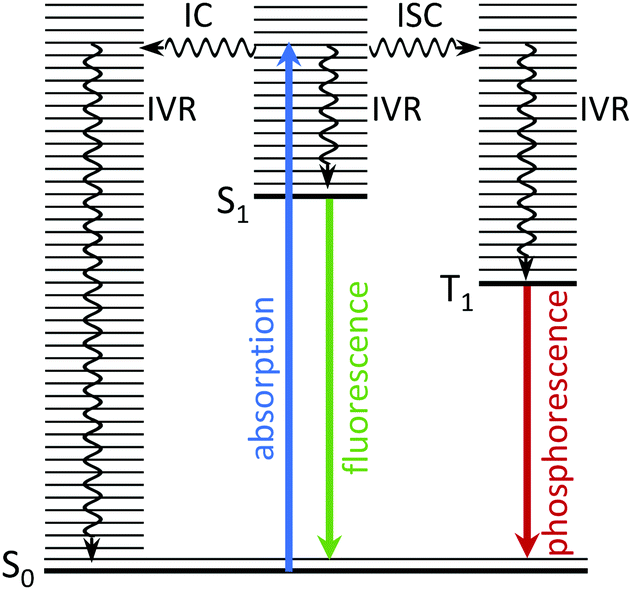Fig. 1 Jablonski diagram illustrating the photophysical relaxation pathways open to a molecule following photoexcitation from S₀ to vibrationally excited levels of S₁.

Alternatively, the molecule may undergo a photochemical reaction in its excited electronic state, e.g. dissociation, isomerisation, electron-transfer or proton-transfer, before relaxing back to the ground electronic state. These processes typically take place on timescales of 10⁻¹⁵–10⁻¹² s. Although radiative processes almost always take place at, or near to, minimum energy configurations on the excited potential energy surface, non-radiative processes almost always take place at, or near to, molecular configurations in which two or more electronic states are degenerate, known as a conical intersection (CI). A CI seam between two electronic states is illustrated in Fig. 2.

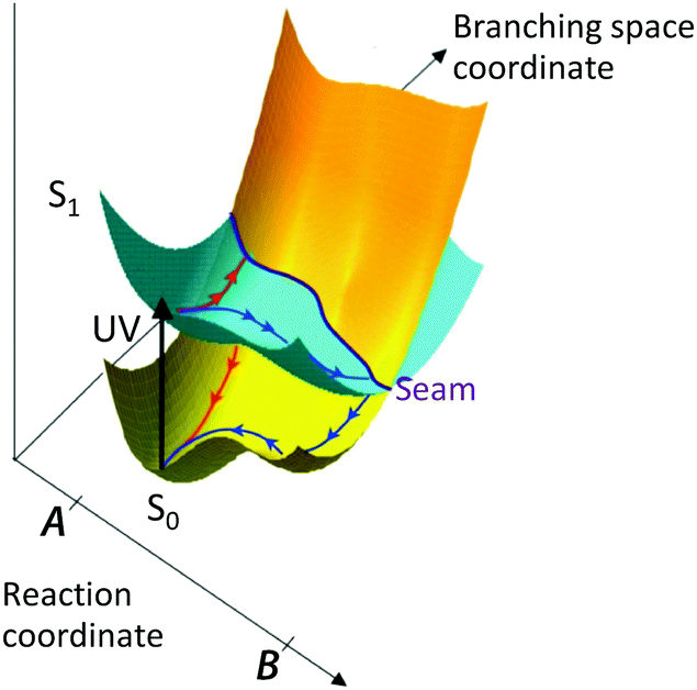Fig. 2 Schematic illustration of a conical intersection seam between excited and ground electronic states in a simple photochemical reaction (adapted from ref. 1 with the permission of the author). Following UV photoexcitation, there are two possible reaction coordinates that take population to different regions of the conical intersection seam where it undergoes internal conversion back to the ground electronic state (red path) or photochemistry on the excited state before returning to the ground electronic state (blue path).

The outcome of a photoreaction depends on the shapes of the potential energy surfaces and the molecular configurations where the electronic relaxation occurs on the CI seam. There are two limiting cases: the reaction path may cross through the seam near the reactants, which corresponds to a photophysical process, or a reaction may occur on the excited state and the reaction path crosses the seam near the products. In order to understand how energy flows in molecules following the absorption of a photon, it is necessary to understand the relationship between the molecular structure, the topography of the potential energy landscape and the outcome of a photochemical reaction, i.e. the structure–dynamics–function relationship. This requires experimental measurements to track the excited state dynamics of molecules and theory to determine the electronic energies and nuclear geometries of key features on the potential energy landscape, e.g., conical intersections and avoided crossings, minima and transition states, and parameters related to experimental observables. The aim of this tutorial review is to explain how to combine time-resolved photoelectron spectroscopy measurements with quantum chemistry and quantum dynamics calculations to unravel the relaxation mechanisms of photoexcited molecules in the gas-phase.

2 The experimental toolkit

2.1 Time-resolved photoelectron spectroscopy

Time-resolved photoelectron (TRPES) spectroscopy is ideally suited to tracking electronic relaxation following photoexcitation because it involves the direct measurement of evolving electronic and vibrational structure. For excellent detailed reviews of TRPES, the reader is referred to ref. 2–4.

In the independent electron approximation, photoionisation of an outer electron occurs without any reorganisation of the remaining electrons – this is known as the ‘molecular orbital’ or Koopmans picture. Measuring the electron kinetic energy (eKE) distribution of photoelectrons emitted following photoionisation allows us to determine the electron binding energy (eBE) of the molecular orbital from which the electron is ionised, with respect to the electronic state of the cation that is left behind, using eBE = hν − eKE where hν is the photon energy. The propensity for conserving vibrational energy during photoionisation, at least in rigid molecules that do not undergo large amplitude motions, also allows us to use the Franck–Condon distribution of photoelectron eKEs to identify non-resonant and resonant two-photon ionisation processes (Fig. 3).

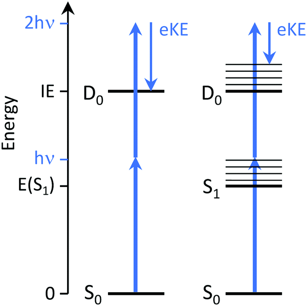Fig. 3 Schematic energy level diagram illustrating UV photoelectron spectroscopy of a molecule. Left: Direct photoionisation from S₀ to the D₀ continuum gives eKE = 2hν − IE. Right: Indirect photoionisation following photoexcitation of S₁ with excess vibrational energy E_v = hν − E(S₁) gives eKE = hν − [IE − E(S₁)].

Measuring the photoelectron angular distribution (PAD) as well as the eKE distribution allows us to obtain additional information about the molecular orbital from which the electron is ionised.⁵ As the electron leaves the molecule, it scatters from the molecular potential and the scattering wave function reflects the electronic and nuclear configurations of the neutral molecule at the moment of ionization. There is a requirement that the direct product of the irreducible representations of the free electron wave function (Γ_e⁻), the electronic state of the cation (Γ_M⁺), the transition dipole moment operator (Γ_μ) and the electronic state of the neutral molecule (Γ_M) contains the totally symmetric irreducible representation of the molecular point group (Γ_s), i.e. Γ_e⁻ ⊗ Γ_M⁺ ⊗ Γ_μ ⊗ Γ_M ⊂ Γ_s. The PAD is measured in the laboratory frame relative to the electric field vector of the photoionising laser and reflects the electronic symmetry of the neutral molecule and the symmetries of the contributing molecular frame transition dipole moment components. Since the relative contributions of the molecular frame transition dipole moments are determined geometrically by the orientation of the molecule relative to the ionising laser field polarisation, the form of the measured PAD will reflect the distribution of molecular axes.

In a TRPES experiment, an ultrashort pump laser pulse (typically ∼100 fs) promotes a molecule to an excited electronic state and a second ultrashort probe laser pulse then ionises the evolving excited state of the molecule (Fig. 4). The wavelength of the probe pulse is usually selected to allow access to as much of the ionisation continuum as possible whilst minimising absorption to excited electronic states to avoid the possibility of probe–pump dynamics complicating the TRPES. The eKE distributions (and PADs) are then measured at a series of precisely timed pump–probe time intervals. One of the advantages of TRPES over pump–probe methods such as transient absorption spectroscopy or time-resolved fluorescence spectroscopy, is that ionisation is always an allowed process because the selection rules are relaxed as a result of the range of possible symmetries of the outgoing electron, i.e. there are no optically dark states in photoionisation.

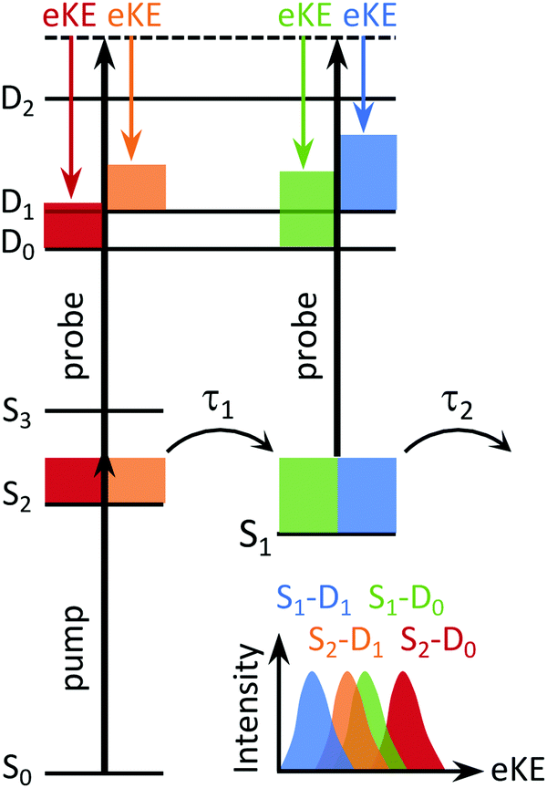Fig. 4 Schematic energy level diagram showing the four lowest, singlet states of a neutral molecule (S₀, S₁, S₂, S₃) and the three lowest doublet states (D₀, D₁, D₂) of the corresponding molecular cation. The coloured blocks represent the excess vibrational energy following photoexcitation of S₀. The timescales for S₂/S₁ IC and S₁/S₀ IC are marked τ₁ and τ₂, respectively. As a result of the propensity for vibrational energy to be conserved during photoionisation, we would expect the photoelectrons resulting from ionisation of S₂ to have higher eKE than those arising from ionisation of S₁, for each electronic state of the cation. Different electronically excited states may also be projected onto different electronic states of the cation, resulting in overlapping bands in the photoelectron spectrum (bottom).

2.2 Molecular sources

In order to make TRPES measurements of isolated molecules in the gas-phase, an expansion into a vacuum chamber is required to ensure the high vacuum requirements (<10⁻⁶ mbar) of electron detectors is met. A common way of generating a collimated, high density molecular beam is to seed the vapour of a liquid or solid sample in an inert carrier gas, such as He or Ar, at high pressure and to allow this to expand (continuously or pulsed) into the vacuum through a nozzle with a 50–500 μm hole, separated from the laser-molecule interaction region by a skimmer with a diameter of a few mm. Such molecular beams have small transverse velocity and very low velocity spread in the propagation direction and the molecules are vibrationally and rotationally cold, thus simplifying spectra by reducing the number of quantum states that are accessible in the photoexcitation process. Although the liquid or solid sample can be heated to increase the vapour pressure, and hence the number density, many large molecules are not particularly volatile and decompose before sufficiently high vapour pressure can be achieved. Laser desorption from a surface is a reasonably gentle method of transferring large neutral molecules into a vacuum. Alternatively, electrospray ionisation (ESI) is a very effective method for transferring very large molecules, including whole proteins, into the gas-phase in their deprotonated anionic or protonated cationic forms. In ESI, the ions in solution are pushed through the tip of a syringe needle held at high potential relative to the entrance of a mass-spectrometer. A more recent development is TRPES of liquid samples,⁶ which involves using a quartz glass capillary with a diameter of a few tens of μm to deliver a continuous flow of liquid to the laser-molecule interaction region. Comparing TRPES of isolated molecules in the gas-phase with analogous measurements of molecules in their natural aqueous or protein environments promises to be a particularly powerful way of disentangling the contribution to the dynamics from the interactions between the molecule and its micro-environment, and is the approach that we have developed in our laboratory.

2.3 Photoelectron spectrometers

There are several techniques for measuring photoelectron spectra, the most popular of which are based on velocity map imaging (VMI) or time-of-flight (TOF) methods. VMI allows both the eKE distribution and PAD to be measured simultaneously. VMI uses static electric fields to project the 3D photoelectron momentum distribution created in the laser-molecule interaction region onto a 2D position-sensitive electron detector, which usually comprises a microchannel plate, a phosphor screen and a charge-coupled device (CCD) camera. The original 3D photoelectron momentum distribution can be reconstructed from the 2D image using an inversion algorithm. TOF spectrometers measure the eKE distribution by analysing the time taken for the electrons to travel from the laser-molecule interaction region to an electron detector. A commonly employed TOF spectrometer is the magnetic bottle photoelectron spectrometer in which photoelectrons created in the laser-molecule interaction region are guided in a magnetic field toward the electron detector, which is usually a microchannel plate. TOF spectrometers can be constructed to have high energy resolution and are the spectrometers of choice for liquid samples because it is relatively straightforward to keep the liquid vapour away from the electron detector.

2.4 Analysis of TRPES measurements

For each excitation wavelength, the total integrated photoelectron signal and a set of photoelectron images or spectra are recorded at a selection of pump–probe delays. Time-zero and the Gaussian cross-correlation function representing the cross-correlation of the pump and probe laser pulses, g(t), may be obtained externally by frequency-mixing the pump and probe laser pulses in nonlinear crystals, or in the laser-molecule interaction region by using two-colour, non-resonant, multiphoton (1 + 1′) ionisation of a gaseous system. Alternatively, the integrated photoelectron signal can be fit to sums of exponentially decaying profiles convoluted with a Gaussian cross-correlation function,where c_i is the intensity of the ith decay with 1/e decay time τ_i.

To extract decay times from a set of time-resolved photoelectron spectra, the integrated areas of the photoelectron spectra recorded at each pump–probe delay are scaled to the intensity of the integrated photoelectron signal at that pump–probe delay and the set of scaled photoelectron spectra are fit to the expression

The coefficients C_i(eKE) represent the contribution of the ith decay at a given eKE. Positive values of C_i(eKE) represent exponential decay at timescale τ_i and negative values represent exponential growth at τ_i. Varying the time-zero values allows the robustness of the fit to be tested and the confidence limits for the FWHM and τ_i to be determined.

To a first approximation, the decay associated spectra, C_i(eKE), can be understood using conservation of energy. Assuming the excess vibrational energy for a given electronic state E_vib = hν_pump – E(S_n) is conserved during photoionisation, eKE = hν_probe – [E(D_n) – E(S_n)]. Thus, knowing the vertical excitation energies of the electronically excited states of the neutral molecule and the ionisation energies and propensities for ionisation from each electronically excited state to each continuum (Section 3), allows us to assign the different components of the photoelectron spectra to different regions of the excited state potential energy surface.

Qualitative insight into the nature of the molecular orbitals from which the electron is photoionised can also be obtained from PADs which, for a two-photon pump–probe experiment, may be fit to the expression

I(θ) = a[1 + β₂P₂(cos θ) + β₄P₄(cos θ)], (3)

where I(θ) is the probability of photoelectron emission at a particular angle θ, defined as the angle between the laser polarisation and the velocity vector of the photoelectron. P_n(cos θ) are the nth order Legendre Polynomials, β_n are the asymmetry parameters and a is a normalisation constant. The two limiting values of β₂ are +2 and −1, corresponding to photoelectron emission predominantly parallel (cos² θ distribution) and perpendicular (sin² θ distribution) to the laser polarisation, respectively. Unless there is a continuum resonance, states that give rise to photoelectrons with different anisotropies can be assumed to have different electronic character and, in general, a negative β₂ can be attributed to photoionisation from an orbital with p or π character and a positive β₂ can be attributed to photoionisation from an orbital with s or σ character.

3 The computational toolkit

To interpret TRPES measurements requires quantum chemistry calculations to determine the electronic energies and nuclear geometries of key features on the potential energy landscape as well as ionisation energies and propensities. To interpret the timescales determined from TRPES measurements and understand where the energy is flowing following photoexcitation requires quantum dynamics calculations.

3.1 Quantum chemistry calculations

There are three important types of critical points on the potential energy landscape and they are differentiated by derivatives of the potential energy with respect to displacements of nuclear coordinates. Potential minima, corresponding to stable species, are characterised by all the first derivatives being zero and all the second derivatives being positive. Saddle points, corresponding to transition states, are characterised by all the first derivatives being zero and all the second derivatives being positive except one. Conical intersections form a seam of points (Fig. 2) where two potential surfaces meet. Moving away from this seam in two particular directions, known as the gradient difference and derivative coupling vectors (g and h), the intersection has the topography of a double cone. The properties of conical intersections have been the subject of a number of books and reviews.^7,8 Asymptotes, corresponding to dissociation channels, may also be important.

To calculate the potential energy at a given nuclear geometry requires us to solve the electronic Schrödinger equation at that nuclear geometry. This can be achieved using a quantum chemistry program, such as Gaussian, Molpro, Qchem or Molcas. A method and a basis set must be selected that balance computational resources and accuracy.

The method defines the way in which the wavefunction is represented and the level of approximation used to solve the Schrödinger equation. Methods can be divided into two classes: those based on molecular orbital (MO) theory and those based on density functional theory (DFT). MO methods are based on Hartree–Fock (HF) theory, which calculates the orbitals in a one-electron picture. HF theory treats each electron in the average field of the point charges representing the nuclei and the other electrons. This means that electron–electron interactions are treated only approximately and electron correlation is not described correctly. Electron correlation must be included if accurate energies are required.

For electronic ground-state calculations, there are a number of methods that include the correlation energy. The most commonly used are configuration interaction singles and doubles (CISD), coupled cluster singles and doubles (CCSD), and Moller–Plesset second-order perturbation theory (MP2). MP2 is the least computationally expensive but, as it is a correction to the HF energy, it can breakdown at geometries away from the minimum energy geometry where HF is a poor description, leading to qualitatively incorrect results. Although the correlation energy may be as much as 10% of the total energy, it often only plays a small role in properties such as the lowest energy geometry and vibrational frequencies.

For electronically excited-state calculations, there are again a number of MO based methods that can be used. The standard is complete active space self consistent field (CASSCF). In this, a set of occupied and virtual orbitals are selected (the CAS space) and the wavefunction is constructed using all possible arrangements of electron in these orbitals (configurations). Different roots of the Schrödinger equation with this multi-reference ansatz form the excited states and the weights of the different configurations can be used to characterise the states. Unfortunately, the results are very sensitive to the selection of the CAS space and to use it correctly requires experience. It also does not include all of the correlation energy, including only the static correlation due to having all of the important electronic configurations in the wavefunction, but not the dynamic correlation due to the mutual repulsion of the electrons. A perturbation treatment similar to MP2, termed CASPT2, is usually performed on top of the CASSCF. There are a number of reasonably reliable black box methods for calculating excited-state energies that include part of the dynamic correlation from the start, such as the equation of motion CCSD (EOM-CCSD) and algebraic diagrammatic construction 2nd order (ADC(2)) methods. These, however, are based on a single HF determinant and may fail to treat some excited states correctly.

DFT methods include electron correlation by ansatz. Rather than solving the Schrödinger equation directly to obtain the wavefunction and energy, these methods focus on calculating the electron density and obtain quantities such as the energy from this. These methods are very efficient and can treat much larger molecules than MO based methods; however, they suffer from the need for a parameterised functional to describe the correlation and the correct one must be chosen by careful benchmarking. Excited-states can be calculated using time-dependent DFT (TDDFT). TDDFT is often considered less able to describe some types of excited-states accurately, such as charge-transfer states. The Coulomb attenuated approximation is one way to analyse and correct for these missing states.⁹

There are a range of basis sets that are commonly used to describe the atomic orbitals that build up the MOs. In principle, the larger the basis set is, the more accurate the calculation but the larger the cost in terms of time and computer resources needed. Basis sets are categorised by the number of functions used to describe the atomic orbitals, and the degree of flexibility. There are 2 main families: the Pople family with names such as 3-21G, 6-31G*, 6-311+G*, and the Dunning family with names such as cc-pVDZ, cc-pVTZ, aug-cc-pVTZ. For molecules with states dominated by valence excitations, a reasonable basis set would be what is known as a double-zeta basis set, e.g. 6-31G* or cc-pVDZ. If Rydberg states are involved, or the molecule is anionic, diffuse functions are essential, e.g. 6-31+G* or aug-cc-pVDZ. For greater accuracy, but also at much greater cost in time, a triple-zeta basis may be used, e.g. 6-311+G* or (aug-cc-pVTZ) are used.

3.2 Quantum dynamics calculations

For the dynamic analysis, the time-dependent Schrödinger equation (TDSE) for the nuclei must be solved. For this there are a number of different methods, which broadly speaking can be divided into those in which the wavefunction is represented on a grid and those based on classical trajectories.

Numerically exact solutions of the TDSE are obtained by representing the Hamiltonian on a grid of time-independent basis functions. The evolving wavefunction is then described by the time-dependent amplitudes on the grid. Information may be extracted from the wavefunction, such as the time-evolution of state-populations, or coordinate expectation values, that can be related to an experiment. It is also possible to simulate an experiment directly by including light pulses and calculating a spectroscopic signal. The most powerful form of grid-based quantum dynamics is multi-configurational time-dependent Hartree (MCTDH). This uses time-dependent basis functions to describe the evolving wavefunction in a compact form.¹⁰

Despite the efficiency of MCTDH, grid-based methods are expensive. A number of methods have been developed using semi-classical approximations allowing the wavefunction to be represented by a ‘swarm’ of trajectories. The simplest one used to study excited state chemistry is trajectory surface hopping (TSH). Changes of electronic state population are modelled by hopping between the surfaces using a probabalistic algorithm. TSH is simple and intuitive, but it fails to describe the coherence of the nuclear wavefunction on passing through a conical intersection and may fail to describe the subsequent dynamics correctly. It is also difficult to obtain more than a qualitative picture of the dynamics. Many different ways to correct for the inherent problems in TSH have been devised and, if used correctly, it is a useful tool.^11,12

Other methods are based on expanding the nuclear wavepacket in a basis set of moving Gaussian wavepackets (GWPs). In the multiple-spawning and coherent coupled states algorithms, these GWPs follow classical trajectories but the full result is obtained in the limit of convergence. In the variational multi-configurational Gaussian (vMCG) approach the GWPs follow coupled ‘quantum’ trajectories that leads to better convergence.¹³

To run quantum dynamics simulations analytical functions are required for the potential energy surfaces. An additional challenge for excited-state chemistry is that it is necessary to go beyond the Born–Oppenheimer approximation and include non-adiabatic couplings between the electronic states.^7,8 Calculating global potential surfaces and couplings can be prohibitive for more than a few degrees of freedom, and most simulations to date are on very small systems, i.e. less than 10 atoms, or use reduced dimensionality models. The latter is a good way of evaluating the essential modes for a problem, but may miss details that are important in real molecules.

For this reason, much of the present development is of direct dynamics methods where the potential surfaces are calculated ‘on-the-fly’ as the simulation progresses.¹⁴ Implementations of TSH,^15–17 or GWP propagation in the form of coherent coupled states (CCS),¹⁸ab initio multi-spawning (AIMS)¹⁹ and direct dynamics vMCG (DD-vMCG)¹³ have all been used, but to date the limitations of the electronic structure methods and the cost of these calculations has limited them to providing predominantly mechanistic information.

The field of quantum dynamics is less mature than quantum chemistry and computer codes are only now starting emerge that can be used by the non-expert. Examples are the Quantics package based on the MCTDH algorithm, codes such as Sharc and Newton-X for surface hopping and AIMS for multiple spawning.

3.3 Computational procedure

The starting point is always to determine the minimum energy structure on the ground electronic state by optimising the energy of a guess structure. VEEs from the ground-state minimum energy structure may then be obtained using excited-state calculations. It is good practice to use more than one method and basis set and benchmark them against experimental measurements. To gain deeper insight into energy flow following photoexcitation, conical intersections can be located using methods that provide analytic gradients; CASSCF is the most general method for this.

The oscillator strengths are a standard property obtained in an excited-state calculation and provide an idea of which states may be accessed directly in the photoexcitation process. VIEs may be determined by calculating the difference between the energies of the neutral and ion at the optimised geometry of the neutral molecule. In addition, approximate ionisation energies can be obtained using Koopman's theory, and more accurate values from outer valence Green's function (OVGF) or ionisation potential EOM-CCSD (IP-EOM-CCSD) methods. The ionisation probabilities are also important, for example, if more than one ionisation continuum is accessible the signal may come from one channel predominantly; these may be obtained by calculating what is called the Dyson norm, which are related to the overlap of the wavefunctions of the neutral and the ion states. When calculating this norm it is important to go beyond the one-electron Koopman's picture and include correlation into the description of the orbitals of the neutral and ion involved.²⁰ More accurate transition intensities can be obtained using extensive calculations based on, for example, Green's Functions.²¹

Timescales for different processes can be obtained from quantum dynamics traditional calculations dynamics calculations, whether grid-based or trajectory-based, require a global potential function. These are obtained by a mathematical fit to quantum chemistry calculations over a range of geometries, followed by refining to fit any known experimental data. Direct dynamics misses out this step and uses the quantum chemistry to obtain the potential surfaces as the propagation evolves. These timescales can be compared with those derived from TRPES measurements in order to identify the processes being observed experimentally. Ideally, the actual signal would be calculated. This can be done in a straightforward, but computationally expensive, way using grid-based simulations,^22,23 or approximately from trajectory based methods.²⁴

4 Case studies

There are many examples where TRPES studies have been combined with computational methods to shed new light on electronic relaxation dynamics in photoexcited molecules, some of which are discussed in other reviews. We have chosen to illustrate the mechanistic information that can be obtained using examples from our own groups.

4.1 Benzene

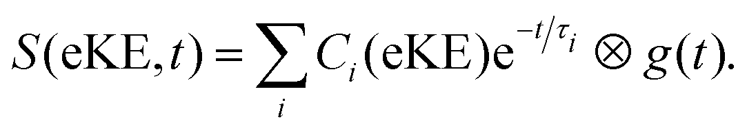
The photoinduced intramolecular dynamics of the prototypical aromatic molecule benzene have been the subject of many spectroscopic investigations. At low excess energies in the first excited singlet state, S₁(¹B_2u), the quantum yield for fluorescence (channel 1) is 0.2 and any non-radiative decay is slow and attributed to ISC (channel 2). When the excess energy reaches 3000 cm⁻¹, there is an abrupt loss of fluorescence accompanied by an increase in non-radiative decay. The origin of this sudden change in the photophysics, referred to as ‘channel 3’, was a source of debate since the original observation was first reported by Callomon and coworkers.²⁶ By using a combination of continuous molecular beam TRPES and quantum dynamics calculations,^25,27,28 we found that in addition to initial excited-state dynamics and ultrafast IC through a CI back to the ground state, ultrafast ISC occurred from the initially populated S₁(¹B_2u) state to an optically dark triplet state, challenging the traditional view that processes associated with a change in spin in simple organic hydrocarbons can be ignored in the first few picoseconds.

TRPES following photoexcitation to S₁ with 3070 cm⁻¹ of excess vibrational energy are presented in Fig. 5(a). The total integrated photoelectron signals as a function of pump–probe delay were fitted to biexponential functions (eqn (1)) and a plot of the ratio of the amplitude of the slow component to the amplitude of the fast component, as a function of probe wavelength was a step function centered at 250 nm (Fig. 5(b)), i.e. when the probe energy increases ≥4.96 eV, the observation window widens to cover more of the excited state potential energy surface. Such a distinct threshold is a signature of a new ionisation pathway opening up and provided the first hint that there must be a change in the electronic character along the adiabatic potential energy surface.

Fig. 5 (a) Contour plot of TRPES data following excitation of benzene with a 243 nm pump pulse and a 235 nm probe pulse as a function of pump–probe delay. Reproduced from J. Chem. Phys., 2012, 137, 204310, with the permission of AIP Publishing. (b) Plot of the ratio of the amplitudes of the slow and fast components of the biexponential decay of excited state population observed, following photoexcitation at 243 nm, plotted as a function of probe wavelength. Reproduced from ref. 25 with permission from Elsevier.

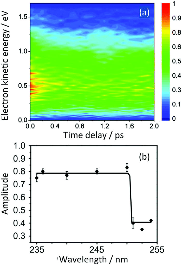
Simulations allowed us to distinguish between resonant and non-resonant (Fig. 3) contributions to the signal.²² Quantum dynamics calculations using potential surfaces calculated at the CASPT2 level with a (6,6) CAS and a Roos ANO basis set truncated to 6-31G* quality showed that the initial dynamics after excitation into S₁ is along the ‘prefulvene’ mode that takes benzene to the low lying S₁/S₀ CI. Importantly, as shown in Fig. 6(a), the S₁ and T₂ states are nearly degenerate over a wide range of geometries along this coordinate and, despite the very weak spin–orbit coupling, efficient ISC can take place, ending with population being trapped in T₁ (Fig. 6(b)).²⁸

Fig. 6 (a) Potential energy surfaces along the prefulvene mode (blue = S₀; red = T₁; black = T₂; green = S₁). (b) Excited state singlet (green) and singlet + triplet (red) populations as a function of time after vertical excitation into the S₁ state. The blue curve represents the approximate population in the Franck–Condon region. Adapted from ref. 27 with permission from the Royal Society of Chemistry.

4.2 Aniline

There has been considerable interest in the role of ¹πσ* states in the photochemistry of small aromatic molecules containing XH (X = O, N) groups.²⁹ These states are characterised by dissociative potential energy curves along the X–H stretching coordinate and have been shown to provide efficient electronic relaxation pathways to conical intersections with the electronic ground state and, consequently, play an important role in protecting biological molecules from harmful photochemical reactions.

Aniline is a structural motif found in the purine nucleotides, adenine and guanine and in the pyramidine nucleotide, cytosine. Numerous experimental studies of the photochemistry and photophysics of isolated aniline molecules in the gas-phase, using H-atom (Rydberg) photofragment translational spectroscopy,³¹ femtosecond pump–probe photoionisation spectroscopy³² and femtosecond pump–probe velocity map ion imaging,³³ have shed light on the N–H dissociation mechanism and timescales, but the mechanism of electronic relaxation remained a matter of debate until recently. By using a combination of continuous molecular beam TRPES measurements and detailed quantum chemistry investigations of the potential energy landscape and relaxation pathways, we found that following photoexcitation of the 2¹ππ* state, the dominant non-radiative decay pathway involved an extremely efficient method of transferring population straight back to the ground state.^30,34,35

The decay associated spectra derived from the TRPES (using eqn (2)) recorded following photoexcitation at 236 nm (5.25 eV) close to the 2¹ππ* ← S₀ absorption maximum revealed four time constants (Fig. 7). The spectrum associated with the 116 fs timescale was dominated by an intense, positive amplitude feature that corresponded energetically to the 2¹ππ* photoelectron spectrum. The spectrum associated with the 259 fs timescale had a positive amplitude in the region of the photoelectron spectrum, corresponding to the sharp π3s component of the 1¹π3s/πσ* state at 1.0 eV, and a negative amplitude corresponding to the photoelectron spectrum of the 1¹ππ* state, suggesting that population was flowing from the π3s component of the 1¹π3s/πσ* state to the 1¹ππ* state. The PAD of the sharp feature at 1.0 eV had β₂ = 0.8, consistent with ionisation from the atomic-like 3s character of the π3s component of the 1¹π3s/πσ* state (Section 2.4). The spectrum of the 81 ps component mirrored the shape of the negative amplitude component of the spectrum associated with the 259 fs decay.

Fig. 7 (a) Contour plot of TRPES data following excitation of aniline with a 236 nm pump pulse and a 300 nm probe pulse as a function of pump–probe delay. (b) Spectral components of the four decays derived using eqn (2). Adapted from ref. 30 with permission from the Royal Society of Chemistry.

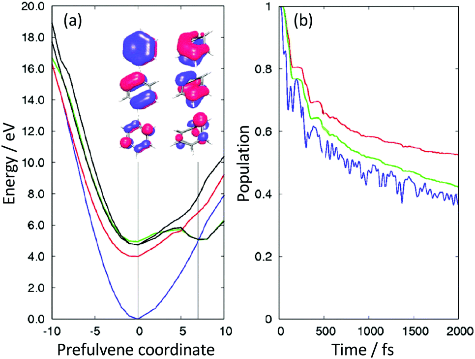
Detailed CASSCF and XMCQDPT2 (a variant of CASPT2) calculations were performed to explore the potential energy landscape and relaxation pathways of photoexcited aniline (Fig. 8).³⁵ The CASSCF calculations employed two different active spaces: an (8,7) CAS that included 3 occupied π orbitals, 3 unoccupied π* orbitals and the occupied N-atom lone pair orbital; a (10,9) CAS that also included the occupied 3s/πσ* orbital. These calculations found a new prefulvene-like minimum energy CI connecting the 1¹ππ* state with S₀ in which the carbon atom carrying the amino group is distorted out-of-plane. They showed us that excitation above the 1¹π3s/πσ* vertical excitation energy could be followed by relaxation from the 1¹ππ* state to S₀ through this CI. We also found a minimum energy CI connecting the 1¹π3s/πσ* and 1¹ππ* states close to the local minimum on the 1¹π3s/πσ* potential surface, suggesting that photoexcitation to the 1¹π3s/πσ* state could be followed by relaxation to the 1¹ππ* state, supporting our TRPES measurements. We also found evidence for a new pathway from the 2¹ππ* state to S₀ that we proposed to pass through a three-state CI involving the 2¹ππ*, 1¹π3s/πσ* and 1¹ππ* states. Subsequent TRPES measurements comparing the relaxation pathways of aniline and d₇-aniline at a range of photoexcitation wavelengths confirmed the existence of a three-state CI.³⁶ We have also developed a model of the coupled excited-state potential surfaces of aniline using EOM-CCSD/aug-cc-pVDZ calculations that reproduced the overlapping bands of the absorption spectrum and highlighted the significance of relaxation pathways due to coupling between bright valence and dark Rydberg states.³⁷ Other detailed TRPES measurements and calculations on aniline and its derivatives by Townsend and coworkers have investigated the nature of the evolution of the electronic character along the mixed Rydberg-valence 1¹π3s/πσ* surface.^38–40

Fig. 8 Schematic diagram illustrating key CASSCF and XMCQDPT2 calculated features on the potential energy landscape and relaxation pathways following photoexcitation to the first few singlet excited states of aniline. Reproduced from ref. 35 with permission from the Royal Society of Chemistry.

4.3 Pyrrole

Another example of a small aromatic molecule containing an N–H group is pyrrole, which is a common motif in many biologically important molecules, such as tryptophan, porphyrins, polyamide DNA binding agents and the phytochrome enzyme. It is also a basic building block in many technologically important systems, such as dye-sensitised solar cells and the polypyrrole conducting polymer. Consequently, its photochemistry and photophysics following excitation to the first band in its electronic absorption spectrum have attracted a great deal of interest.^15,41–43 We recently employed a combination of continuous molecular beam TRPES measurements and quantum dynamics calculations that revealed the relaxation mechanism following excitation of the second band in the electronic absorption spectrum.^44,45

The TRPES recorded following excitation at 200 nm (Fig. 9(a)) and decay associated spectra derived using eqn (2) (Fig. 9(b)), revealed a flow of population from electronic states producing photoelectrons with high eKE to electronic states producing photoelectrons with lower eKEs.⁴⁵ The electronic states producing photoelectrons with lower eKEs were then observed to decay out of the Franck–Condon window. Static and dynamic calculations were performed at the CASPT2/aug-cc-pVDZ level of theory with extra basis functions added to treat the Rydberg character of the low-lying excited states. An (8,8) CAS was used and the wavefunction state-averaged over seven states.⁴⁶

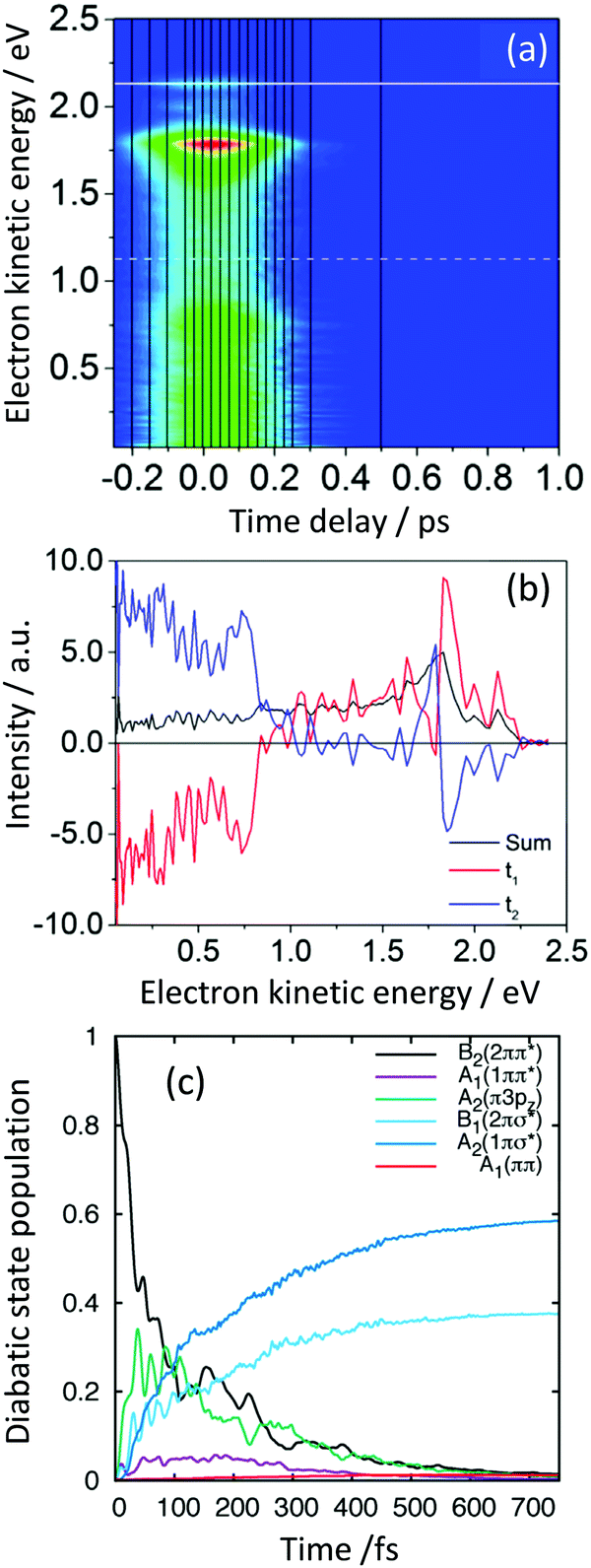Fig. 9 (a) Contour plot of TRPES data following excitation of pyrrole with a 200 nm pump pulse and a 300 nm probe pulse as a function of pump–probe delay. (b) Spectral components of the two decays derived using eqn (2) (red = 27 fs; blue = 34 fs). (c) Diabatic state populations calculated using wavepacket dynamics on a vibronic coupling model of the pyrrole excited-state manifold following excitation to the B₂(2¹ππ*) state. Reproduced from ref. 45 with permission from Elsevier.

The electronic states involved in the electronic relaxation processes were determined using conservation of energy and calculations of the Dyson norms for ionisation (Section 3.3) that showed B₂(2¹ππ*) and A₂(1¹πσ*) states ionised to the D₀ continuum and A₁(1¹ππ*) and B₁(2¹πσ*) states ionises to both the D₀ and D₁ continua. Thus, following photoexcitation of the B₁(2¹πσ*) state at 217 nm, the two measured time-constants, 13 fs and 29 fs, could be attributed to IC from the initially populated B₁(2¹πσ*) state to the A₂(1¹πσ*) state followed by population flow on the A₂(1¹πσ*) state out of the Franck–Condon region. Following photoexcitation of the B₂(2¹ππ*) state at 200 nm, the two measured time-constants, 27 fs and 34 fs, could be attributed to IC from the initially populated B₂(2¹ππ*) state to the B₁(2¹πσ*) and A₂(1¹πσ*) states.

Detailed quantum dynamics studies then allowed us to propose that following excitation of the B₂(2¹ππ*) state, population was transferred through the A₂(¹π3p_z) state to the B₁(2¹πσ*) state before being transferred to the A₂(1¹πσ*) state (Fig. 9(c)). Another recent study combining TRPES and quantum dynamics also found evidence for the involvement of the A₂(¹π3p_z) state in the electronic relaxation of pyrrole following photoexcitation at 200 nm.⁴⁷

4.4 Pyrrole dimer

Dimerisation of pyrrole has been found to open up additional relaxation pathways, such as a high-energy proton-coupled electron-transfer (ET) channel.^48,49 Using a combination of TRPES and quantum chemistry calculations, we found a new, low-energy, photoinduced ET mechanism in the pyrrole dimer.⁵⁰ We captured the electron transfer process, from the excited π-system of the donor pyrrole to a Rydberg orbital localised on the N-atom of the acceptor pyrrole, mediated by an N–H stretch on the acceptor molecule and found that the resulting charge-transfer state was surprisingly long-lived and led to efficient electronic relaxation.

The TRPES recorded following excitation at 245 nm (Fig. 10(a)) and decay associated spectra derived using eqn (2) (Fig. 10(b)), revealed dynamics occurring on two timescales of 46 fs and 270 fs. The 47 fs timescale had positive amplitudes in the range 0–1.3 eV but negative amplitudes around 1.45 eV, suggesting an evolution along the excited potential energy surface from a region with a photoelectron spectrum with lower eKE to a region with a photoelectron spectrum with higher eKE. The spectrum associated with the 270 fs timescale is centered around 1.45 eV with positive amplitude, suggesting that once populated, the region of the excited potential energy surface with a photoelectron spectrum with higher eKE decays out of the photoionisation window with a slightly longer timescale.

Fig. 10 (a) Contour plot of TRPES data following excitation of pyrrole dimers with a 245 nm pump pulse and a 300 nm probe pulse as a function of pump–probe delay. (b) Spectral components of the decays derived using eqn (2) (blue = 46 fs; green = 270 fs). (c) Adiabatic potential energy curves for the S₀ (black), S₁ (blue) and S₂ (red) states calculated at the DFT/MRCI/aug-cc-pVDZ level along the N–H dissociation coordinate of monomer A. This figure is taken from ref. 50.

The dimer is held together by an NH⋯π bond. CASPT2 calculations with an (8,8) CAS showed that the S₁ and S₂ states have 3s character at the Franck–Condon point. The S₁(π_B3s_A) state has charge-transfer character, with the dominant configuration corresponding to excitation from a π orbital localised on monomer B to the 3s orbital localised on the N-atom of monomer A (Fig. 10(c)). In contrast, the S₂(π_A3s_A) state is dominated by a configuration corresponding to excitation from a π orbital localised on monomer A to the 3s orbital localised on the same monomer, reminiscent of the A₂(π3s) state of the pyrrole monomer. EOM-IP-CCSD/aug-cc-pVDZ photoionisation cross-section calculations revealed that the S₁ state ionises preferentially to the D₀ state but the S₂ state ionises preferentially to the higher lying D₂ state. From the calculated VEEs, IEs and photoionisation cross-sections, we were able to deduce that following photoexcitation of the S₂ state at 245 nm, population was flowing to the S₁ charge-transfer state on a timescale of 46 fs and that this charge transfer state then decayed on a slightly longer timescale of 270 fs. Calculated potential energy surfaces of the S₀, S₁ and S₂ states along the N–H dissociation coordinate r of monomer A are presented in Fig. 10(c) and show that the transfer in population from the S₂ state to the S₁ state is likely to occur at the avoided crossing along the N–H bond stretch. Similar time-signatures were subsequently observed in a pump–probe ionisation study of size-selected pyrrole dimers.⁵¹

4.5 Green fluorescent protein chromophore anion

Green fluorescent protein (GFP) is the most widely used fluorescent protein for in vivo monitoring of biological and biochemical processes. The chromophore that lies at the heart of GFP is 4-hydroxybenzylidene-1,2-dimethylimidazolinone, p-HBDI. Excitation of GFP results in strong fluorescence (Φ ∼ 0.8) from the deprotonated anionic form of the chromophore, p-HBDI⁻. The fluorescence is lost when the protein is denatured, although it returns upon renaturation and isolated p-HBDI⁻ is virtually non-fluorescent in solution. Interestingly, p-HBDI⁻in vacuo has an electronic absorption spectrum that is similar to that of the native protein in its anionic form but it is non-fluorescent at room temperature.

By using a combination of ESI (Section 2.2), TRPES measurements and quantum chemistry calculations we were able to unravel the excited state dynamics of p-HBDI⁻in vacuo.⁵² The decay associated spectra derived from the TRPES using eqn (2) (Fig. 11) revealed a flow of population from electronic states producing photoelectrons with high eKE to electronic states producing photoelectrons with lower eKEs on a timescale of 330 fs. The electronic states producing photoelectrons with lower eKEs were then observed to decay out of the Franck–Condon window on a timescale of 1.4 ps.

Fig. 11 (a) TRPES following excitation of pHBDI⁻ with a 500 nm pump pulse and an 800 nm probe pulse as a function of pump–probe delay. (b) Spectral components of the two decays derived using eqn (2) (green = 330 fs; blue = 1.4 ps; sum = blue). (c) Schematic potential energy curves of S₁ and D₀ along the minimum energy path from the Franck–Condon (FC) region to the fluorescent state (FS) and twisted intermediate (TI) together with CASPT2 calculated energies in eV. Adapted from ref. 52 with permission from the Royal Society of Chemistry.

CASSCF calculations of the energies of key geometries on the excited S₁ potential energy surface of the anion and the D₀ potential energy surface of the corresponding neutral radical were performed using a (12,11) CAS and a 6-31G* basis set and these were improved using the CASPT2 method with an ANO-pVDZ basis set. These calculations (Fig. 11(c)) allowed us to assign the 330 fs timescale to rotation about the bridging C–C bond to form a twisted intermediate and the 1.4 ps timescale to dynamics away from the twisted intermediate towards a CI with the ground state. Remarkably, these results were very similar to measurements of timescales for the non-radiative decay of p-HBDI⁻ in solution,⁵³ pointing to a large influence of the protein environment on the excited S₁ potential energy surface. Subsequent TRPES measurements by Verlet and coworkers found a faster timescale of 40 fs following excitation at higher photon energies.⁵⁴ Recent time-resolved action spectroscopy measurements and XMCQDPT2 calculations by Andersen and Bochenkova and coworkers have shown that when the anions are cooled to 100 K, population is trapped on the S₁ potential energy surface for 1.2 ns, which is long enough for fluorescence to compete with IC.⁵⁵

5 Conclusion

TRPES is an ideal tool for following the time-evolution of photoexcited molecules, which are particularly complicated because many reaction pathways are often accessible. To maximise the information that can be extracted from TRPES measurements requires calculations that provide details of accessible states and available pathways. The interplay between experiment and theory is key, with each one validating the other. The examples described in this review illustrate the mechanistic information that can be obtained: ISC in benzene, photodissociation in aniline and pyrrole, charge-transfer in the pyrrole dimer and fluorescence quenching in the green fluorescent protein chromophore. We are now in a position where experimental and computational techniques can be applied in a fairly routine manner to a wide range of reasonably complex systems and the information that is emerging is allowing us to build up a detailed picture of how a wide range of molecules respond to light; however, there are still major experimental and computational challenges. These include developing TRPES methodology for chromophores in realistic environments, combining accurate potential energy surfaces with accurate nuclear dynamics and calculating time-resolved photoelectron spectra. We are not yet at the stage of having a set of ‘rules’ for photochemistry, like the Polanyi rules that guide our thinking about how molecular vibrations control the pathway through a transition-state on the ground-electronic state, and the results are often system-dependent and sometimes surprising. The next few years will undoubtedly see an increase in the information available and further improvements in the experimental and theoretical techniques employed in this flourishing area of research and perhaps the emergence of a set of rules for excited-state chemistry.

Conflicts of interest

There are no conflicts to declare.

Acknowledgements

We acknowledge the EPSRC for supporting this work and thank our co-workers and collaborators for their contributions to the work described in this review.

References

1. M. A. Robb, Conical Intersections: Theory, Computation and Experiment, 2011, pp. 3–50.
2. A. Stolow and J. G. Underwood, Adv. Chem. Phys., 2008, 139, 497–583.
3. T. Suzuki, Int. Rev. Phys. Chem., 2012, 31, 265–318.
4. R. Spesyvtsev, J. G. Underwood and H. H. Fielding, Ultrafast Phenomena in Molecular Sciences: Femtosecond Physics and Chemistry, 2014, pp. 99–117.
5. K. L. Reid, Annu. Rev. Phys. Chem., 2003, 54, 397–424.
6. R. Seidel, B. Winter and S. E. Bradforth, Annu. Rev. Phys. Chem., 2016, 67, 283–305.
7. Conical intersections: electronic structure, dynamics and spectroscopy, ed. W. Domcke, D. R. Yarkony and H. Köppel, World Scientific, Singapore, 2004.
8. G. A. Worth and L. S. Cederbaum, Annu. Rev. Phys. Chem., 2004, 55, 127–158.
9. M. J. G. Peach, P. Benfield, T. Helgaker and D. J. Tozer, J. Chem. Phys., 2008, 128, 044118.
10. M. Beck, A. Jäckle, G. Worth and H.-D. Meyer, Phys. Rep., 2000, 324, 1–106.
11. A. W. Jasper, S. Nangia, C. Zhu and D. G. Truhlar, Acc. Chem. Res., 2006, 39, 101–108.
12. L. Wang, A. Akimov and O. V. Prezhdo, J. Phys. Chem. Lett., 2016, 7, 2100–2112.
13. G. W. Richings, I. Polyak, K. E. Spinlove, G. A. Worth, I. Burghardt and B. Lasorne, Int. Rev. Phys. Chem., 2015, 34, 269–308.
14. G. A. Worth and M. A. Robb, Adv. Chem. Phys., 2002, 124, 355–432.
15. M. Barbatti, M. Vazdar, A. J. Aquino, M. Eckert-Maksić and H. Lischka, J. Chem. Phys., 2006, 125, 164323.
16. M. Richter, P. Marquetand, J. González-Vázquez, I. Sola and L. González, J. Chem. Theory Comput., 2011, 7, 1253–1258.
17. B. F. E. Curchod, U. Rothlisberger and I. Tavernelli, ChemPhysChem, 2013, 14, 1314–1340.
18. K. Saita and D. V. Shalashilin, J. Chem. Phys., 2012, 137, 22A506.
19. M. Ben-Nun and T. J. Martínez, Adv. Chem. Phys., 2002, 121, 439–512.
20. C. M. Oana and A. I. Krylov, J. Chem. Phys., 2007, 127, 234106.
21. L. S. Cederbaum, W. Domcke, J. Schirmer and W. Von Niessen, Adv. Chem. Phys., 1986, 65, 115–159.
22. G. A. Worth, R. E. Carley and H. H. Fielding, Chem. Phys., 2007, 338, 220–227.
23. G. W. Richings and G. A. Worth, J. Chem. Phys., 2014, 141, 244115.
24. H. R. Hudock, B. G. Levine, A. L. Thompson, H. Satzger, D. Townsend, N. Gador, S. Ullrich, A. Stolow and T. J. Martínez, J. Phys. Chem. A, 2007, 111, 8500–8508.
25. D. S. N. Parker, R. S. Minns, T. J. Penfold, G. A. Worth and H. H. Fielding, Chem. Phys. Lett., 2009, 469, 43–47.
26. J. H. Callomon, T. M. Dunn and I. M. Mills, Philos. Trans. R. Soc., A, 1966, 259, 499–532.
27. R. S. Minns, D. S. N. Parker, T. J. Penfold, G. A. Worth and H. H. Fielding, Phys. Chem. Chem. Phys., 2010, 12, 15607–15615.
28. T. J. Penfold, R. Spesyvtsev, O. M. Kirkby, R. S. Minns, D. S. N. Parker, H. H. Fielding and G. A. Worth, J. Chem. Phys., 2012, 137, 204310.
29. M. N. R. Ashfold, G. A. King, D. Murdock, M. G. D. Nix, T. A. A. Oliver and A. G. Sage, Phys. Chem. Chem. Phys., 2010, 12, 1218–1238.
30. R. Spesyvtsev, O. M. Kirkby, M. Vacher and H. H. Fielding, Phys. Chem. Chem. Phys., 2012, 14, 9942–9947.
31. G. A. King, T. A. A. Oliver and M. N. R. Ashfold, J. Chem. Phys., 2010, 132, 214307.
32. R. Montero, A. P. Conde, V. Ovejas, R. Martínez, F. Castaño and A. Longarte, J. Chem. Phys., 2011, 135, 054308.
33. G. M. Roberts, C. a. Williams, J. D. Young, S. Ullrich, M. J. Paterson and V. G. Stavros, J. Am. Chem. Soc., 2012, 134, 12578–12589.
34. R. Spesyvtsev, O. M. Kirkby and H. H. Fielding, Faraday Discuss., 2012, 157, 165–179.
35. M. Sala, O. M. Kirkby, S. Guérin and H. H. Fielding, Phys. Chem. Chem. Phys., 2014, 16, 3122–3133.
36. O. M. Kirkby, M. Sala, G. Balerdi, R. de Nalda, L. Bañares, S. Guérin and H. H. Fielding, Phys. Chem. Chem. Phys., 2015, 17, 16270–16276.
37. F. Wang, S. Neville, R. S. Wang and G. A. Worth, J. Phys. Chem. A, 2013, 117, 7298–7307.
38. J. O. F. Thompson, R. a. Livingstone and D. Townsend, J. Chem. Phys., 2013, 139, 034316.
39. J. O. F. Thompson, L. Saalbach, S. W. Crane, M. J. Paterson and D. Townsend, J. Chem. Phys., 2015, 142, 114309.
40. M. M. Zawadzki, M. Candelaresi, L. Saalbach, S. W. Crane, M. J. Paterson and D. Townsend, Faraday Discuss., 2016, 194, 185.
41. B. Cronin, A. L. Devine, M. G. D. Nix and M. N. R. Ashfold, Phys. Chem. Chem. Phys., 2006, 8, 3440–3445.
42. R. Montero, Á. P. Conde, V. Ovejas, M. Fernández-Fernández, F. Castaño, R. Javier, J. R. Vázquez de Aldana, A. Longarte, R. Montero, Á. P. Conde, V. Ovejas, M. Fernández-Fernández, F. Castaño, J. R. V. D. Aldana and A. Longarte, J. Chem. Phys., 2012, 2012, 064317.
43. G. M. Roberts, C. A. Williams, H. Yu, A. S. Chatterley, J. D. Young and V. G. Stavros, Faraday Discuss., 2013, 163, 95–116.
44. G. Wu, S. P. Neville, O. Schalk, T. Sekikawa, M. N. R. Ashfold, G. A. Worth, G. Wu, S. P. Neville, O. Schalk, T. Sekikawa, A. Stolow, G. Wu, S. P. Neville, O. Schalk and T. Sekikawa, J. Chem. Phys., 2015, 142, 074302.
45. O. M. Kirkby, M. A. Parkes, S. P. Neville, G. A. Worth and H. H. Fielding, Chem. Phys. Lett., 2017, 683, 179–185.
46. S. P. Neville and G. A. Worth, J. Chem. Phys., 2014, 140, 34317.
47. T. Geng, O. Schalk, S. P. Neville, T. Hansson and R. D. Thomas, J. Chem. Phys., 2017, 146, 144307.
48. V. Poterya, V. Profant, M. Fárník, P. Slavíček and U. Buck, J. Chem. Phys., 2007, 127, 064307.
49. P. Slavíček and M. Fárník, Phys. Chem. Chem. Phys., 2011, 13, 12123–12137.
50. S. P. Neville, O. M. Kirkby, N. Kaltsoyannis, G. A. Worth and H. H. Fielding, Nat. Commun., 2016, 7, 11357.
51. R. Montero, I. Leon, J. A. Fernandez and A. Longarte, J. Phys. Chem. Lett., 2016, 7, 2797–2802.
52. C. R. S. Mooney, D. A. Horke, A. S. Chatterley, A. Simperler, H. H. Fielding and J. R. R. Verlet, Chem. Sci., 2013, 4, 921–927.
53. D. Mandal, T. Tahara and S. R. Meech, J. Phys. Chem. B, 2004, 108, 1102–1108.
54. C. W. West, J. N. Bull, A. S. Hudson, S. L. Cobb and J. R. R. Verlet, J. Phys. Chem. B, 2015, 119, 3982–3987.
55. A. Svendsen, H. V. Kiefer, H. B. Pedersen, A. V. Bochenkova and L. H. Andersen, J. Am. Chem. Soc., 2017, 139, 8766–8771.

---