
 Open Access Article
 This Open Access Article is licensed under a Creative Commons Attribution-Non Commercial 3.0 Unported Licence
Model – free approach to quadrupole spin relaxation in solid 209Bi-aryl compounds
Danuta
Kruk
 *a,
Christian
Goesweiner
b,
Elzbieta
Masiewicz
a,
Evrim
Umut
a,
Carina
Sampl
c and
Hermann
Scharfetter
b
*a,
Christian
Goesweiner
b,
Elzbieta
Masiewicz
a,
Evrim
Umut
a,
Carina
Sampl
c and
Hermann
Scharfetter
b
aUniversity of Warmia & Mazury in Olsztyn, Faculty of Mathematics and Computer Science, Słoneczna 54, PL-10710 Olsztyn, Poland. E-mail: danuta.kruk@matman.uwm.edu.pl; Tel: +48 89 524 60 11
bInstitute of Medical Engineering, Graz University of Technology, Stremayrgasse 16/III, A-8010 Graz, Austria
cInstitute of Inorganic Chemistry, Graz University of Technology, Stremayrgasse 9, 8010 Graz, Austria
First published on 4th September 2018
Abstract
Nuclear Quadrupole Resonance (NQR) experiments were performed for deuterated and non-deuterated triphenylbismuth (BiPh3) to inquire into 209Bi relaxation mechanisms. The studies are motivated by the idea of exploiting Quadrupole Relaxation Enhancement (QRE) as a novel contrast mechanism for Magnetic Resonance Imaging. From this perspective relaxation features of nuclei possessing quadrupole moment (quadrupole nuclei) are of primary importance for the contrast effect. Spin–spin relaxation rates associated with the NQR lines were described in terms of the Redfield relaxation theory assuming that the relaxation is caused by fluctuations of the electric field gradient tensor at the position of the quadrupole nucleus that are described by an exponential correlation function. The description referred to as a model-free approach is an analogy of the description used for paramagnetic contrast agents. It was demonstrated that for the deuterated compound this approach captures the essential features of 209Bi relaxation, but it should not be applied for non-deuterated compounds as dipolar interactions between neighbouring protons and the quadrupole nucleus considerably contribute to the relaxation of the last one. Thus, the relaxation scenario for species containing quadrupole nuclei is fundamentally different than for paramagnetic contrast agents and this fact has to be taken into account when predicting contrast effects based on QRE.
1. Introduction
Contrast agents in Magnetic Resonance Imaging (MRI) are used to increase the difference between spin relaxation of water protons in healthy and pathological tissue. The difference can be increased due to Paramagnetic Relaxation Enhancement (PRE) effects caused by paramagnetic contrast agents (for instance complexes of transition and rare earth ions, like Gd3+).1–5 Strong magnetic electron–proton dipole–dipole interactions between the electron spin of the paramagnetic species and spins of water protons lead to very fast proton spin relaxation (the relaxation rates become larger – in other words, the relaxation is enhanced). Taking into account that the 1H relaxation rate depends on a square of the electron gyromagnetic factor (being by a factor of about 659 larger than the proton gyromagnetic factor) one could expect a very large enhancement of the 1H relaxation rate. However, the observed relaxation enhancement is much smaller as a result of fast electron spin relaxation caused by Zero Field Splitting (ZFS) interaction.6–11 For not immobilized small paramagnetic complexes the limiting factor is their fast molecular tumbling, especially at high fields.To some extent one can consider the Quadrupole Relaxation Enhancement (QRE)12–20 as a counterpart of PRE. Yet the similarity concerns only the analogy in the Hamiltonian forms of ZFS and quadrupole interactions; the physical backgrounds of QRE and PRE are different. When the electron spin (a paramagnetic complex) is replaced by a species containing high spin quantum number (S ≥ 1) nucleus (referred to as a quadrupole nucleus), the quadrupole nucleus and neighbouring protons become coupled by dipole–dipole interactions (analogously to the electron–proton coupling for PRE) being the source of 1H relaxation. At the same time the energy level structure of the quadrupole nucleus is determined by a superposition of its quadrupole and Zeeman couplings. As the quadrupole coupling is independent of the magnetic field, there are magnetic fields (1H resonance frequencies) at which the 1H energy level splitting matches one of the transitions of the quadrupole nucleus between its energy levels. When the dynamics of the system is slow at these magnetic fields the 1H magnetization can be transferred to the quadrupole nucleus; this manifests itself as a faster decay of the 1H magnetization – i.e. a frequency specific 1H spin–lattice relaxation enhancement. As QRE effects manifest themselves only at selected frequencies (in contrary to the PRE observed in the whole frequency range), they can be switched on and off in response to subtle changes of the electric field gradient in the tissue – this gives rise to the question whether QRE effects can be exploited as a novel, smart MRI contrast mechanism.
The PRE effect has been a subject of extensive theoretical studies due to its medical relevance posing, at the same time, a very interesting problem of quantum-mechanical theory of spin relaxation.6–11,21–31 The most demanding part of the theoretical description is the electron spin relaxation. The theory of PRE has started from a very simple description of the electron spin relaxation, just introducing for this purpose two parameters: electron spin–lattice and spin–spin relaxation rates.27 At this stage there was no question about the specific electron spin relaxation mechanism. This approach has turned out to be insufficient; in this way one cannot satisfactorily explain the 1H relaxation enhancement monitored versus the magnetic field (i.e.1H resonance frequency). The oversimplification of this approach has two reasons: the electron spin relaxation is treated as independent of the magnetic field (this is incorrect) and multi-exponentiality of the relaxation (present for high electron spin quantum numbers) is not taken into account. In the next step, a more appropriate description of the electron spin relaxation based on the Redfield relaxation theory has been developed.8,11,22,28,29 Such an approach requires a well-defined model of the relaxation process. This has given rise to the so called pseudorotational model,7–11,25,26,29 that can be referred to as a model-free approach. According to this approach the fluctuations of the ZFS interaction, being the source of the electron spin relaxation, have a constant (time independent) amplitude and are characterized by an exponential correlation function. The great advantages of this approach are its mathematical simplicity and the number of parameters (only two: the amplitude of the fluctuating part of the ZFS interaction and the characteristic time constant of the fluctuations referred to as a correlation time). This concept has turned out to be a success – it has led to very good agreement of the theoretically predicted PRE effect with experimental data for numerous paramagnetic contrast agents. Thus its accuracy has not been much questioned. A rare example of a verification of the model-free approach is the attempt to interpret Electron Spin Resonance lineshape and PRE effects for some Gd3+ complexes in terms of the same electron spin parameters.31 The output can be a matter of debate – the agreement with both kinds of experimental data is moderate. One should keep in mind that for PRE effects one can talk about a hierarchy of events: the electron spin relaxation is independent of the presence of neighbouring protons (the fluctuating part of the ZFS interaction provides the predominating mechanism of the electron spin relaxation), while it contributes to the fluctuation of the electron–proton dipole–dipole interaction being the source of the 1H relaxation and hence affects the PRE effect.
To explore the possibility of using QRE effects as a contrast mechanism it is necessary to understand the relaxation properties of the quadrupole nucleus and formulate a proper relaxation model. Among several high spin quadrupole nuclei we consider 209Bi as a very promising candidate because of its large quadrupole moment that gives the opportunity to observe QRE effects at high magnetic field (3T) used in clinical MRI scanners and because of its expected lower toxicity compared to gadolinium.
Nuclear Quadrupole Resonance (NQR) spectroscopy gives access to the spin–spin relaxation. In NQR experiments one can detect several lines corresponding to single-quantum transition frequencies between energy levels of the quadrupole nucleus (4 for the spin quantum number of 209Bi, S = 9/2) and measure the associated spin–spin relaxation rates. This paper is meant to reveal to which extent relaxation properties of a quadrupole nucleus in solids can be captured by a description of fluctuating quadrupole interactions analogous to the model-free approach formulated for the ZFS in the case of high electron spin species.
Besides the context of medical applications, plausibility of this approach would give access to internal dynamics of solids containing quadrupole nuclei by means of NQR spectroscopy – one would be able reliable estimate the timescale of dynamical processes. One could argue at this stage that relaxation mechanisms for solids can hardly be transferred to the case of solutions. One should, however, take into account that to be used as MRI contrast agents the molecules containing quadrupole nuclei will be embedded in a matrix forming nanoparticles to ensure slow rotation of the whole species. Thus the quadrupole relaxation will result from internal dynamics of a network of the molecules similarly to solids.
Quadrupole relaxation in solids is commonly attributed to phonon dynamics. Relaxation models assuming Raman phonon dynamics have been discussed in the literature for different compounds.32–39 Such models include many parameters and, even though, quite often do not lead to good agreement with the experiment. Actually, for the same reasons phonon models of electron spin relaxation for paramagnetic complexes has not gained much popularity.
The paper is organized as follows: in Section 2 the principles of quadrupole relaxation are presented, Section 3 contains experimental details, in Section 4 NQR data for 209Bi containing solids (deuterated- and non-triphenylbismuth (BiPh3)) are presented and discussed, while Section 5 includes concluding remarks.
2. Quadrupole relaxation
Nuclei of spin quantum numbers S ≥ 1 exhibit quadrupole interaction when placed in an electric field gradient. The quadrupole Hamiltonian is given in the principal axis system of the electric field gradient as:40–42 | (1) |
 ,
,  and
and  . For S = 9/2(209Bi) and η = 0 this leads to the following energy levels corresponding to the magnetic quantum numbers, mS, determining the set of eigenvectors of the quadrupole coupling, {|S,mS〉}:
  ,
,  ,
,  ,
,  and
and  . Thus, in NQR experiments one can observe four transitions at the frequencies of:
  ,
,  ,
,  and
and 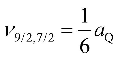 , where νmS,mS′ = νmS − νmS′ = να − νβ = ναβ denotes differences between energy levels corresponding to different magnetic spin quantum numbers. To obtain the energy level structure and hence the transition frequencies for η ≠ 0 the Hamiltonian of eqn (1) has to be represented in the {|i〉 = |S,mS〉} basis (the matrix is not diagonal) and diagonalized. The matrix representation is given in Appendix. As a result of the diagonalization one obtains a set of eigenvalues (energy levels) {Eα} associated with the corresponding eigenvectors {ψα} given as linear combinations of the {|i〉 = |S,mS〉} vectors:
  .
.
The NQR lines are associated with spin–spin relaxation rates. To discuss this subject, in the first step, one has to determine the relaxation mechanism. As anticipated in Introduction, our goal is to explore to which extend the relaxation properties can be explained by a very simple model assuming that the relaxation is caused by local fluctuations of the quadrupole interaction characterized by an amplitude ΔaQ and a correlation time τQ (a characteristic time constant describing the time scale of the fluctuations). Moreover, the model assumes that the amplitude is time independent so the stochastic fluctuations concern the orientation of the temporary direction of the principal axis system of the electric field gradient tensor with respect to its averaged orientation. The relative orientation of these two frames is described by an angle Ω(t); its fluctuations are described by an exponential correlation function. This concept leads to the following form of the perturbing (leading to the relaxation process) Hamiltonian HQ′(t):
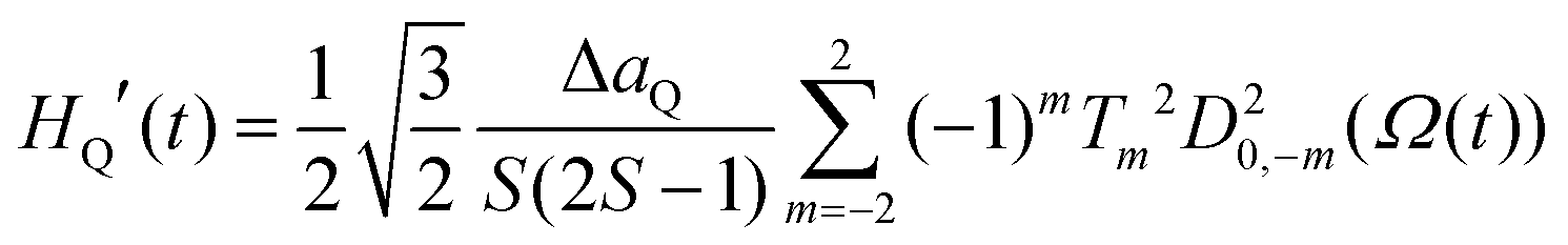 | (2) |
 | (3a) |
 | (3b) |
 | (3c) |
 | (3d) |
 .40–44 In the extreme narrowing case (for very short τQ, when ωτQ ≪ 1) the relaxation rates converge to:
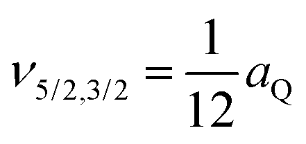
  ,
,  ,
,  and
and  .
.
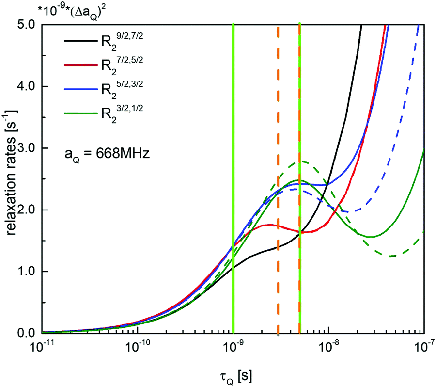
Before proceeding to the data analysis it is worth to compare the predictions of eqn (3a)–(3d) with the general expression derived in Appendix. Anticipating the experimental data, in Fig. 1 ratios between the relaxation rates R3/2,1/22, R5/2,3/22, R7/2,5/22, R9/2,7/22 for aQ = 668 MHz, η = 0 and their corresponding counterparts for aQ = 668 MHz, η = 0.1 are plotted versus the correlation time τQ. One can conclude from this comparison that for aQ and η values being close to the selected ones, one can use eqn (3a)–(3d) as a good approximation only for R7/2,5/22 and R9/2,7/22.
 | ||
| Fig. 1 The ratios between the relaxation rates R3/2,1/22, R5/2,3/22, R7/2,5/22, R9/2,7/22 for η = 0 and η = 0.1 with aQ = 668 MHz, are plotted versus the correlation time τQ. | ||
Eventually, one should stress that for η ≠ 0 one cannot talk about relaxation rates  as the vectors {|i〉 = |S,mS〉} are not eigenvectors of the system anymore. In the forthcoming sections we use this notation only as an approximation because the relaxation rates for η = 0 and η = 0.1 do not differ much for the range of the correlation time τQ which will turn out to be relevant for the analysis (see Section 4).
3. Experimental details
209Bi NQR experiments were performed for deuterated and non-deuterated triphenylbismuth (BiPh3) at 310 K, 300 K and 77 K. Structure of the non-deuterated compound is shown in Fig. 2. | ||
| Fig. 2 Structure of non-deuterated triphenylbismuth (BiPh3). | ||
The experimental data were acquired with the commercially available “Scout” (Tecmag, Inc., USA) pulse-type NQR-spectrometer using a two sets of shielded RF transmit/receive coils. One set of probe coils covers a frequency range of 20 MHz to 130 MHz (for 77 K and RT (300 K)) and another set of coils covers a range of 55 MHz to 160 MHz (for temperatures between 283 K to 323 K). In consequence, experiments at 310 K were limited to the three higher transition frequencies.
The coils are driven by a 500 W power amplifier. The solid, crystalline powder samples were encapsulated in glass vials of 10 mm diameter. For the measurements at RT and 310 K temperature stability was maintained by a flow of dry air controlled by a feedback unit using a type K thermocouple placed in the sample vial. Some of the coils were self-built45 featuring a special low-temperature front-end46 for diving them directly into liquid nitrogen. Temperature accuracy was 0.5 K for measurements at 300 K and 310 K respectively. For measuring spin–spin relaxation rates, R2, a standard spin echo sequence with variable echo time was used. The spin-echo maxima versus time were fitted using a mono-exponential model for the decay of the signal amplitude.
4. Experimental data and analysis
We begin the analysis of 209Bi spin–spin relaxation data with deuterated BiPh3 (310 K) as in this case the relaxation solely originates from fluctuations of the electric field gradient tensor at the position of 209Bi (i.e. the fluctuating part of the quadrupole interaction, HQ′(t)). Table 1 includes three experimental transition frequencies obtained for this compound. The transitions are numbered according to their increasing frequency. As already explained in Section 3, above room temperature we do not have experimental opportunities to perform the NQR experiment at frequencies corresponding to the lowest transition frequency of about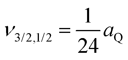 (it depends on η). Comparing these values with the energy levels (and hence transition frequencies) obtained by diagonalizing the matrix representation of the Hamiltonian HQ for η ≠ 0 (given in Appendix), the quadrupole parameters aQ = 668.83 MHz and η = 0.087 have been determined. For these parameters the theoretical transition frequencies agree very well with the experimental ones. As far as relaxation is concerned, the first observation which should be made is that the relaxation rates decrease with increasing frequency: R5/2,3/22 > R7/2,5/22 > R9/2,7/22. As we are aware that the discussed model is a simplification, in the first step one should figure out whether such a dependence can be reproduced. For this purpose in Fig. 3 the relaxation rates R3/2,1/22, R5/2,3/22, R7/2,5/22 and R9/2,7/22 are plotted versus the correlation time τQ (aQ = 668 MHz, η = 0 and η = 0.1). One can see from Fig. 3 that the appropriate order of the relaxation rates (R5/2,3/22 > R7/2,5/22 > R9/2,7/22) can be obtained for τQ in the range of 1.0 × 10⁻⁹–5.0 × 10⁻⁹ s (solid vertical lines in Fig. 3). The “best” τQ value has been obtained by minimizing the value of
  . The summation goes over all relaxation rates, Ri2,exp denotes the i-th experimental value, while Ri2,theory is the corresponding theoretical value; Δ does not depend of ΔaQ. The theoretical relaxation rates have been calculated from the general expressions, presented in Appendix, for η ≠ 0. Applying this strategy τQ = 1.58 × 10⁻⁹ s has been obtained; the appropriate values of the relaxation rates can be reached for ΔaQ = 0.98 MHz. The values of Ri2,theory obtained for these parameters are included in Table 1. One can see that the frequency dependence of the theoretical relaxation rates is stronger than of the experimental ones. Nevertheless, one can say that the model captures essential features of the quadrupole relaxation; Table 1 also includes the discrepancies (in %) between the experimental and theoretical values of the relaxation rates. For comparison, corresponding values obtained for η = 0 from eqn (3a)–(3d) are also shown in Table 1.
![[thin space (1/6-em)]](https://www.rsc.org/images/entities/char_2009.gif) )”, denote theoretical relaxation rates for η = 0 (ΔaQ and τQ remain unchanged), “TFs” denotes NQR transition frequencies
)”, denote theoretical relaxation rates for η = 0 (ΔaQ and τQ remain unchanged), “TFs” denotes NQR transition frequencies
| Transition number | Experimental TFs [MHz] | Theoretical TFs [MHz] | Experimental relaxation rates [s−1] | Theoretical relaxation rates [s−1] | Deviation [%] |
|---|---|---|---|---|---|
| BiPh3 – deuterated; aQ = 668.83 MHz, η = 0.087, ΔaQ = 0.98 MHz, τQ = 1.58 × 10⁻⁹ s, T = 310 K | |||||
| 2 | 55.20 | 55.21 | 1600 | 1757(1770) | 8.9 |
| 3 | 83.49 | 83.49 | 1590 | 1611(1611) | 1.3 |
| 4 | 111.40 | 111.40 | 1404 | 1204(1203) | 16.6 |
| BiPh3 – deuterated; aQ = 669.87 MHz, η = 0.098, ΔaQ = 0.98 MHz, τQ = 3.63 × 10⁻⁹ s, T = 300 K | |||||
| 1 | 29.82 | 30.22 | 2392 | 2709(2552) | 11.7 |
| 2 | 55.25 | 55.16 | 1905 | 2185(2225) | 12.8 |
| 3 | 83.58 | 83.58 | 1572 | 1629(1622) | 3.5 |
| 4 | 111.56 | 111.56 | 1565 | 1394(1392) | 12.3 |
| BiPh3 – deuterated; aQ = 685.63 MHz, η = 0.095, ΔaQ = 0.41 MHz, τQ = 4.32 × 10⁻⁹ s, T = 77 K | |||||
| 1 | 30.72 | 30.80 | 1613 | 413(453) | 290.8 |
| 2 | 56.52 | 56.50 | 509 | 400(383) | 27.2 |
| 3 | 85.56 | 85.56 | 232 | 273(271) | 14.9 |
| 4 | 114.19 | 114.19 | 215 | 253(252) | 15.0 |
| BiPh3; aQ = 668.32 MHz, η = 0.087, ΔaQ = 1.25 MHz, τQ = 3.71 × 10⁻⁹ s, T = 310 K | |||||
| 2 | 55.14 | 55.16 | 3610 | 3577(3632) | 0.9 |
| 3 | 83.42 | 83.42 | 2294 | 2637(2638) | 13.0 |
| 4 | 111.32 | 111.32 | 2058 | 2283(2281) | 9.8 |
| BiPh3; aQ = 668.87 MHz, η = 0.083, ΔaQ = 1.25 MHz, τQ = 4.03 × 10⁻⁹ s, T = 300 K | |||||
| 1 | 29.76 | 29.55 | 12500 |
4471(4253) | 179.6 |
| 2 | 55.21 | 55.26 | 4505 | 3589(3643) | 25.5 |
| 3 | 83.50 | 83.50 | 2525 | 2618(2608) | 3.6 |
| 4 | 111.42 | 111.42 | 2304 | 2334(2331) | 1.3 |
| BiPh3; aQ = 684.63 MHz, η = 0.090, ΔaQ = 0.95 MHz, τQ = 4.45 × 10⁻⁹ s, T = 77 K | |||||
| 1 | 30.64 | 30.53 | 9803 | 2677(2442) | 266.3 |
| 2 | 56.45 | 56.48 | 2538 | 2016(2055) | 25.9 |
| 3 | 85.45 | 85.45 | 1247 | 1467(1452) | 15.0 |
| 4 | 114.03 | 114.03 | 1217 | 1373(1370) | 11.3 |
 | ||
| Fig. 3 The relaxation rates R3/2,1/22, R5/2,3/22, R7/2,5/22 and R9/2,7/22 plotted versus the correlation time τQ in case when η = 0 (dashed line) and η = 0.1 (solid line) for aQ = 668 MHz. Solid vertical lines show the time range in which the relationship R5/2,3/22 > R7/2,5/22 > R9/2,7/22 is fulfilled, dashed vertical lines correspond to the range in which the relationship R3/2,1/22 > R5/2,3/22 > R7/2,5/22 > R9/2,7/22 holds. | ||
For the lower temperature (300 K) four NQR lines (including the lowest transition frequency) have been measured. The frequencies of the individual lines are given in Table 1. They correspond to aQ = 669.87 MHz and η = 0.098; the parameters slightly differ from those for 310 K. The previous order of the relaxation rate is now extended to the relationship: R3/2,1/22 > R5/2,3/22 > R7/2,5/22 > R9/2,7/22. This condition can be fulfilled only in a narrow range of the correlation times τQ, about 3.0 × 10⁻⁹–5.0 × 10⁻⁹ s (dashed vertical lines in Fig. 3). Applying the same strategy as for 310 K and using the formulae for η ≠ 0 (Appendix), ΔaQ = 0.98 MHz and τQ = 3.63 × 10⁻⁹ s have been obtained. The correlation time for 300 K is somewhat longer than for 310 K, as expected. The parameter ΔaQ remains unchanged. Table 1 also includes, for comparison, theoretical values of the relaxation rates for η = 0.
An analogous analysis has been performed for deuterated BiPh3 at 77 K. For this temperature the quadrupole coupling constant becomes somewhat larger: aQ = 685.63 MHz and η = 0.095. The model-free approach well reproduces the set of relaxation rates R5/2,3/22, R7/2,5/22, R9/2,7/22; it is not surprising that at low temperatures the amplitude of the fluctuations of the quadrupole interaction is smaller. However, the relaxation rate R3/2,1/22 cannot be reproduced in this way, it is too large. One could propose an extended approach involving two motional processes (and, in consequence, two dipolar relaxation constants and two correlation times) – then the relaxation rate at the lowest frequency, R3/2,1/22, could be reproduced in terms of a slower dynamics which manifests itself at low temperature. As the motion is slow, with increasing frequency it becomes much less efficient as a relaxation mechanism and therefore it does not contribute much to the relaxation rates for the higher frequencies. We decided against that. The goal of the paper is not to develop a multi-parameter model of quadrupole relaxation, but explore limitations of the simplest possible approach to explore the most basic mechanisms involved in QRE and their impact on potential applications in MRI.
The situation becomes more complex for non-deuterated BiPh3. In this cases the 209Bi relaxation results from two relaxation pathways – the fluctuations of the electric field gradient tensor and 209Bi–1H dipole–dipole interactions with surrounding protons. For deuterated BiPh3 the second relaxation channel is not present – in consequence, the relaxation rates for deuterated BiPh3 are smaller than for the non-deuterated compound. One can see from Table 1 that the differences in the relaxation rates (that could be attributed to 209Bi–1H dipole–dipole interactions) are significant: 2010 s−1, 704 s−1, 654 s−1 at 310 K for the transitions 2, 3 and 4, respectively; they are, in fact, comparable with the relaxation rates associated with the fluctuations of the quadrupole interaction; the ratio  yields: 1.3, 0.4 and 0.5, for the transitions 2, 3 and 4, respectively. The order of the relaxation rates remains unchanged. The common belief is that when quadrupole interactions are present, they provide the predominating contribution to relaxation of the quadrupole nuclei – here we see an example that dipole–dipole interactions with neighbouring protons can give a considerable contribution to the relaxation. Nevertheless, as long as only the transitions 2, 3 and 4 are concerned, one can still relatively well reproduce the relaxation rates neglecting the 209Bi–1H relaxation pathway. This contribution can be mimicked by a larger ΔaQ and τQ values as shown in Table 1 for 310 K. The positions of the NQR lines lead to aQ = 668.32 MHz and η = 0.087; the values are almost the same as for the deuterated counterpart. Then, the analogous analysis of the spin–spin relaxation rates has given ΔaQ = 1.25 MHz and τQ = 3.71 × 10⁻⁹ s. This can be misleading when there is no comparison with corresponding results for a deuterated compound. However, when the lowest frequency transition is included (see Table 1, 300 K and 77 K, non-deuterated BiPh3) one can see that the relaxation rate for the first line (the lowest frequency) is again significantly larger than the other ones. For 300 K the ratios x yield: 4.2, 1.4, 0.6, 0.5 for the transitions 1, 2, 3 and 4, respectively (from the ratio one can also see that for the transitions 2, 3 and 4 the relative contribution of the 209Bi–1H dipole–dipole relaxation mechanism increases with decreasing temperature). One should point out that for non-deuterated BiPh3 the discrepancy between the theoretical and experimental relaxation rate associated with the lowest transition is large already at 300 K (for the deuterated counterpart this effect has been observed at 77 K). This supports the concept of two motional processes driving the 209Bi relaxation and affecting the dipolar and quadrupole relaxation channels to different extend. The effect of the 1H–209Bi dipole–dipole relaxation can again be mimicked for the relaxation rates R3/2,1/22, R5/2,3/22 and R5/2,3/22 by setting ΔaQ = 1.25 MHz, but not for the relaxation rate R3/2,1/22.
The situation repeats itself at the low temperature of 77 K. In this case the ratios x are: 5.1, 4.0, 4.4, 4.7 for the transitions 1, 2, 3 and 4, respectively, that shows a considerable contribution of the 209Bi–1H dipole–dipole relaxation pathway, independently of the mechanism of motion. Analogously, the relaxation data at higher frequencies (R3/2,1/22, R5/2,3/22 and R5/2,3/22) again can be captured by the model-free approach (although one should be aware that the obtained parameters are misleading as they compensate the missing dipolar relaxation contribution). This approach, however, breaks down at the lowest frequency, indicating a need of a more advanced motional model. This is a matter of decision – from one side one may wish to apply a model which consistently describes the quadrupolar relaxation at all frequencies, but from the other side, taking into account that in some cases (for instance, the planned medical applications as contrast agents for high frequency scanners) the lowest frequency is of not much importance, one may decide to stay with the simplest model because of its advantage: a simple mathematical form including only two parameters. This statement should not be treated universally as this is the first attempt to reveal the relaxation scenario in such systems. Further investigations with other Bi-compounds should reveal if refined models will be necessary in the future.
Finishing, it is worth to point out that as vibrational frequencies are considerably larger than NQR frequencies, one can expect that relaxation models based on phonon models32–39 would lead to a spectral density being almost independent of the corresponding NQR frequency (at least for single-phonon processes). In consequence the ratios between the relaxation rates associated with different NQR lines would follow the same (very similar) relationship as in the extreme narrowing case. This does not agree with the experimental finding.
5. Conclusions
We have performed NQR experiments for deuterated and non-deuterated BiPh3 at 310 K, 300 K and 77 K. The experiments have provided 209Bi NQR transition frequencies and the corresponding single-quantum spin–spin relaxation rates. On the basis of the transition frequencies the quadrupole parameters (aQ and η) have been determined. The quadrupole parameters somewhat vary with temperature (for instance aQ varies between 668.32 MHz at 310 K and 684.63 MHz at 77 K for non-deuterated BiPh3). The asymmetry parameter is small, below 0.1. The parameters are slightly different for the deuterated and non-deuterated compounds.The relaxation process has been described by means of the Redfield relaxation theory. Full expressions for the relaxation rates in terms of spectral density functions have been provided for the general case of η ≠ 0 and their limiting forms for η = 0 have been derived. It has been assumed that the 209Bi relaxation is caused by fluctuations of the electric field gradient tensor (and hence fluctuations of the quadrupole interaction) around its averaged value (described by the parameters aQ and η). Following the model used in the literature to describe electron spin relaxation in paramagnetic contrast agents (transition metal complexes) caused by fluctuations of ZFS interactions, it has been assumed that the fluctuations of the quadrupole coupling are of “rotational-like” nature and therefore can be characterised by a constant (time independent) amplitude, ΔaQ, and a correlation time, τQ. The model is an obvious simplification, but its advantage is the very simple mathematical form of the spectral density (Lorentzian function) and only two parameters. At this stage it is worth to stress that the correlation times, τQ, do not change significantly with temperature. One can see two reasons for that. The first one is that the relaxation rates do not largely change with temperature, either. The second reason is the underlying concept of the analysis. We intend to reproduce the general features of the relaxation, like the relationship between the relaxation rates at different frequencies and their temperature trends, in terms of a simple model. This is possible, but the obtained parameters should be treated with caution.
The first conclusion of this work is that for deuterated BiPh3 this model indeed captures the main features of the quadrupole relaxation at higher frequencies (in the range important for Magnetic Resonance Imaging). The situation is, however, different for non-deuterated BiPh3. Looking even only at the experimental values of the spin–spin relaxation rates, one can see that they are larger than for the deuterated counterpart. The differences are comparable with the corresponding relaxation rates for deuterated BiPh3. We interpret this as a very strong indication of a second important relaxation channel, i.e.1H–209Bi dipole–dipole interactions. This leads to the second conclusion that for compounds containing quadrupole nuclei (specifically 209Bi) the assumption that the quadrupole interactions provide the dominating relaxation mechanism for the quadrupole nuclei is not correct in the general case. This is relevant from the perspective of exploiting QRE effects as a contrast mechanism for MRI. The quadrupole spin relaxation is of primary importance for the efficiency of QRE effects as the quadrupole spin relaxation strongly influences the possible achievable 1H spin–lattice enhancement. Eventually we wish again to stress that although in this paper the relaxation scenario in solids has been investigated, the results are of high relevance for solutions of nanoparticles containing quadrupole nuclei as for nano-size objects the rotational dynamics is slow.
Conflicts of interest
There are no conflicts to declare.Appendix
Matrix elements of the main Hamiltonian
Matrix elements of the Hamiltonian, HQ(S) in the {|S,mS〉} basis take the form:diagonal elements:
off diagonal elements:

 .
.
Matrix elements of the perturbing Hamiltonian
Matrix elements of the perturbing Hamiltonian, HQ′(t), in the {|S,mS〉} basis take the form:diagonal elements:
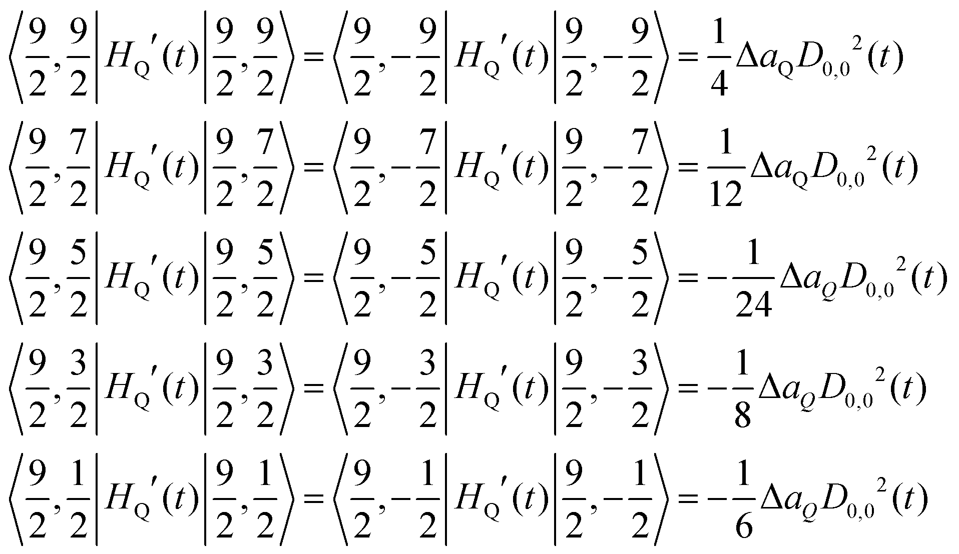

The elements of the HQ′(S) matrix below the diagonal are given as 〈m|HQ(S)|n〉 = 〈n|HQ(S)|m〉*, where “*” denotes complex conjugation. Other elements are equal to zero. The Wigner rotation matrices47,48 depend on time via stochastic fluctuations of the angle Ω(t) describing the orientation of the principal axis system of the perturbing Hamiltonian with respect to the principal axis system of the main Hamiltonian: D0,m2(t) ≡ D0,m2(Ω(t)).
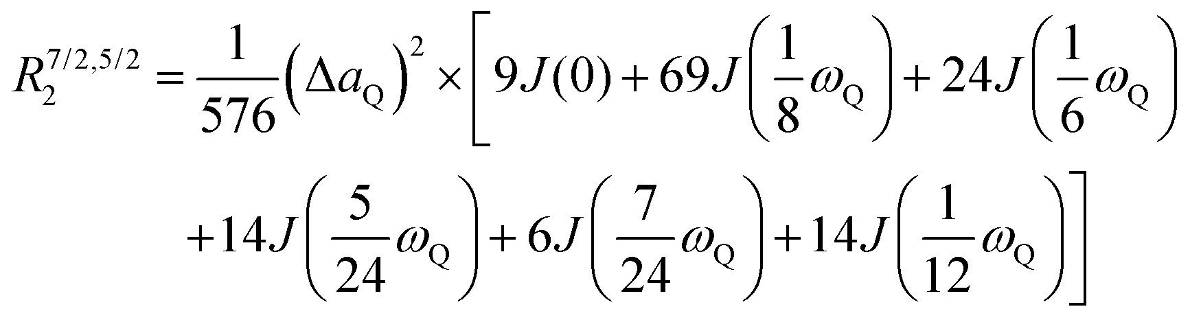
Expressions for the relaxation rates
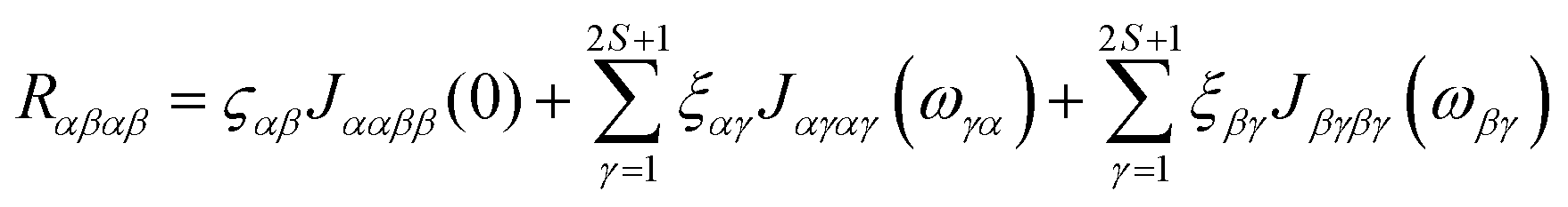
According to the Redfield relaxation theory the relaxation rates measured in the NQR experiment correspond to the relaxation coefficients Rαβαβ. They are given as linear combinations of “generalized” spectral density functions![[J with combining tilde]](https://www.rsc.org/images/entities/i_char_004a_0303.gif) (ω):40,42–44
(ω):40,42–44The
 ααββ(ω) quantities are determined as:
where the spectral density J(ω) is given as:

Thus, the formula for Rαβαβ can be rewritten in the form suitable for practical calculations:

The coefficients ςαβ, ξαγ can be expressed by the coefficients aα,i and aβ,i for the eigenstates |ψα〉 and |ψβ〉, respectively. Their explicit form for S = 9/2 are given below:


Acknowledgements
This project has received funding from the European Union's Horizon 2020 research and innovation programme under grant agreement no. 665172.References
- P. Caravan, J. J. Ellison, T. J. McMurry and R. B. Lauffer, Chem. Rev., 1999, 99, 2293 CrossRef PubMed.
- É. Tóth, L. Helm and A. E. Merbach, Relaxivity of MRI Contrast Agents, in Contrast Agents I, ed. W. Krause, Springer, Berlin, 2002, pp. 61–101 Search PubMed.
- P. Caravan, Chem. Soc. Rev., 2006, 35, 512 RSC.
- I. Bertini, C. Luchinat and G. Parigi, Adv. Inorg. Chem., 2005, 57, 105 CrossRef.
- A. S. Merbach, L. Helm and É. Tóth, The Chemistry of Contrast Agents in Medical Magnetic Resonance Imaging, Wiley & Sons. Ltd, United Kingdom, 2013 Search PubMed.
- I. Bertini, O. Galas, C. Luchinat and G. Parigi, J. Magn. Reson., Ser. A, 1995, 113, 151 CrossRef.
- T. Nilsson, J. Svoboda, P.-O. Westlund and J. Kowalewski, J. Chem. Phys., 1998, 109, 6364 CrossRef.
- D. Kruk, T. Nilsson and J. Kowalewski, Phys. Chem. Chem. Phys., 2001, 3, 4907 RSC.
- D. Kruk and J. Kowalewski, Mol. Phys., 2003, 101, 2861 CrossRef.
- J. Kowalewski, D. Kruk and G. Parigi, Adv. Inorg. Chem., 2005, 57, 41 CrossRef.
- E. Belorizky, P. H. Fries, L. Helm, J. Kowalewski, D. Kruk, R. R. Sharp and P.-O. Westlund, J. Chem. Phys., 2008, 128, 052315 CrossRef PubMed.
- F. Winter and R. Kimmich, Biophys. J., 1985, 28, 331 CrossRef.
- P.-O. Westlund, Phys. Chem. Chem. Phys., 2010, 12, 3136 RSC.
- D. Kruk, A. Kubica, W. Masierak, A. F. Privalov, M. Wojciechowski and W. Medycki, Solid State Nucl. Magn. Reson., 2011, 40, 114 CrossRef PubMed.
- M. Florek-Wojciechowska, M. Wojciechowski, R. Jakubas, S. Brym and D. Kruk, J. Chem. Phys., 2016, 144, 054501 CrossRef PubMed.
- M. Florek-Wojciechowska, R. Jakubas and D. Kruk, Phys. Chem. Chem. Phys., 2017, 19, 11197 RSC.
- M. Nolte, A. Privalov, J. Altmann, V. Anferov and F. Fujara, J. Phys. D: Appl. Phys., 2002, 35, 939 CrossRef.
- D. Kruk, J. Altmann, F. Fujara, A. Gädke, M. Nolte and A. F. Privalov, J. Phys.: Condens. Matter, 2005, 17, 519 CrossRef.
- D. Kruk and O. Lips, Solid State Nucl. Magn. Reson., 2005, 28, 180 CrossRef PubMed.
- D. Kruk and O. Lips, J. Magn. Reson., 2006, 179, 250 CrossRef PubMed.
- P.-O. Westlund, J. Chem. Phys., 1998, 108, 4945 CrossRef.
- I. Bertini, J. Kowalewski, C. Luchinat, T. Nilsson and G. Parigi, J. Chem. Phys., 1999, 111, 5795 CrossRef.
- R. R. Sharp and L. Lohr, J. Chem. Phys., 2001, 115, 5005 CrossRef.
- R. R. Sharp, J. Magn. Reson., 2002, 154, 269 CrossRef PubMed.
- D. Kruk, T. Nilsson and J. Kowalewski, Mol. Phys., 2001, 99, 1435 CrossRef.
- D. Kruk and J. Kowalewski, J. Chem. Phys., 2009, 130, 174104 CrossRef PubMed.
- M. Rubinstein, A. Baram and Z. Luz, Mol. Phys., 1971, 20, 67 CrossRef.
- B. Halle and H. Wennerström, J. Magn. Reson., 1981, 44, 89 Search PubMed.
- P.-O. Westlund, Mol. Phys., 1995, 85, 1165 CrossRef.
- P.-O. Westlund, N. Benetis and H. Wennerström, Mol. Phys., 1987, 61, 177 CrossRef.
- D. Kruk, J. Kowalewski, D. S. Tipikin, J. H. Freed, M. Mościcki, A. Mielczarek and M. Port, J. Chem. Phys., 2011, 134, 024508 CrossRef PubMed.
- N. Okubo, I. Mutsuo and Y. Ryozo, Z. Naturforsch., A: Phys. Sci., 1995, 50, 737 Search PubMed.
- N. Okubo, H. Sekiya, C. Ishikawa and Y. Abe, Z. Naturforsch., A: Phys. Sci., 1992, 47, 713 Search PubMed.
- N. Okubo and Y. Abe, Z. Naturforsch., A: Phys. Sci., 1994, 49, 680 Search PubMed.
- L. T. A. Ho and L. F. Chibotaru, Phys. Rev. B, 2018, 97, 024427 CrossRef.
- J. Van Kranendonk and M. Walker, Phys. Rev. Lett., 1967, 18, 701 CrossRef.
- R. C. Zamar and C. E. Gonzales, Phys. Rev. B: Condens. Matter Mater. Phys., 1995, 51, 932 CrossRef.
- A. Borel, R. B. Clarkson and R. L. Belford, J. Chem. Phys., 2007, 126, 054510 CrossRef PubMed.
- S. Reschke, Z. Wang, F. Mayr, E. Ruff, P. Lunkenheimer, V. Tsurkan and A. Loidl, Phys. Rev. B, 2017, 96, 144418 CrossRef.
- C. P. Slichter, Principles of magnetic resonance, Springer-Verlag, 1990 Search PubMed.
- R. Kimmich, NMR: Tomography, Diffusometry, Relaxometry, Springer, 2012 Search PubMed.
- D. Kruk, Understanding Spin Dynamics, Pan Stanford Publishing Pte. Ltd, Singapore, 2016 Search PubMed.
- A. Redfield, Encyclopedia of Nuclear Magnetic Resonance, ed. D. Grant and R. Harris, Wiley & Sons. Ltd, England, 2002 Search PubMed.
- J. Kowalewski and L. Maler, Nuclear Spin Relaxation in Liquids: Theory, Experiments, and Applications, Taylor & Francis, Florida, 2006 Search PubMed.
- H. Scharfetter, J. Magn. Reson., 2016, 271, 90 CrossRef PubMed.
- H. Scharfetter, M. Bödenler and D. Narnhofer, J. Magn. Reson., 2018, 286, 148 CrossRef PubMed.
- D. M. Brink and S. G. Satchler, Angular Momentum, Oxford University Press Inc., New York, 1993 Search PubMed.
- A. R. Edmonds, Angular Momentum in Quantum Mechanics, Princeton University Press, Princeton, 1974 Search PubMed.
| This journal is © the Owner Societies 2018 |