Langevin behavior of the dielectric decrement in ionic liquid water mixtures†
Received
3rd April 2018
, Accepted 16th May 2018
First published on 17th May 2018
Abstract
We present large scale polarizable simulations of mixtures of the ionic liquids 1-ethyl-3-methylimidazolium trifluoromethanesulfonate and 1-ethyl-3-methylimidazolium dicyanamide with water, where the dielectric spectra, the ion hydration and the conductivity were evaluated. The dielectric decrement, the depression of the dielectric constant of water upon addition of ions, is found to follow a universal functional of Langevin type. Only three physical properties need to be known to describe the complete range of possible concentrations, namely the dielectric constant of pure water, of pure ionic liquid and the linear slope of the dielectric decrement at low ionic liquid concentrations. Both the generalized dielectric constant, as well as the water contribution to the dielectric permittivity follow the functional dependence. We furthermore find that a scaling of van der Waals parameters upon addition of polarizable forces to the force field is necessary to correctly describe the frequency dependent dielectric conductivity and its contribution to the dielectric spectrum, as well as the static electric conductivity, which is also treated in the framework of a pseudolattice theory.
1 Introduction
Knowledge of the electric and dielectric properties of pure ionic liquids and their binary mixtures are of immediate interest to many ionic liquid applications involving electrochemical processes. Of main concern is the interaction of ions and dipoles with an applied electric field, which comprises the electric and dielectric conductivity of ions and the collective reorientation of dipoles. The electric conductivity of an electrolyte solution is a function of both the number of charge carriers, and their respective mobility. Although pure ionic liquids feature a maximum number of ions, the conductivity is low due to their high viscosity. The addition of even small fractions of solvent (here water) decreases the viscosity drastically.1,2 Consequently, the conductivity of aqueous ionic liquid systems exhibits a parabolic dependence on ionic liquid concentration.2–5 At low ion concentrations the Debye–Hückel–Onsager theory, which is based on the existence of ionic atmospheres, is capable of describing the electric conductivity of ionic solutions.6–12 However, at high concentrations this ionic atmosphere paradigm breaks down (e.g. only one ion forms the atmosphere at 0.01 M ionic concentration), the structure of an ionic solution changes and is best described by a pseudolattice.2,4,13,14 The conductivity of ionic liquid/solvent mixtures based on the pseudolattice model of independent low and high mobility cells and uncorrelated ion jumps leads to a universal, parameter-free, parabolic relation between the normalized conductivity and the reduced concentration.4 Deviations of the conductivity of highly concentrated solutions from the universal curve arise from specific ion–ion, ion–solvent and solvent–solvent interactions, giving rise to heterogeneous cell distributions and correlated ion jumps.2
Dielectric relaxation spectroscopy (DRS) of ionic solutions opens up the possibility of quantifying ion–ion and ion–solvent interactions.15 DRS is a prevalent technique to study relaxation in amorphous systems and in particular liquids.15–17 Dielectric experiments probe the complete sample measuring collective translational and rotational motion governed by electrostatic forces. Frequently, the collectivity hinders the interpretation of dielectric data due to the overlap of various contributions and additional effects, e.g. hydrogen bonding, interionic vibrations and rotations as well as ion-cloud relaxations.15,18 As simulation studies may provide these contributions separately, a computational spectrum can be gradually assembled bottom-up enabling a physically meaningful interpretation of the underlying processes.18,19
One of the key quantities of a solvent is its static dielectric permittivity ε(0), the real part of the dielectric spectrum at zero frequency.20 In mixtures of two non-ionic compounds j and k several mixing rules for the static dielectric permittivity ε(ω = 0,Φj) as a function of volume fraction Φj of the respective compounds with static dielectric permittivities εj(0) and εk(0) have been reported. For reasons of readability, we write in the following ε(Φj) instead of ε(ω = 0,Φj), referring always to the zero-frequency limit of ε, unless stated otherwise. A common mixing rule is
| | | ε(Φj)ξ = Φj·(εj)ξ + (1 − Φj)·(εk)ξ | (1) |
with exponent
ξ having values of 1, 1/2 or 1/3.
17,21–24 An exponent of 1/3 with variations of
eqn (1) is also used by Bruggeman,
25 as well as Cohen and coworkers.
26 Furthermore, Pujari
et al.27 suggested a logarithmic partitioning of the dielectric constants of the pure compounds
| | ln![[thin space (1/6-em)]](https://www.rsc.org/images/entities/char_2009.gif) ε(Φj) = Φjlnεj + (1 − Φj)lnεk ε(Φj) = Φjlnεj + (1 − Φj)lnεk | (2) |
which reproduced the static generalized dielectric constant of our non-polarizable aqueous mixture of 1-butyl-3-methylimidazolium tetrafluoroborate.
28 However, strictly speaking, these mixing rules are valid for the mixture of neutral components which is not the case for electrolyte solutions such as aqueous ionic liquid mixtures. Adding simple (atomic) salts to water leads to a decrease of the dielectric constant. At small ion concentration, the decrease is a linear function of the ion concentration.
29 At higher concentrations, non-linear effects are observed. A systematic study of several electrolyte theories was reported by Thomsen and co-workers.
30 A number of theories have been developed to characterize this so-called dielectric decrement. In principle, dielectric saturation is caused by the strong interaction between solvent dipoles and the electric field surrounding the ions where the dielectric constant shows a Langevin type behavior on the (scaled) electric field.
17,31,32 Gavish and Promislow
33 recently reported that experimental static dielectric constants of various electrolytes also show a Langevin type dependence, but with respect to the salt concentration
csalt. Using a phenomenological microfield approach, Gavish and Promislow arrived at
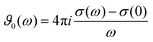
| | 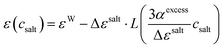 | (3) |
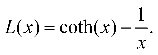
with the Langevin function
L(
x)
| | 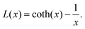 | (4) |
Starting at the dielectric constant of pure water
εW the salt decreases the dielectric constant
ε(
csalt) by Δ
εsalt to a hypothetical minimum dielectric constant
εMS at
csalt → ∞. Thus, Δ
εsalt =
εW −
εMS. Here, the artificial high concentration limit
εMS is a fit parameter, and has no direct physical meaning. The quantity
αexcess can be fitted from the slope at small concentrations. Levy
et al. investigated interactions of water dipoles in the vicinity of ions by a static dipolar Poisson–Boltzmann approach.
34 They were able to reproduce the dielectric decrement up to ion concentrations of 5 M. Their model was also successful for our non-polarizable aqueous 1-butyl-3-methylimidazolium tetrafluoroborate mixtures.
28 More recently, Persson proposed a description of the dielectric decrement of simple salt solutions
via dressed-ion theory, where the electrostatic screening through ion correlations acts similar to a reduction of the ionic charge.
35 However, the applicability of the diverse models for the dielectric decrement of simple salts to aqueous ionic liquid mixtures is questionable. An atomic salt only contributes to the translational part of the dielectric spectrum
via the dielectric conductivity. The large molecular ions in an ionic liquid, however, contribute both to the translational and rotational processes, since they carry not only a charge, but also a molecular dipole moment. This study therefore contributes to the understanding of the dielectric decrement in ionic liquid/water mixtures, and the extent to which atomic ion model theories apply to molecular ions.
Recently, we have studied by classical molecular dynamics simulation the structure, coordination, hydrogen bonding and dielectric spectra of aqueous mixtures of 1-butyl-3-methylimidazolium tetrafluoroborate28,36–38 and 1-ethyl-3-methylimidazolium trifluoromethanesulfonate19,39 as a function of the ionic liquid concentration. However, we have noticed that polarizable forces are important to reproduce experimental spectra in the case of ionic liquids,19 but not so much for water.40 To our best knowledge, the present work is the first polarizable molecular dynamics simulation to compute and analyze dielectric spectra of ionic liquid/water mixtures. The computer simulation of the complex dielectric spectra of ionic liquid/water mixtures enables the direct decomposition into contributions from εIL (ionic liquid) and εW (water), as well as the translational part of the dielectric spectrum, ϑ0. Furthermore, the number of hydrated water molecules is directly accessible via Voronoi tessellation.41 The computational dielectric decrement as a function of ionic liquid concentration is compared to different model theories. We find that a universal Langevin functional, taking into account the static dielectric constant of pure water and ionic liquid, as well as the initial slope of the dielectric decrement at low concentrations is capable of describing the dielectric decrement. No further fit parameters are required. In addition, we test the applicability of simple volume-based mixing of the pure dielectric constants of water and the pure ionic liquid, as well as one fitting parameter (the dielectric constant of hydration water). Finally, we calculate the corrected universal conductivity parabola of the electric conductivity, thus interrogating the pseudolattice model for the conductivity of ionic liquids.2,4
2 Methods
The aqueous mixtures of the ionic liquids 1-ethyl-3-methylimidazolium trifluoromethanesulfonate [C2mim][OTf] and 1-ethyl-3-methylimidazolium dicyanamide [C2mim][N(CN)2] at various concentrations were studied by polarizable molecular dynamics simulations.
2.1 Force field
The polarizable water model SWM4 was taken from literature.42 Due to the importance to correctly model the interactions of the ionic liquid ions with water, the force field parameterization of C2mim+, OTf− and N(CN)2− was performed with GAAMP,43 an automated force field parameterization tool which takes explicitly the compound–water interactions into account. Starting from CGenFF parameters,44,45 quantum-mechanical data are used to verify and adjust equilibrium bond length and angle parameters. It detects and handles soft dihedrals with low energy barriers resulting in conformational changes of molecules. The Lennard-Jones interactions between the first and last atom of all dihedrals are scaled by a factor of 0.5. Furthermore, it assigns partial charges and polarizabilities according to the interaction with a test charge of q = 0.5 e at various grid positions around the target molecule. This way, solvation free energies can be reproduced with promising accuracy.43 All force field parameters are given in the ESI.†
The induced dipoles during the molecular dynamics simulation are represented by additional Drude particles with a mass of 0.2 u which is subtracted from the mass of the attached polarizable atom. Hydrogen atoms are left non-polarizable. The force constant of the bond of the Drude particle to the polarizable atom is set uniformly to 500 kcal (mol Å2)−1.
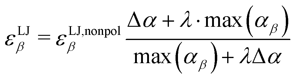
As the attractive part of the van der Waals interaction is described by the interaction of the induced dipoles, the well depths of the Lennard-Jones potential, εLJβ, of each atom β have to be adjusted in order not to count the dispersion twice
| | 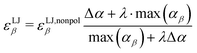 | (5) |
where Δ
α = max(
αβ) −
αβ. This empirical reduction of Vlugt and co-workers
46 ensures that non-polarizable atoms,
e.g. hydrogens in our Drude-model, are unaffected by the scaling. The parameter
λ varies between 0 and 1 and describes the relative importance of the Lennard-Jones parameter
εLJβ for the dispersion in the simulation. A value of 1 corresponds to full Lennard-Jones description of dispersion. A hypothetical
λ-value of zero results for the atom
β with the largest polarizability max(
αβ) in an abandoning of Lennard-Jones interactions for this atom and all non-charged intermolecular interactions of this atom are modeled by the interaction of the respective induced dipoles. Thus, the Lennard-Jones parameter of the atom with the largest polarizability, max(
αβ), is scaled by
λ, and all other atoms by a factor between
λ and 1 depending on their polarizability. We evaluated the density and electric conductivity of the pure ionic liquids [C
2mim][OTf] and [C
2mim][N(CN)
2] with
λ ranging from 0.3 to 1,
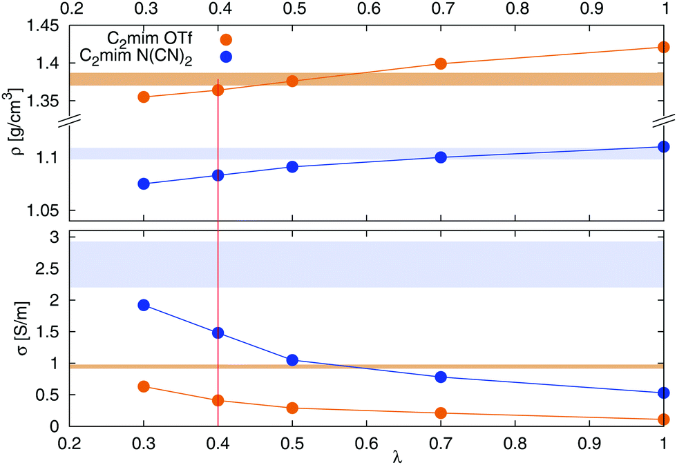
Fig. 1. A decrease of
λ leads to a decrease in density, as well as an increase in conductivity. A value of
λ = 0.4 was chosen for all further simulations, since it results in a reasonable compromise between a correct density and conductivity.
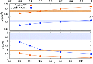 |
| | Fig. 1 Dependence of density (top) and conductivity (bottom) of [C2mim][OTf] (orange) and [C2mim][N(CN)2] (blue) on the scaling of van der Waals interactions via the parameter λ according to eqn (5). The colored area corresponds to the range of experimental densities47 and conductivities.48–53 | |
2.2 Computational setup
The number of ion pairs of the two ionic liquids under investigation was varied from 50 to 1000 in a box of roughly 70 Å and filled with water molecules to yield ionic liquid concentrations ranging from 0.25 M up to the concentrated ionic liquids with cIL of 5.2 M and 6.1 M in case of [C2mim][OTf] and [C2mim][N(CN)2], respectively. The exact number of ion pairs, water molecules and the resulting concentrations are listed in Table 1.
Table 1 Average coordination numbers of cations and anions, volume distribution between the components, and percentage of direct ion pairs (CIP) and mediated ion pairs with one (SIP) or two (2SIP) water molecules between the ions
| IL |
N
IL
|
N
H2O
|
c
IL [M] |
Volume occupancy |
Coordination number |
Z
|
Ion pairs |
|
ϕ
IL
|
ϕ
bulk
|
ϕ
Chyd
|
ϕ
Ahyd
|
ϕ
hyd
|
C–C |
C–A |
C–W |
A–A |
A–W |
CIP (%) |
SIP (%) |
2SIP (%) |
#CIP |
| [C2mim][OTf] |
50 |
10550 |
0.25 |
0.05 |
0.69 |
0.17 |
0.12 |
0.26 |
0.2 |
0.5 |
40 |
0.1 |
28 |
58 |
46 |
43 |
11 |
1.2 |
| 100 |
10029 |
0.50 |
0.09 |
0.46 |
0.31 |
0.22 |
0.45 |
0.3 |
1.0 |
38 |
0.3 |
27 |
49 |
67 |
29 |
3 |
1.4 |
| 200 |
8988 |
1.00 |
0.19 |
0.18 |
0.50 |
0.36 |
0.63 |
0.9 |
1.8 |
36 |
0.6 |
24 |
35 |
89 |
11 |
0 |
2.0 |
| 400 |
6907 |
2.01 |
0.37 |
0.01 |
0.58 |
0.46 |
0.61 |
2.3 |
3.3 |
30 |
1.5 |
18 |
17 |
99 |
1 |
0 |
2.0 |
| 600 |
4825 |
3.02 |
0.56 |
0.00 |
0.44 |
0.39 |
0.44 |
4.3 |
4.8 |
22 |
2.4 |
13 |
8 |
100 |
0 |
0 |
4.8 |
| 800 |
2744 |
4.01 |
0.75 |
0.00 |
0.25 |
0.24 |
0.25 |
6.9 |
6.3 |
13 |
3.3 |
7.1 |
3 |
100 |
0 |
0 |
6.3 |
|
|
| [C2mim][N(CN)2] |
50 |
10648 |
0.25 |
0.04 |
0.73 |
0.17 |
0.09 |
0.23 |
0.2 |
0.7 |
40 |
0.1 |
20 |
51 |
55 |
32 |
13 |
1.2 |
| 100 |
10226 |
0.50 |
0.08 |
0.53 |
0.31 |
0.16 |
0.39 |
0.4 |
1.1 |
38 |
0.2 |
19 |
43 |
71 |
24 |
4 |
1.5 |
| 200 |
9382 |
0.99 |
0.16 |
0.27 |
0.49 |
0.28 |
0.57 |
1.0 |
1.7 |
36 |
0.4 |
17 |
32 |
89 |
11 |
1 |
2.0 |
| 400 |
7694 |
1.95 |
0.32 |
0.04 |
0.61 |
0.41 |
0.64 |
2.4 |
2.8 |
31 |
0.7 |
14 |
18 |
98 |
2 |
0 |
2.8 |
| 600 |
4825 |
2.90 |
0.47 |
0.00 |
0.52 |
0.44 |
0.52 |
4.3 |
3.8 |
26 |
1.0 |
11 |
10 |
100 |
0 |
0 |
3.8 |
| 800 |
4318 |
3.83 |
0.63 |
0.00 |
0.37 |
0.38 |
0.37 |
6.5 |
4.9 |
19 |
1.2 |
8.0 |
5 |
100 |
0 |
0 |
4.9 |
| 900 |
2000 |
4.91 |
0.80 |
0.00 |
0.20 |
0.23 |
0.20 |
9.1 |
6.2 |
10 |
1.5 |
4.4 |
2 |
100 |
0 |
0 |
6.2 |
The starting configurations for each system were mostly taken from previous calculations without scaling of the Lennard-Jones parameters, and thus pre-equilibrated. After a NPT equilibration run of at least 1 ns for each system (p = 1 atm), and a NVT equilibration run of at least 1 ns, normal trajectory production (NVT ensemble) was performed for at least 40 ns with a time step of 0.5 fs. We use the extended Lagrange formalism54 with a dual Nosé–Hoover thermostat,55,56 where non-Drude particles are kept close to 300 K, and Drude particles at 1 K. The configurations were saved each 25 fs. For the last 1 ns the frequency to store the configurations and velocities was reduced to 5 fs to compute current auto-correlation functions 〈J(0)·J(t)〉.
Electrostatic interactions were calculated using the Particle-Mesh Ewald method with a cut-off of 14 Å and an Ewald parameter of κ = 0.41 Å−1. Bond lengths of bonds involving hydrogens were kept fixed using SHAKE.
3 Theory
3.1 Computation of the generalized dielectric constant
The collective relaxation of neutral molecules and molecular ions featuring a dipole moment comprises the rotational response, the permittivity ε(ω), of the overall liquid.57 In contrast, only the translation of atomic or molecular ions (but not neutral molecules) contribute to the translational part ϑ0(ω) of the dielectric spectrum directly.18 Polar non-charged mixtures have zero values for ϑ0(ω) at all frequencies. Adding a simple salt (without a molecular dipole) to a liquid results in a permittivity ε(ω) solely from the liquid and a dielectric conductivity ϑ0(ω) from the salt. In aqueous solutions of atomic salts the rotational and translational dielectric peaks of the generalized dielectric constant Σ0(ω) can be separated on the frequency scale: the former emerge from dipole relaxation of the neutral liquid in the GHz regime whereas the latter are caused by the motion of the ions and are thus located at higher frequency and possess lower amplitudes. However, ionic liquids are of particular interest as they possess a molecular dipole (therefore contributing to ε(ω)) and carry a charge (contributing to the dielectric conductivity ϑ0(ω)) resulting in a stronger coupling between translational and rotational dielectric relaxation.18 Consequently, ionic liquids and their mixtures are ideal test systems to study dielectric theories.16,17,30,31,58 However, as the molecular ions are neither of spherical nor ellipsoid shape, inclusion theories described in review articles59,60 are not part of the current study as they also assume homogeneous mixtures whereas ionic liquids are known to form polar and apolar nanostructures.61,62
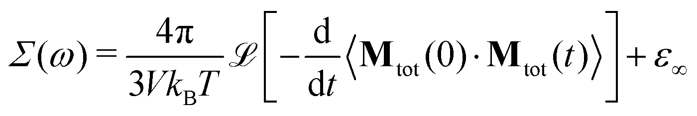
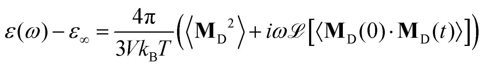
The generalized dielectric constant Σ(ω) can be evaluated from equilibrium molecular dynamics simulations39,63via the Laplace transform (![[script L]](https://www.rsc.org/images/entities/char_e144.gif) […]) of the auto-correlation function of the total collective dipole moment Mtot(t) at temperature T and system volume V
[…]) of the auto-correlation function of the total collective dipole moment Mtot(t) at temperature T and system volume V
| |  | (6) |
We use the CGS system of units, instead of SI notation. Thus, the generalized dielectric constant, as well as all dielectric properties in the following are in units of 4π
εvac with vacuum permittivity of
εvac = 8.85 × 10
−12 A s V
−1 m
−1.
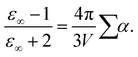
In contrast to non-polarizable simulations with a high-frequency limit of the dielectric constant of ε∞ = 1, the finite value of ε∞ in polarizable molecular dynamics simulations depends approximately on the sum of polarizabilities, as characterized by the Clausius–Mossotti relation
| |  | (7) |
As the collective dipole moment
Mtot(
t) suffers from jumps of charged molecules due to periodic boundary conditions,
39 a decomposition into a sum of the rotational,
MD(
t), and translational part,
MJ(
t) is of practical use.
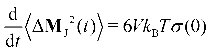
The slope of the mean-squared displacement of MJ(t) yields the static conductivity σ(0) of the liquid
| | 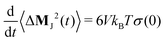 | (8) |
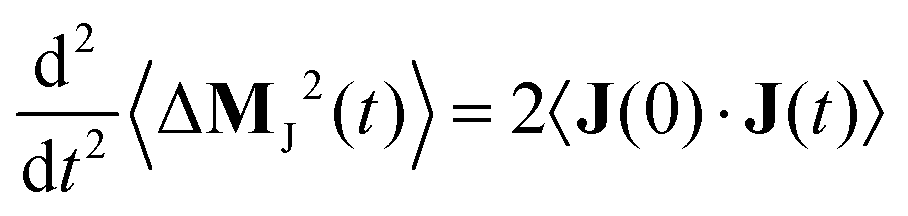
and its second derivative equals twice the electric current auto-correlation function of the electric current
J(
t)
| |  | (9) |
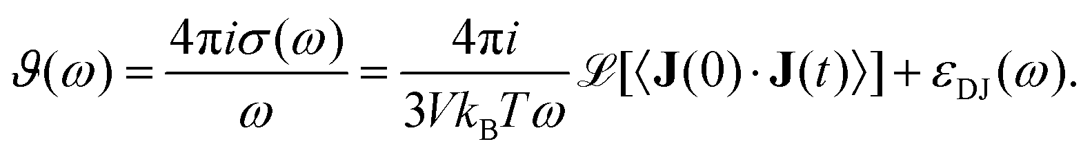
which enters the dielectric conductivity
ϑ(
ω)
| |  | (10) |
The dielectric conductivity
ϑ(
ω) is the translational contribution to
Σ(
ω) and differs from the frequency dependent conductivity
σ(
ω).
63 Since 〈Δ
MJ2(
t)〉 uses the unfolded trajectory and
J(
t) depends on the velocity but not position of the charged molecules, the periodic boundary problem of jumping ions for the computation of
MJ(
t) is solved. The cross-coupling
εDJ(
ω) between rotation and translation in principle contributes to
ϑ(
ω), however we find that
εDJ(
ω) is negligibly small in the current study, thus it is omitted from all further discussions.
The remaining part of the collective dipole moment concerns the rotation of the molecules, MD(t). Here, both charged and neutral molecules contribute but on different frequency regimes. The total dielectric permittivity ε(ω) is
| |  | (11) |
where we again assume
εDJ(
ω) ≃ 0. The total dielectric permittivity can be decomposed into contributions from each molecular species
j| | 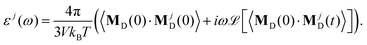 | (12) |
Here, the collective rotational dipole moment
MjD(
t) is correlated with the total rotational dipole moment
MD(
t) to include all possible rotational couplings between the various molecular species. In principle, the decomposition into contributions from permanent and induced dipoles is also possible. However, as we showed for pure [C
2mim][OTf], the relaxation of the induced dipoles happens more or less at the same frequency regions as the permanent dipolar relaxation and is not restricted to higher frequencies.
19 The impact of polarizability on ionic liquids is more fundamental. Coulomb interactions are reduced and dispersion increased.
64
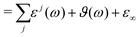
Overall, the generalized dielectric constant Σ(ω) comprises all these contributions, i.e.
| | | Σ(ω) = ε(ω) − ε∞ + ϑ(ω) + ε∞ | (13) |
| |  | (14) |
Since the liquid under investigation contains conducting species, the generalized dielectric constant diverges at zero frequency in experiment and simulation. Consequently, this divergence is removed in experimental and computational dielectric spectra by subtracting the conductivity hyperbola
| |  | (15) |
| | | Σ0(ω) = ε(ω) − ε∞ + ϑ0(ω) + ε∞ | (16) |
indicated by the index 0.
4 Results and discussion
4.1 Ion hydration and association
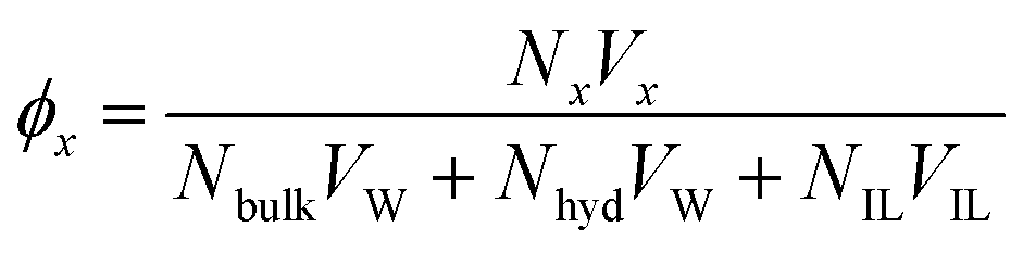
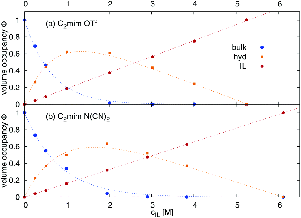
The volume occupancies of the ionic liquid ions (ϕIL), the water molecules in the first solvation shell of at least one ion (= hydration water, ϕhyd) and the remaining water (= bulk water, ϕbulk) are given in Table 1, column ‘volume occupancy’ and depicted in Fig. 2. The volume fractions ϕx are calculated as| |  | (17) |
where x represents the contribution from bulk water, hydration water or ionic liquid respectively. The number of molecules Nx and the average volume per molecule Vx were computed by Voronoi tessellation.41Vx denotes the volume of one molecule of the species x, here 307.8 Å3 for [C2mim][OTf], 270.2 Å3 for [C2mim][N(CN)2], and 29.9 Å3 for H2O (bulk and hydration water). The volume occupancy of bulk water (Fig. 2, blue line) undergoes an exponential decay with increasing ionic liquid concentration as predicted in ref. 28. The volume fraction of ionic liquid increases linearly with concentration. Thus, the volume fraction of hydration water, which is ϕhyd = 1 − ϕbulk − ϕIL, goes through a maximum between 1 and 2 M, before it falls to zero as the overall water content approaches zero. The volume fraction of ϕhyd is employed later to estimate the dielectric constants of water at different ionic liquid concentrations. Table 1 furthermore lists the volume fraction of hydration water in the first shell of cations (ϕChyd) and anions (ϕAhyd). The percentage of water molecules which are simultaneously in the hydration shell of a cation and an anion (evaluated via (ϕChyd + ϕAhyd − ϕhyd)/ϕhyd) increases with increasing ionic liquid content of the mixture.
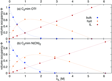 |
| | Fig. 2 Volume distribution between ionic liquid, hydration and bulk water calculated viaeqn (17). | |
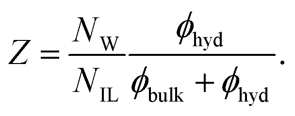
The average coordination number of the cations and anions are also listed in Table 1, column ‘coordination-number’. The number of ion contacts (cation–cation, C–C and cation–anion C–A) increases with increasing ion concentration, whereas the ion hydration number (cation–water, C–W and anion–water, A–W) decreases. This behavior is also reflected in the number of bound solvent molecules per ion pair, Z, computed as
| | 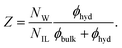 | (18) |
The number of hydration water molecules per ion pair decreases with increasing ionic liquid concentration. Thus, at low concentrations the ions are surrounded mainly by water, but at high concentrations ionic liquid domains form. Indeed, the particular size and shape of these domains which are directly determined by the specific interactions between the ionic liquid and water considerably affect the electrical conductivity of the ionic liquid–water mixtures in this highly concentrated region.
The formation of ionic liquid pairs or domains can be followed easily in computer simulation, as explained in the following. The occurrence of contact ion pairs (CIP) and water mediated ion pairs (SIP and 2SIP), as described by Eigen and Tamm,65 is evaluated via Voronoi tessellation, Table 1, column ‘ion pairs’. In principle, four different configurations of ion pairs are possible. First, no ion pair occurs, the cation and anion are fully hydrated (Yaq− + Xaq+). Second, the hydration shells of the ions touch ([Y−–H2O–H2O–X+]aq), forming a double-solvent-separated ion pair (2SIP). Third, one hydration water of the complex is lost ([Y−–H2O–X+]aq), to form a solvent-shared ion pair (SIP). Fourth, the ions are in direct contact ([Y−–X+]aq), forming a contact ion pair (CIP).15 In the dilute solutions (cIL ≤ 0.5 M), CIP, SIP and 2SIP occur, but no free hydrated ions. Most of the ions involved in a CIP form only one contact ion pair (#CIP in Table 1). However, already at low concentrations a number of ionic liquid ions feature more than one contact ion pair, i.e. form a charged ionic liquid cluster with unequal number of cations and anions. At higher concentrations, nearly all ions form CIP clusters, so that nearly no SIP or 2SIP configurations occur. The number of CIP contacts ranges from two to six for cIL ≥ 1 M, so that the term ‘ion pair’ becomes misleading, since rather ionic liquids domains form, analogous with the known formation of nanostructures in pure ionic liquids.61,62
4.2 Dielectric spectra and dielectric decrement
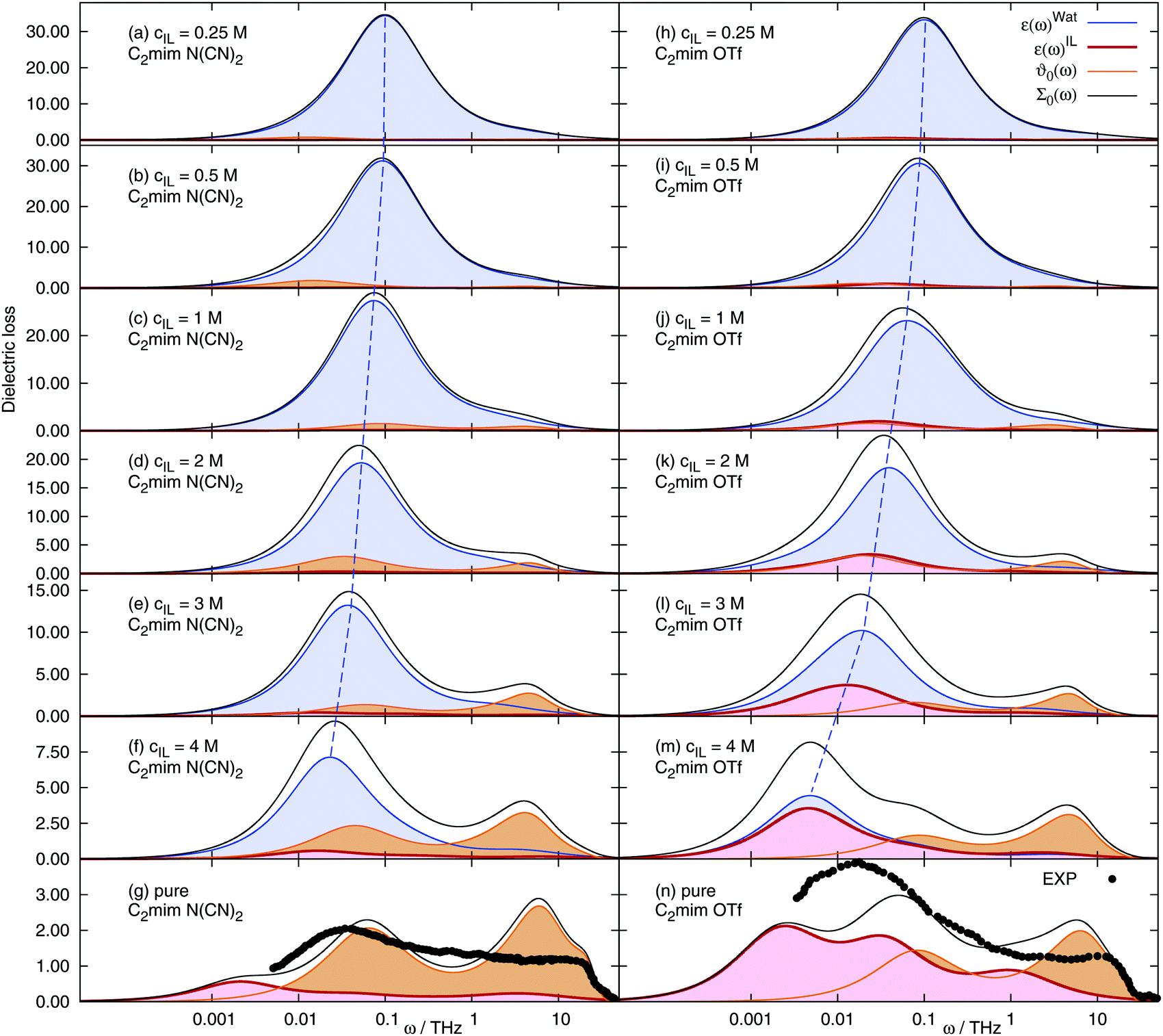
The mean square displacement 〈ΔMJ2(t)〉, the electric current autocorrelation function 〈J(0)J(t)〉 and the rotational contributions to the dielectric permittivity 〈MD(0)MxD(t)〉 (with x being water, cations or anions respectively) were fitted according to the procedure outlined in the Theory section and the ESI.† Thus, the required Laplace transform in eqn (10) and (12) can be done analytically. All fitting parameters are given in the ESI† as well. The dielectric spectra (imaginary part of Σ0(ω)) of the different ionic liquid/water mixtures change significantly with the ionic liquid concentration, Fig. 3. The water peak is shifted to lower frequencies with increasing cIL, since the fraction of fast bulk water, ϕbulk, decreases and the fraction of retarded hydration water, ϕhyd, increases (see Fig. 2), leading to an overall slow down of the observed average water dynamics. Since the conductivity increases with the ionic liquid concentration, the translational contribution ϑ0(ω) to the overall spectrum increases with cIL. The rotational contribution εIL of the ions differs largely between the two studied systems. For [C2mim][N(CN)2] the contribution is very small and increases only slightly with cIL. In contrast, ε(ω)IL of [C2mim ][OTf] contributes significantly to the observed spectrum at concentrations beyond 2 M. For the pure ionic liquids (bottom row of Fig. 3) experimental spectra are also given, as published in ref. 66 andref. 19. The polarizable ionic liquid simulations with scaled Lennard-Jones parameters produces dielectric spectra close to experiment for both [C2mim][OTf] and [C2mim][N(CN)2], although the agreement is not quantitative. An important advantage of our current simulation over previous polarizable simulations without scaling of the dispersion interactions is the correct description of the onset of the shoulder at ω ∼ 25 THz (ν ∼ 4000 GHz) for both systems. It arises nearly quantitatively from the translational contribution ϑ0(ω) to the spectrum. Previously,19 the shoulder was missed, due to the largely underestimated conductivity caused by the overestimation of dispersive forces in the employed IL force fields. However, since the scaling parameter λ was chosen to best match experimental conductivities σ(0) (but not ϑ0(ω)), the translational contribution is overestimated, leading to deviations from experiment at 5–10 THz. Furthermore, the force field was designed to reproduce quantum mechanical data, as well as the interactions between ionic liquid and water and is not particularly optimized towards experimental bulk properties, leading to deviations around 0.01 THz for [C2mim][OTf]. More refined polarizable force fields (but without scaling of the dispersion interactions), were shown to depict the dielectric spectrum in this frequency range well.19
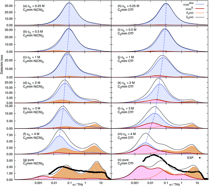 |
| | Fig. 3 Frequency-dependent dielectric spectra of aqueous solutions of 1-ethyl-3-methyl-imidazolium dicyanamide (left) and 1-ethyl-3-methyl-imidazolium trifluoromethanesulfonate (right) at various concentrations. Dashed blue line: mean water frequency. The black dots correspond to experimental dielectric spectra of ref. 66 (C2mim N(CN)2) and ref. 19 (C2mim OTf). | |
The contributions to the static value of the real part of Σ0(ω), namely the ion and water contributions εx, the translational contribution ϑ0 and the high-frequency limit ε∞ are listed in Table 2. The overall dielectric constant Σ0, as well as the water contribution εW decrease with increasing ionic liquid concentration. All other contributions show a more complicated dependence. The dielectric conductivity ϑ0 initially increases with increasing ionic liquid concentration, passes through a maximum at a specific cIL and afterwards decreases again. The ion rotational contributions εC and εA seem to depend both on the ionic liquid concentration (linear) and on an additional term passing through a maximum, which is large for anions, and small/negligible for cations.
Table 2 Dielectric properties of the aqueous ionic liquid mixtures. For the pure water simulation, values were taken from ref. 40 and 67. For water, ε∞ obtained from an overall fit resulted in a slightly higher value than computed by the respective polarizability
| IL |
c
IL [M] |
Σ
0
|
ε
W
|
ε
C
|
ε
A
|
ϑ
0
|
ε
∞
|
| H2O |
0.0 |
78.6 |
77.2 |
0.0 |
0.0 |
0.0 |
1.4 |
|
|
| [C2mim][OTf] |
0.25 |
72.5 |
68.5 |
0.1 |
1.0 |
1.3 |
1.5 |
| 0.50 |
70.6 |
63.9 |
0.2 |
2.0 |
2.9 |
1.5 |
| 1.00 |
64.9 |
54.1 |
0.5 |
3.9 |
4.8 |
1.6 |
| 2.01 |
58.4 |
40.0 |
1.0 |
6.9 |
8.9 |
1.6 |
| 3.02 |
41.0 |
23.9 |
1.1 |
8.0 |
6.2 |
1.7 |
| 4.01 |
28.6 |
10.4 |
1.6 |
7.4 |
7.4 |
1.8 |
| 5.24 |
16.2 |
0.0 |
2.4 |
6.2 |
5.6 |
1.9 |
|
|
| [C2mim][N(CN)2] |
0.25 |
74.7 |
71.1 |
0.1 |
0.0 |
1.9 |
1.5 |
| 0.50 |
70.8 |
64.8 |
0.3 |
0.1 |
4.2 |
1.5 |
| 0.99 |
64.3 |
57.9 |
0.4 |
0.2 |
4.2 |
1.6 |
| 1.95 |
52.6 |
41.6 |
0.8 |
0.4 |
8.2 |
1.6 |
| 2.90 |
37.7 |
28.3 |
1.0 |
0.6 |
6.1 |
1.7 |
| 3.83 |
29.1 |
16.2 |
1.1 |
0.7 |
9.3 |
1.8 |
| 4.91 |
19.8 |
6.5 |
1.4 |
0.8 |
9.3 |
1.9 |
| 6.11 |
12.2 |
0.0 |
1.6 |
0.4 |
8.0 |
2.1 |
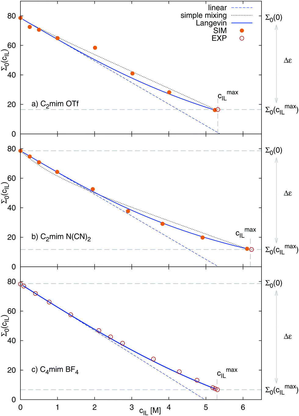
The static dielectric constant Σ0 of the pure ionic liquids equals 16.2 for [C2mim][OTf], which is in good agreement with the experimental value of 16.5.20 For [C2mim][N(CN)2] we obtain a value of 12.2, which is also in fair agreement to the dielectric constant of 11.7 obtained from experiment.68 With increasing water content, the dielectric constants of the ionic liquid/water mixtures approach the value of pure water. The functional dependency of the change in dielectric constant with ionic liquid concentration is linear only for low concentrations, but saturates at higher concentrations. Thus, no linear dependency is observed for the complete concentration range, similar to the known dielectric decrement of electrolyte solutions.
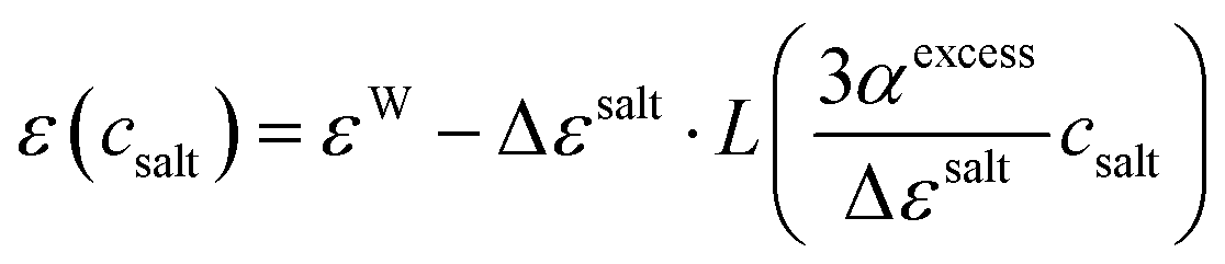
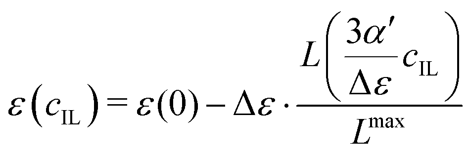
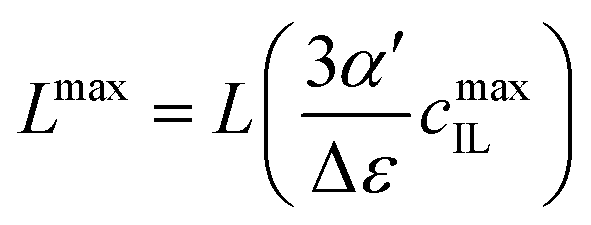
Since the dielectric constant at the maximum possible concentration in ionic liquids is known (in contrast to simple salt solutions), we adapted eqn (3), the formula of Gavish and Promislow, to yield
| |  | (19) |
where the maximum decrement is Δ
ε =
ε(0) −
ε(
cmaxIL). The Langevin function is renormalized by the factor
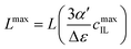
, so that the dielectric constant drops to the known value
ε(
cmaxIL) of the pure ionic liquid at
cmaxIL (instead of the artificial quantity
εMS at
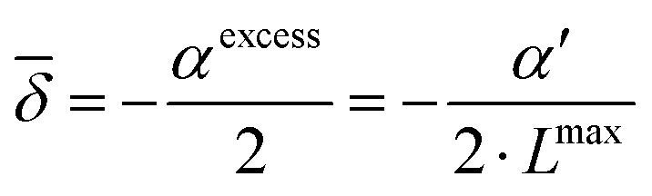
cIL → ∞).
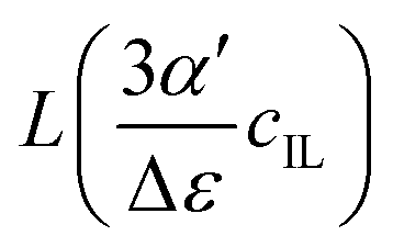
Fig. 4 illustrates the necessity to renormalize the Langevin function using
Lmax. The slope at small concentrations is then
| |  | (20) |
The early work of Collie and coworkers
69 proposed to fit the dielectric constant at small salt concentrations
via| | ε(cIL) = ε(0) + 2![[small delta, Greek, macron]](https://www.rsc.org/images/entities/i_char_e0c5.gif) ·cIL ·cIL | (21) |
where
is related directly to
αexcess and
α′
via| | 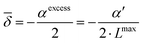 | (22) |
 |
| | Fig. 4 Plot of the Langevin function  . Since the concentration of ionic liquids cannot go beyond the concentration of the pure liquid, cmaxIL, the Langevin function varies between . Since the concentration of ionic liquids cannot go beyond the concentration of the pure liquid, cmaxIL, the Langevin function varies between 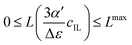 instead of instead of 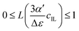 . Renormalization with Lmax resolves the issue. . Renormalization with Lmax resolves the issue. | |
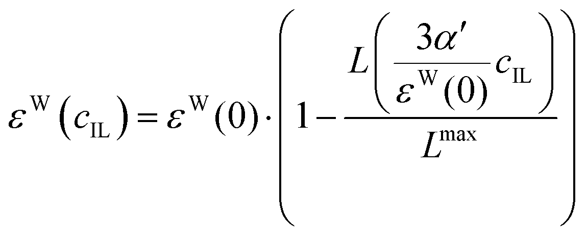
We apply these formulas to aqueous ionic liquid mixtures. Here, the dielectric permittivity of water is accompanied by the dielectric conductivity ϑ0(ω), as well as the dielectric permittivities of the molecular ions resulting in the generalized dielectric constant Σ0(ω). The system of a simple salt dissolved in a solvent employed for the Gavish and Promislow model takes into account only εW, and a nearly negligible contribution of ϑ0. In ionic liquids, however, ϑ0 and the additional components εC and εA also contribute to the generalized dielectric constant. Strictly speaking, we can therefore apply the formula only to the dielectric permittivity of water εW(cIL) where ΔεW = εW(0) − εW(cmaxIL) = εW(0), resulting in
| | 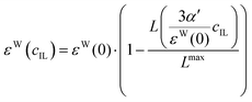 | (23) |
Since the contributions of
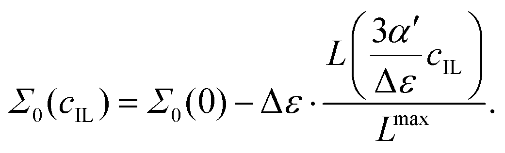
εC and
εA are small, the formula applies (although with less accuracy) to the generalized dielectric constant, too, where Δ
ε =
Σ0(0) −
Σ0(
cmaxIL) to yield
| | 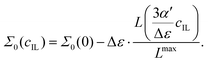 | (24) |
Fig. 5 shows the dielectric constants at various IL concentrations, as well as different functional dependencies. At low concentrations, a linear behavior, eqn (21), can be assumed. The slope at cIL ≤ 1 M is listed in Table 3 as αexcess. For both ionic liquids αexcess ∼ 15 M−1 and δ ∼ −7 M−1 which corresponds to most salts with single charged ions in ref. 69, e.g. LiCl, KF, NaI or KI. At concentrations beyond 2 M, the dielectric constants deviate from linear behavior and can be described without any further fit parameters using eqn (24). The dielectric constants at cIL = 0 (pure water) and cIL = cmaxIL (pure ionic liquid) are known (Table 2) and α′ can be numerically calculated from the slope of the dielectric decrement at low concentrations, αexcessviaeqn (20). The respective α′ for both systems are given in Table 3. The resulting functional dependency of Σ0 with ionic liquid concentration is shown in Fig. 5 as solid line. The dielectric constants over the complete concentration range are well described assuming Langevin-type behavior. To further prove our concept, we describe the experimental dielectric constants70 of 1-butyl-3-methylimidazolium tetrafluoroborate, [C4mim][BF4] mixtures with water using the same functional dependency, bottom panel of Fig. 5. The respective αexcess is derived from the slope of the dielectric constant against concentration at cIL ≤ 1 M. Again, eqn (24) perfectly describes the observed dielectric decrement. As an alternative to the Langevin functional dependency, we also tried to fit the observed dielectric constants using a simple mixing law of the dielectric constant of bulk water εbulk = Σ0(cIL = 0) = 78.6, pure ionic liquid Σ0,IL, and hydrated water εhydvia
| | | Σ0 = ϕbulk·εbulk + ϕIL·Σ0,IL + ϕhyd·εhyd | (25) |
where the volume fractions
ϕx were taken from
Table 1 and
εhyd is a fit parameter. For [C
2mim][OTf], the dielectric constant of hydrated water was found to be 76.5, for [C
2mim][N(CN)
2] 66.8. The dielectric constants obtained
via this simple approach, drawn as black dotted lines in
Fig. 5, describe the dielectric decrement approximately, but less well than the Langevin approach. Another drawback is that the volume fractions
ϕx are only available
via computer simulations.
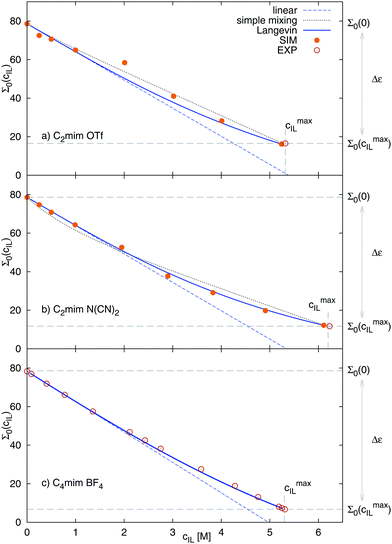 |
| | Fig. 5 Dielectric decrement of Σ0(cIL) at the zero frequency limit as a function of ionic liquid concentration of (a) [C2mim][OTf] (exp. Σ0(cmaxIL) from ref. 20), (b) [C2mim][N(CN)2] (exp. Σ0(cmaxIL) from ref. 68) and (c) [C4mim][BF4], where data was taken solely from ref. 70. The continuous line refers to the Langevin function of eqn (24), the dashed line to the respective linear fit of the initial slope, and the dotted line to simple mixing of εbulk, εhyd and Σ0,IL. The fit parameter εhyd was found to equal 76.5 for [C2mim][OTf], and 66.8 for [C2mim][N(CN)2]. | |
Table 3 Slopes αexcess and δ, obtained from the depression of the dielectric constant at cIL ≤ 1 M. Modified slope α′, obtained viaeqn (20). All values in [M−1]
| Ionic liquid |
ε
W(cIL) |
Σ
0(cIL) |
|
α′ |
α
excess
|
δ
|
α′ |
α
excess
|
δ
|
| [C2mim][OTf] |
17.6 |
24.3 |
−12.2 |
7.7 |
14.6 |
−7.3 |
| [C2mim][N(CN)2] |
16.5 |
22.2 |
−11.1 |
9.0 |
14.7 |
−7.4 |
| [C4mim][BF4]70 |
|
|
|
7.4 |
15.7 |
−7.9 |
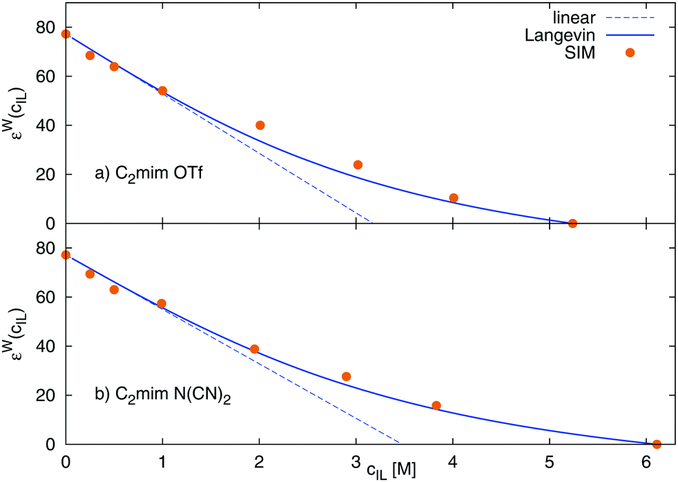
The Langevin functional dependency, eqn (23), can also be applied to the water contribution to the dielectric constant, εW, shown in Fig. 6, where a larger initial slope of 24 M−1 for [C2mim][OTf], and 22 M−1 for [C2mim][N(CN)2] is found. Thus, the water contribution εW changes to a larger extent with the ionic liquid concentration than the overall static dielectric constant Σ0.
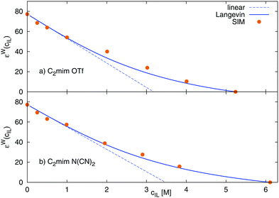 |
| | Fig. 6 Dielectric decrement of the water contribution εW as a function of ionic liquid concentration of (a) [C2mim][OTf] and (b) [C2mim][N(CN)2] The continuous line refers to the Langevin function of eqn (23), and the dashed line to the respective linear fit of the initial slope. | |
4.3 Static conductivity
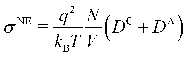
The static conductivity σ(0) obtained viaeqn (8) is listed in Table 4. For reasons of clarity, we write σ instead of σ(0) in the following, referring always to the zero-frequency limit of the conductivity. Table 4 also lists the diffusion coefficients Dx of cations, anions and water, as well as the resulting conductivity via the Nernst–Einstein equation| | 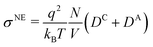 | (26) |
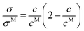
where q is the charge of the ion, N the number of ions and V the simulated volume. In general, σNE corresponds to the law of independent migration of ions, where the individual contributions are assumed to be additive and uncorrelated. The conductivity σ is related to σNEviaFor the studied systems, Δ is on average 0.25, and does not show a trend with the concentration of the ionic liquid. In general, a small Δ points to a small degree of collectivity. Thus, the interactions between cations and anions at all concentrations are weak to intermediate.
Table 4 Diffusion coefficients of anions, cations and water, as well as respective conductivity viaeqn (8) (σ) or via the Nernst–Einstein relation (σNE, Δ)
| IL |
c
IL [M] |
D
C [Å ps−1] |
D
A [Å ps−1] |
D
W [Å ps−1] |
σ [S m−1] |
σ
NE [S m−1] |
Δ
|
| C2mim OTf |
0.25 |
0.12 |
0.099 |
0.25 |
1.42 |
2.01 |
0.29 |
| 0.50 |
0.076 |
0.090 |
0.23 |
2.39 |
3.09 |
0.23 |
| 1.00 |
0.066 |
0.057 |
0.18 |
3.41 |
4.59 |
0.26 |
| 2.01 |
0.035 |
0.033 |
0.10 |
3.68 |
5.14 |
0.28 |
| 3.02 |
0.015 |
0.014 |
0.048 |
2.46 |
3.26 |
0.25 |
| 4.01 |
0.005 |
0.004 |
0.015 |
1.08 |
1.26 |
0.14 |
| 5.24 |
0.002 |
0.001 |
0.000 |
0.48 |
0.60 |
0.21 |
|
|
| C2mim N(CN)2 |
0.25 |
0.090 |
0.16 |
0.26 |
1.64 |
2.32 |
0.29 |
| 0.50 |
0.087 |
0.12 |
0.24 |
2.62 |
3.75 |
0.30 |
| 0.99 |
0.079 |
0.096 |
0.22 |
4.37 |
6.43 |
0.32 |
| 1.95 |
0.058 |
0.067 |
0.15 |
5.44 |
9.11 |
0.40 |
| 2.90 |
0.033 |
0.043 |
0.10 |
6.18 |
8.18 |
0.24 |
| 3.83 |
0.018 |
0.026 |
0.057 |
4.60 |
6.18 |
0.26 |
| 4.91 |
0.009 |
0.013 |
0.030 |
3.08 |
4.08 |
0.25 |
| 6.11 |
0.004 |
0.005 |
0.000 |
1.48 |
2.01 |
0.26 |
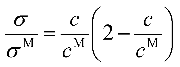
In 2010, Varela et al.4 reported a pseudolattice model of ionic transport in electrolyte solutions and ionic liquid mixtures, later completed by Cabeza and coworkers,2 which successfully described the static conductivity of ionic liquid mixtures leading to a parameter-free description of the normalized conductivity σ/σM with respect to the reduced concentration c/cM
| |  | (28) |
where
σM is the maximum value of the static conductivity occurring at the concentration
cM. This model, an evolution of the thermodynamic Bahe-Varela pseudolattice theory,
13,14 relies on a structural model of the ionic liquid mixture formed by a pseudolattice of cells-approximately corresponding to Adam–Gibbs rearranging regions
71 where ion cage and jump events take place, described among others by Araque
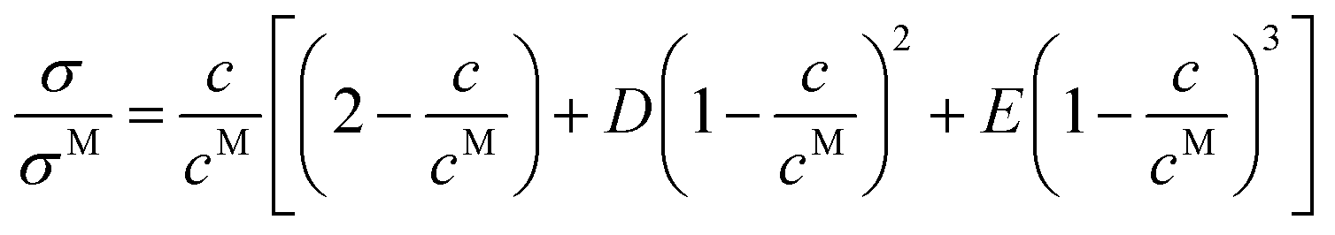
et al.72,73 by means of molecular dynamics simulations. Low mobility and high mobility cells are considered since, generally, liquid regions where charge depletion takes place are more easily rearrangeable (softer) and more mobile than regions where an enhancement of charge is registered. Moreover,
eqn (28) is recovered if one considers that the different cells are independent and ionic jumps uncorrelated (ideal level of theory), hence neglecting couplings between charge solutes and cosolvents which are, of course, very relevant at high concentrations. These interaction cause static and dynamical couplings essentially at two levels: (i) conditioning the way how cosolvent molecules mix with the ionic liquid (homogeneous or heterogeneous mixing), and (ii) correlated motion of charged species and solvent molecules, which gives rise to jumping frequencies depending on the type of cells from and to which hopping takes place. Although a detailed description of these complex phenomena demands the introduction of Bragg–Williams-like terms in the model, a simplified phenomenological description based on the instruction of additional terms in
eqn (28) was reported by Rilo
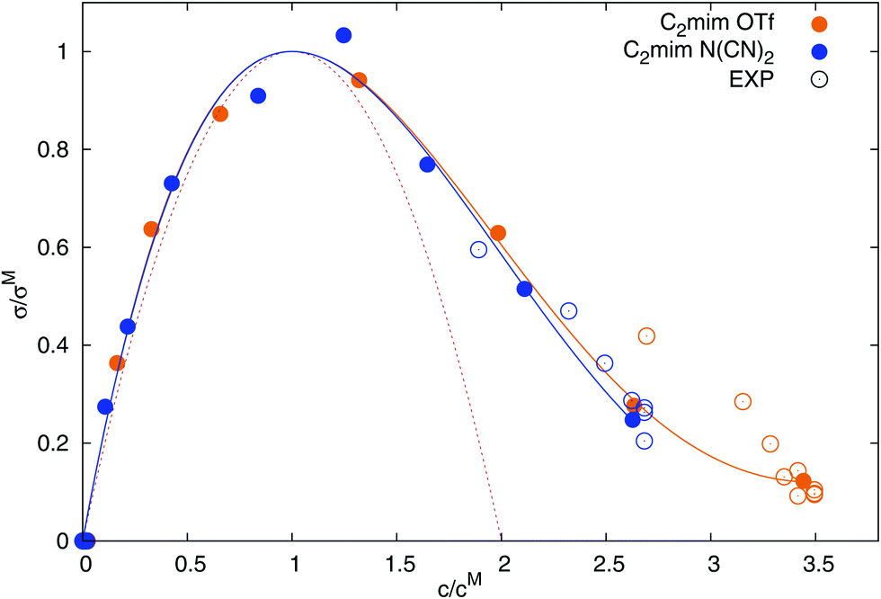
et al.2| |  | (29) |
where
D and
E are fitting parameters. The resulting universal curve of
eqn (28) is shown in red (dashed line) in
Fig. 7, and corresponds well to the computed conductivities at small to intermediate concentrations. The corrected universal curve of
eqn (29), continuous lines in
Fig. 7, describes
σ well at all concentrations. All parameters are given in
Table 5. We thus confirm the applicability of the universal conductivity parabola as reported by Cabeza and coworkers.
2,4 For the description of the experimental data
5,48,50–53,74,75 in
Fig. 7, the same
cM was used as for the computed conductivities in this study, but with a scaled
σM (scaling factor of 2.4 for [C
2mim][OTf], and 1.8 for [C
2mim][N(CN)
2]). The scaling of
σM is necessary since our simulations underestimate the experimental conductivity, although not as severely as previously published simulations.
19
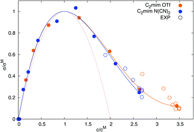 |
| | Fig. 7 Dependence of the normalized static conductivity on the reduced ionic liquid concentration. Experimental values from ref. 5, 48, 50–53, 74 and 75. The red dotted line corresponds to eqn (28) and the solid lines stem from eqn (29). | |
Table 5 Fit parameters of the conductivity hyperbola
| Ionic liquid |
c
M [M] |
σ
M [S m−1] |
D
|
E
|
| [C2mim][OTf] |
1.52 |
3.91 |
0.340 |
0.0378 |
| [C2mim][N(CN)2] |
2.33 |
5.81 |
0.325 |
0.0323 |
5 Conclusion
We computed the electric and dielectric properties at seven different concentrations of [C2mim][OTf]/water mixtures, and at eight different concentrations of [C2mim][N(CN)2]/water mixtures via polarizable MD simulation with scaled Lennard-Jones interactions. At low concentrations, the ionic liquid ions mainly arrange as direct contact ion pairs, small and charged clusters, or ion pairs mediated through one water molecule. At higher concentrations, ionic liquid domains form. The volume fraction of bulk water decreases exponentially with the ionic liquid concentration.
Consequently, we find that the water peak in the dielectric spectrum moves to lower frequencies, corresponding to slower processes, as more and more water molecules are affected (and retarded) by nearby ions. The dielectric spectra of the pure ionic liquids agree qualitatively with experimental spectra, and reproduce the peaks at ω ∼ 25 THz better than previously published spectra using polarizable force fields.19 The advantage is due to the more accurate description of the conductivity, which was underestimated by far in previous models. The scaling of the Lennard-Jones parameters employed in this work thus showed to improve the conductivity and dielectric constant of ionic liquids.
The static dielectric constant at the zero frequency limit diminished upon addition of ionic liquid to water, in agreement with the theory of the dielectric decrement. We find that the dielectric decrement can be described approximately using simple mixing rules (based on the volume fraction of the respective compounds) of the static permittivities of bulk water, pure ionic liquid and hydrated water. The effect of the ionic liquid ions on the dielectric constant of hydration water is small; we found a 3% decrease for water around [C2mim][OTf] and a 15% decrease for water around [C2mim][N(CN)2]. However, the volume fractions are only available computationally but not experimentally and a fitting parameter, namely the static dielectric constant of hydration water is required. We therefore instead adapted the Langevin-type functional dependence found by Gavish and Promislow33 for simple electrolyte solutions to fit the properties of ionic liquids. Our approach does not need any fit parameter, if the static dielectric constant of pure water, pure ionic liquid, and the depression of the dielectric constant at low concentration (i.e. the initial slope of the dielectric decrement) are known. The dielectric decrement of three different aqueous ionic liquid systems could be quantitatively described, one of them containing only experimental dielectric constants. The formula applies both for the overall static dielectric constant Σ0(0), and for the water rotational contribution εW(0). The rotational and translational contributions of the ions (εC(0), εA(0) and ϑ0(0)) do not show a Langevin-type behavior and feature a maximum at intermediate concentrations.
Finally, we calculated the conductivity of the ionic liquid/water mixtures at different concentrations. We found that the conductivities, although generally too low compared to experiment, conform to a universal behavior, namely that the normalized conductivity shows a parabolic dependence (with corrections at high concentrations) on the reduced concentration.2,4
Conflicts of interest
There are no conflicts to declare.
Acknowledgements
This work was funded by the Austrian Science Fund FWF in the context of Project No. P23494 and by the Cost Action CM 1206: “Exchange on ionic liquids”. Funding from Spanish Ministry of Economy and Competitiveness (Projects MAT2014-57943-C3-1-P and MAT2017-89239-C2-1-P) is gratefully acknowledged. Moreover, this work was funded by the Xunta de Galicia (AGRUP2015/11 and GRC ED431C 2016/001). E. H. is recipient of a DOC Fellowship of the Austrian Academy of Sciences at the Institute of Computational Biological Chemistry.
References
- M. J. Earle and K. R. Seddon, Pure Appl. Chem., 2000, 72, 1391 CrossRef.
- E. Rilo, J. Vila, S. García-Garabal, L. M. Varela and O. Cabeza, J. Phys. Chem. B, 2013, 117, 1411 CrossRef PubMed.
- J. Vila, P. Ginés, E. Rilo, O. Cabeza and L. M. Varela, Fluid Phase Equilib., 2006, 247, 32 CrossRef.
- L. M. Varela, J. Carrete, M. García, L. J. Gallego, M. Turmine, E. Rilo and O. Cabeza, Fluid Phase Equilib., 2010, 298, 280 CrossRef.
- P.-Y. Lin, A. N. Soriano, R. B. Leron and M.-H. Li, Exp. Therm. Fluid Sci., 2011, 35, 1107 CrossRef.
- P. Debye and E. Hückel, Phys. Z., 1923, 24, 185 Search PubMed.
- L. Onsager, Phys. Z., 1926, 27, 388 Search PubMed.
- L. Onsager and R. M. Fuoss, J. Phys. Chem., 1932, 36, 2689 CrossRef.
- L. Onsager and R. M. Fuoss, Proc. Natl. Acad. Sci. U. S. A., 1955, 41, 274 CrossRef.
- L. Onsager and R. M. Fuoss, J. Phys. Chem., 1957, 61, 668 CrossRef.
- L. Onsager and R. M. Fuoss, J. Phys. Chem., 1958, 62, 1339 CrossRef.
- R. M. Fuoss, J. Am. Chem. Soc., 1958, 80, 3163 CrossRef.
- L. W. Bahe, J. Phys. Chem., 1972, 76, 1062–1071 CrossRef.
- L. Varela, M. Garcia, F. Sarmiento, D. Attwood and V. Mosquera, J. Chem. Phys., 1997, 107, 6415–6419 CrossRef.
- R. Buchner and G. Hefter, Phys. Chem. Chem. Phys., 2009, 11, 8984 RSC.
-
C. J. F. Böttcher and P. Bordewijk, Theory of electric polarization, Elsevier, Amsterdam, 1978, vol. 1 Search PubMed.
-
F. Kremer and A. Schönhals, Broadband Dielectric Spectroscopy, Springer, Berlin, 2002 Search PubMed.
- C. Schröder and O. Steinhauser, J. Chem. Phys., 2009, 131, 114504 CrossRef PubMed.
- C. Schröder, T. Sonnleitner, R. Buchner and O. Steinhauser, Phys. Chem. Chem. Phys., 2011, 13, 12240 RSC.
- M.-M. Huang, Y. Jiang, P. Sasisanker, G. D. Driver and H. Weingärtner, J. Chem. Eng. Data, 2011, 56, 1494 CrossRef.
- G. H. Haggis, J. B. Hasted and T. J. Buchanan, J. Chem. Phys., 1952, 20, 1452 CrossRef.
- H. Looyenga, Physica, 1965, 31, 401 CrossRef.
- J. R. Birchak, L. G. Gardner, J. W. Hipp and J. M. Victor, Proc. IEEE, 1974, 62, 93 CrossRef.
-
C. J. F. Böttcher and P. Bordewijk, Theory of electric polarization, Elsevier, Amsterdam, 1978, vol. 2 Search PubMed.
- D. A. G. Bruggeman, Ann. Phys., 1935, 24, 636 CrossRef.
- P. N. Sen, C. Scala and M. H. Cohen, Geophysics, 1981, 46, 781 CrossRef.
- B. R. Pujari, B. Barik and B. Behera, Phys. Chem. Liq., 1998, 36, 105 CrossRef.
- C. Schröder, M. Sega, M. Schmollngruber, E. Gailberger, D. Braun and O. Steinhauser, J. Chem. Phys., 2014, 140, 204505 CrossRef PubMed.
- D. Ben-Yaakov, D. Andelman and R. Podgornik, J. Chem. Phys., 2011, 134, 074705 CrossRef PubMed.
- B. Maribo-Mogensen, G. M. Kontogeorgis and K. Thomsen, J. Phys. Chem. B, 2013, 117, 10523 CrossRef PubMed.
- F. Booth, J. Chem. Phys., 1951, 19, 391 CrossRef.
- R. L. Fulton, J. Chem. Phys., 2009, 130, 204503 CrossRef PubMed.
- N. Gavish and K. Promislow, Phys. Rev. E, 2016, 94, 012611 CrossRef PubMed.
- A. Levy, D. Andelman and H. Orland, Phys. Rev. Lett., 2012, 108, 227801 CrossRef PubMed.
- R. A. X. Persson, Phys. Chem. Chem. Phys., 2017, 19, 1982 RSC.
- C. Schröder, T. Rudas, G. Neumayr, S. Benkner and O. Steinhauser, J. Chem. Phys., 2007, 127, 234503 CrossRef PubMed.
- C. Schröder, J. Hunger, A. Stoppa, R. Buchner and O. Steinhauser, J. Chem. Phys., 2008, 129, 184501 CrossRef PubMed.
- C. Schröder, G. Neumayr and O. Steinhauser, J. Chem. Phys., 2009, 130, 194503 CrossRef PubMed.
- C. Schröder and O. Steinhauser, J. Chem. Phys., 2010, 132, 244109 CrossRef PubMed.
- M. Sega and C. Schröder, J. Phys. Chem. A, 2015, 119, 1539 CrossRef PubMed.
- G. Neumayr, C. Schröder and O. Steinhauser, J. Chem. Phys., 2009, 131, 174509 CrossRef PubMed.
- G. Lamoureux, A. D. MacKerell and B. Roux, J. Chem. Phys., 2003, 119, 5185 CrossRef.
- L. Huang and B. Roux, J. Chem. Theory Comput., 2013, 9, 3543 CrossRef PubMed.
- K. Vanommeslaeghe and A. D. MacKerell Jr., J. Chem. Inf. Model., 2012, 52, 3144 CrossRef PubMed.
- K. Vanommeslaeghe and A. D. MacKerell Jr., J. Chem. Inf. Model., 2012, 52, 3155 CrossRef PubMed.
- T. M. Becker, D. Dubbeldam, L.-C. Lin and T. J. H. Vlugt, J. Comput. Sci., 2016, 15, 86 CrossRef.
-
A. Kazakov, J. Magee, R. D. Chirico, E. Paulechka, V. Diky, C. D. Muzny, K. Kroenlein and M. Frenkel, NIST Standard Reference Database 147: NIST Ionic Liquids Database – (ILThermo), Version 2.0, http://ilthermo.boulder.nist.gov.
- C. Schreiner, S. Zugmann, R. Hartl and H. J. Gores, J. Chem. Eng. Data, 2010, 55, 1784 CrossRef.
- A. N. Soriano, B. T. Doma Jr. and M.-H. Li, J. Chem. Thermodyn., 2009, 41, 301 CrossRef.
- A. Stoppa, R. Buchner and G. Hefter, J. Mol. Liq., 2010, 153, 46 CrossRef.
- K. R. Harris and M. Kanakubo, J. Chem. Eng. Data, 2016, 61, 2399–2411 CrossRef.
- R. Aranowski, I. Chichowska-Kopczyńska, B. Dębski and P. Jasiński, J. Mol. Liq., 2016, 221, 541–546 CrossRef.
- M. Tsamba, S. Sarraute, M. Traikia and P. Husson, J. Chem. Eng. Data, 2014, 59, 1747–1754 CrossRef.
- G. Lamoureux and B. Roux, J. Chem. Phys., 2003, 119, 3025 CrossRef.
- S. Nosé, J. Chem. Phys., 1984, 81, 511 CrossRef.
- W. G. Hoover, Phys. Rev., 1985, A31, 1695 Search PubMed.
- C. Schröder, C. Wakai, H. Weingärtner and O. Steinhauser, J. Chem. Phys., 2007, 126, 084511 CrossRef PubMed.
- U. Kaatze, J. Solution Chem., 1997, 26, 1049 CrossRef.
- W. R. Tinga, W. A. G. Voss and D. F. Blossey, J. Appl. Phys., 1973, 44, 3897 CrossRef.
- A. H. Shivola, IEEE Trans. Geosci. Remote Sens., 1989, 27, 403 CrossRef.
- J. N. A. Canongia Lopes and A. A. H. Pádua, J. Phys. Chem. B, 2006, 110, 3330 CrossRef PubMed.
- W. Jiang, Y. Wang and G. A. Voth, J. Phys. Chem. B, 2007, 111, 4812 CrossRef PubMed.
- C. Schröder, J. Chem. Phys., 2011, 135, 024502 CrossRef PubMed.
- C. Schröder, Phys. Chem. Chem. Phys., 2012, 14, 3089 RSC.
- M. Eigen and K. Tamm, Z. Elektrochem., 1962, 66, 107–121 Search PubMed.
- D. A. Turton, J. Hunger, A. Stoppa, G. Hefter, A. Thoman, M. Walther, R. Buchner and K. Wynne, J. Am. Chem. Soc., 2009, 131, 11140 CrossRef PubMed.
- E. Heid, S. Harringer and C. Schröder, J. Chem. Phys., 2016, 145, 164506 CrossRef PubMed.
- J. Hunger, A. Stoppa, S. Schrödle, G. Hefter and R. Buchner, Chem. Phys. Chem., 2009, 10, 723 CrossRef PubMed.
- J. B. Hasted, D. M. Ritson and C. H. Collie, J. Chem. Phys., 1948, 16, 1 CrossRef.
- M. Koeberg, C.-C. Wu, D. Kim and M. Bonn, Chem. Phys. Lett., 2007, 439, 60 CrossRef.
- G. Adam and J. H. Gibbs, J. Chem. Phys., 1965, 43, 139–146 CrossRef.
- J. C. Araque, S. K. Yadav, M. Shadeck, M. Maroncelli and C. J. Margulis, J. Phys. Chem. B, 2015, 119, 7015–7029 CrossRef PubMed.
- J. C. Araque, J. J. Hettige and C. J. Margulis, J. Phys. Chem. B, 2015, 119, 12727–12740 CrossRef PubMed.
- Y.-H. Yu, A. N. Soriano and M.-H. Li, J. Chem. Thermodyn., 2009, 41, 103 CrossRef.
- P.-Y. Lin, A. N. Soriano, R. B. Leron and M.-H. Li, J. Chem. Thermodyn., 2010, 42, 994–998 CrossRef.
Footnote |
| † Electronic supplementary information (ESI) available: Force fields, fit parameters. See DOI: 10.1039/c8cp02111b |
|
| This journal is © the Owner Societies 2018 |
Click here to see how this site uses Cookies. View our privacy policy here. 
 Open Access Article
 This Open Access Article is licensed under a
  a,
Borja
Docampo-Álvarez
a,
Borja
Docampo-Álvarez


 , so that the dielectric constant drops to the known value ε(cmaxIL) of the pure ionic liquid at cmaxIL (instead of the artificial quantity εMS at cIL → ∞). Fig. 4 illustrates the necessity to renormalize the Langevin function using Lmax. The slope at small concentrations is then
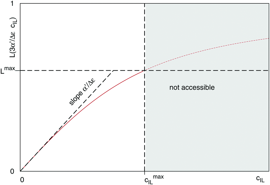
 . Since the concentration of ionic liquids cannot go beyond the concentration of the pure liquid, cmaxIL, the Langevin function varies between
 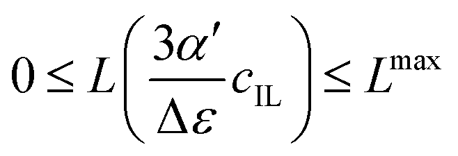 instead of
 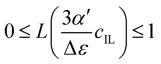 . Renormalization with Lmax resolves the issue.