Magnetism of NaFePO₄ and related polyanionic compounds

Abstract

Magnetic properties of maricite (m) and triphlyte (t) polymorphs of NaFePO₄ are investigated by combining ab initio density functional theory with a model Hamiltonian approach, where a realistic Hubbard-type model for magnetic Fe 3d states in NaFePO₄ is constructed entirely from first-principles calculations. For these purposes, we perform a comparative study based on the pseudopotential and linear muffin-tin orbital methods while tackling the problem of parasitic non-sphericity of the exchange–correlation potential. Upon calculating the model parameters, magnetic properties are studied by applying the mean-field Hartree–Fock approximation and the theory of superexchange interactions to extract the corresponding interatomic exchange parameters. Despite some differences, the two methods provide a consistent description of the magnetic properties of NaFePO₄. On the one hand, our calculations reproduce the correct magnetic ordering for t-NaFePO₄ allowing for magnetoelectric effect, and the theoretical values of Néel and Curie–Weiss temperatures are in fair agreement with reported experimental data. Furthermore, we investigate the effect of chemical pressure on magnetic properties by substituting Na with Li and, in turn, we explain how a noncollinear magnetic alignment induced by an external magnetic field leads to magnetoelectric effect in NaFePO₄ and other transition-metal phosphates. However, the origin of a magnetic superstructure with q = (1/2, 0, 1/2) observed experimentally in m-NaFePO₄ remains puzzling. Instead, we predict that competing exchange interactions can lead to the formation of magnetic superstructures along the shortest orthorhombic c axis of m-NaFePO₄, similar to multiferroic manganites.

---

1 Introduction

Polyanionic compounds are based on molecular frameworks that combine tetrahedron anion units (XO₄)ⁿ⁻ (with X = S, P, Si, As, Mo, or W), or their derivatives (X_mO_3m+1)ⁿ⁻, and MO_x polyhedra (with M = transition metals). From a technological viewpoint, this class of materials is interesting due to their attractive electrochemical properties for high energy density cathodes in rechargeable batteries.^1,2 In particular, their broad structural diversity, strong inductive effect of polyanions, and minimal structural rearrangement and volume change during alkali metal ion insertion create a fertile playground to design suitable operating voltage materials with outstanding cycling performance. This has triggered a surge of research among the battery community in recent years, which led to the discovery of a number of new polyanionic compounds.^3,4

Apart from their good electrochemical properties, other facets of potential interest in polyanionic compounds are however less explored. One prominent example is magnetism.³ Indeed, 3d-metal-based polyanionic compounds show unusual magnetic properties that can give rise to many appealing phenomena such as magnetoelectricity^5–12 and even multiferroicity.¹³ The origin of such a rich magnetic behavior is a consequence of the combination of M–O–M super-exchange and M–O–X–O–M super-super-exchange interactions in these materials, which can induce the emergence of complex magnetic structures.

In this work, we focus on the magnetic properties of sodium iron phosphate (NaFePO₄), the sodium counterpart of lithium iron phosphate (LiFePO₄). LiFePO₄ is one of the most studied cathode materials for today's Li-ion batteries.¹⁴ Yet the high abundance, environment-friendly nature, and low cost of sodium have made the research in Na-based electrode materials a topic of high interest,^15–22 with an ongoing flurry of activity in NaFePO₄ (see, e.g., Fang et al.²³). NaFePO₄ crystallizes in two different polymorphic forms: triphlyte (t) and maricite (m). m-NaFePO₄ is the thermodynamically stable phase and shows many similarities with orthorhombically distorted transition-metal (TM) perovskite oxides,^24,25 whereas t-NaFePO₄ is isostructural to LiFePO₄. Avdeev et al. studied both polymorphs by means of neutron powder diffraction (NPD) experiments and magnetic susceptibility measurements.²⁶ The magnetic properties of NaFePO₄ are indeed very interesting and rather complex. According to NPD measurements,²⁶ t-NaFePO₄ forms the same simple antiferromagnetic (AFM) order as LiFePO₄,²⁷ which is expected to reveal magnetoelectric effect.⁸ On the other hand, m-NaFePO₄ tends to form a magnetic superstructure with the propagation vector q = (1/2, 0, 1/2),²⁶ which implies the existence of competing magnetic interactions in the system. The situation is particularly interesting in the light that there are many examples of orthorhombic manganites, where such competition also results in the formation of magnetic superstructures that break inversion symmetry and give rise to the multiferroic behavior.^28–30 The magnetic transition temperature, T_N, is also very different, 50 K in t-NaFePO₄ and only 13 K in m-NaFePO₄, while the Curie–Weiss temperature (θ) is comparable in both phases and is about −80 K. The first theoretical attempt to study the magnetic properties of NaFePO₄ was undertaken by Kim et al. using brute force total-energy calculations based on density functional theory (DFT) with a semi-phenomenological on-site Coulomb repulsion U.³¹ They concluded that while the magnetic structure of t-NaFePO₄ can be understood by the spin exchange alone, the one of m-NaFePO₄ apparently involves additional mechanisms, such as magnetic anisotropy.

In this work, we aim at understanding the magnetic properties of NaFePO₄ by means of effective model Hamiltonians constructed from first-principles electronic structure calculations in the Wannier basis for the set of magnetically active target Fe 3d bands. This approach treats the Coulomb interaction problem more rigorously than brute force total-energy calculations. Moreover, the model can provide deep insight into the microscopic origin of the magnetic interactions in polyanionic compounds and help to analyze the results of brute force calculations. Furthermore, we present a comparative study considering two different numerical implementations of the Wannier functions technique; one based on the pseudopotential method and the other on the minimal basis set linear muffin-tin orbital method.

The paper is organized as follows. In Section 2, we outline the details of the electronic structure calculations, as well as the methods used to construct and solve model Hamiltonians. Then, in Section 3, we present our main results for interatomic exchange interactions and relative stability of different magnetic states. We also consider the effect of chemical pressure on the magnetic properties and magnetoelectric effect in triphlytes. Finally, the results are recapitulated and summarized in Section 4.

2 Method

2.1 Crystal structure

Both t- and m-NaFePO₄ crystallize in the orthorhombic structure with the space group Pnma (No. 62 in the International Tables). Both polymorphs contain four formula units in the primitive cell, where all Fe sites are equivalent (i.e., can be transformed to each other by the symmetry operations of the Pnma space group), as shown in Fig. 1. The structure of t-NaFePO₄ involves corner-sharing FeO₆ distorted octahedra and PO₄ tetrahedra that share edges with first-neighbor Fe-sites and corners with the rest of the surrounding octahedra, as shown in Fig. 1(a) and (b). The Fe sites are located off the inversion centers, which are occupied by Na atoms. In the m-phase, the distorted FeO₆ octahedra share edges with equivalent FeO₆ units, forming short Fe–O–Fe contacts in a chain-like fashion. The PO₄ tetrahedra share corners with FeO₆ units, ‘binding’ the chains together as shown in Fig. 1(c) and (d).

Fig. 1 ab and ac projections of the crystal structure of t- (a and b) and m-NaFePO₄ (c and d). Na, P, Fe and O atoms are shown with yellow, gray, brown and red spheres, respectively.

2.2 Electronic structure in GGA

In order to obtain the electronic structure of t- and m-NaFePO₄ we performed DFT calculations using the generalized gradient approximation (GGA) with the PBE exchange–correlation functional.³² We used the Quantum-ESPRESSO (QE) (version 6.1) package, where we replaced the core electrons with norm-conserving pseudopotentials (NCPPs) and treated explicitly the Na (3s¹), Fe (3d⁶4s²), P (3s²3p³), and O (2s²2p⁴) electrons as valence states. Their wave functions were expanded in plane waves with a kinetic energy cutoff of 100 Ry and a charge density cutoff of 400 Ry. A tight energy convergence criteria of 10⁻⁸ Ry was used with a k-point sampling of 4 × 8 × 10 (6 × 8 × 10) for the t-(m-) NaFePO₄. All calculations have been performed with the experimental structural parameters.²⁶

The calculated GGA density of states (DOS) for t- and m-NaFePO₄ is shown in Fig. 2. Typically, the character of insulating TM oxides changes along the Ti–Cu³³ series. Early oxides of Ti–Cr are normally regarded as Mott insulators, while late oxides exhibit a strong charge transfer character because the TM 3d states strongly hybridize with the O 2p states and, therefore, O atoms also contribute to the low-energy properties. While the properties of Mott insulators can be described by a conventional Hubbard-type model, charge transfer insulators require further model refinements in order to include the O 2p states explicitly. Yet, orthophosphates are a notorious exception to this general situation because PO₄³⁻ species have a clear molecular character which leads to additional band splittings into bonding states (mainly formed by the O 2p orbitals) and antibonding states (formed by the P 3p orbitals). As a consequence, the bonding O 2p states are additionally shifted to the low-energy region, which increases their separation from the Fe 3d states. Thus, the Fe 3d states form a narrow band located near the Fermi level, which is very well separated from both the O 2p bands (from below) and the P 3p bands (from above), as shown in Fig. 2. This makes the description of these materials particularly suitable for applying a Hubbard model. In the following, we will construct such a model by employing the Wannier functions method.^34,35 Then, we will solve this model in the mean-field Hartree–Fock (HF) approximation and calculate all relevant parameters of interatomic exchange interactions. Since the degeneracy of the ground state of NaFePO₄ is lifted by the lattice distortion, the ground-state wavefunction can be described by a single Slater determinant, which justifies the use of the HF approximation.

Fig. 2 Total and partial PBE DOS for t- and m-NaFePO₄. The shaded blue area shows contributions from the Fe 3d states. The Fermi level is at zero energy.

2.3 Construction and solution of the Hubbard model

To describe magnetically active Fe 3d states in t- and m-NaFePO₄, we employed the Wannier functions technique^34,35 as an effective basis to construct a Hubbard-type model:where ĉ^†_iaσ (ĉ_iaσ) are the creation (annihilation) operator acting at lattice points i, j on a Wannier orbital w_iaσ, σ(σ′) = ↑ or ↓ is the projection of spin, and the five Wannier functions at each Fe site are a, b, c, and d. In QE calculations, in order to obtain the Wannier functions for the 20 Fe 3d bands, we employ the technique of maximal localization.³⁴ The resulting Wannier functions are indeed well localized at Fe sites, as shown in Fig. 3 for a = 1–5. The individual spreads, 〈r²〉_a, are 1.66, 1.04, 1.14, 1.21, and 1.47 Ų for t-NaFePO₄, and 1.62, 1.15, 1.01, 1.84, and 1.22 Ų for m-NaFePO₄. In addition, the Wannier representation of the PBE band-structure [Fig. 3(a) and (b)] is nearly perfect for the 3d bands, and the d-orbital character of the Wannier functions w_ia(r) is visually apparent [Fig. 3(c) and (d)].

Fig. 3 (a) PBE (turquoise solid lines) and (b) Wannier interpolated (blue dashed lines) band structures for the low-energy Fe 3d states as obtained for t- and m-NaFePO₄, respectively. The corresponding real-space Wannier functions centered at Fe sites are shown for t-NaFePO₄ (c) and m-NaFePO₄ (d). Notations of the high symmetry points of the Brillouin zone are taken from ref. 36.

Then, the transfer integrals and the crystal-field splitting, which are incorporated in [t^ij_ab], are evaluated as the matrix elements of the GGA Hamiltonian in the Wannier basis, as will be discussed below in detail. The screened Coulomb interactions are evaluated by using constrained random-phase approximation (cRPA).³⁷ in eqn (1) are the matrix elements of spin–orbit (SO) coupling, which are also derived from the GGA Hamiltonian. In addition to the QE approach, we performed similar calculations by using the linear muffin-tin orbital (LMTO) method.^38,39 The details of the model Hamiltonian construction in this case can be found in ref. 35.

In order to evaluate the one-electron part of the model Hamiltonian, t̂ = [t^ij_ab] in eqn (1), we considered different computational schemes.

Scheme 1 (s1): The one-electron part is evaluated ‘as is’ and identified with the matrix elements of the GGA Hamiltonian calculated in the Wannier basis. In this case, t̂ already takes into account non-sphericity of the Coulomb and exchange–correlation potentials. Therefore, in order to avoid double counting, we have to remove them when dealing with Coulomb and exchange interactions in the Hubbard model. For these purposes, we employed the spherical parametrization of the screened Coulomb interactions obtained from cRPA, Û = [U_abcd], with the following values for the on-site Coulomb repulsion U = F⁰, intra-atomic exchange interaction J = (F² + F⁴)/14, and the ‘nonsphericity’ B = (9F² − 5F⁴)/441 (F⁰, F², and F⁴ being the screened radial Slater's integrals), which fully specify Û in the atomic spherical environment. Then, in the HF calculations, we set U_aabb = U for any a and b, and U_abba = J for a ≠ b. This guarantees that the Coulomb part of the HF potential is spherical and the exchange part, besides intra-atomic Hund's rule, is responsible for the appearance of a discontinuity term, which is proportional to U–J and missing in ordinary GGA. Other effects are included in t̂ and described at GGA level. Thus, the idea is similar to DFT+U.⁴⁰ The logic here is the following: the electron configuration d⁶ of the Fe²⁺ ions in NaFePO₄ is essentially non-spherical. According to the fundamental Hohenberg–Kohn theorem,⁴¹ this non-sphericity should be properly described by DFT, and GGA, as one of its possible approximations, should capture this effect in a certain form. The discontinuity of the exchange potential in the HF method does not affect the total energies of isolated ions and leads only to rearrangement of single-particle levels between occupied and empty states.⁴² However, in solids, where these levels become connected by transfer integrals, the discontinuity already contributes to the total energy and other ground-state properties, as is clearly seen, for instance, in the theory of superexchange (SE) interactions.⁴³

Scheme 2 (s2): We additionally subtract from t̂ the matrix elements of the GGA exchange–correlation potential in the Wannier basis, 〈w_i|V_xc|w_j〉. The basic idea behind is to fully replace the exchange–correlation interactions in GGA by the ones obtained for the Hubbard model. Thus, in the HF calculations, we use the full matrix Û = [U_abcd], obtained in cRPA without additional approximations for the exchange part of the HF potential. At the same time, non-sphericity of the Coulomb potential is treated at GGA level and already included in t̂. Therefore, for the Coulomb potential in the HF method, we keep using the spherical form of Û, which is described by a single parameter, U_aabb = U. Moreover, we consider two approximations. In the first approximation, we subtract from t̂ only site-diagonal matrix elements of the exchange–correlation potential, 〈w_i|V_xc|w_i〉. The logic is that since the Hubbard model (1) includes the on-site interactions, only the on-site interactions should be subtracted from GGA, assuming that other (intersite) interactions are described reasonably well at the GGA level. In the second approximation, we subtract both site-diagonal and intersite matrix elements, 〈w_i|V_xc|w_j〉.

Scheme 3 (s3): This scheme is based on the LMTO method.³⁵ The additional atomic-spheres approximation (ASA) in the LMTO method leads to some limitations for treating the electronic structure of NaFePO₄. In our calculations, we tried to choose the atomic spheres in LMTO so as to reproduce the electronic structure of the more accurate QE calculations. Nevertheless, the good aspect of the LMTO method is that it provides another possibility for elimination of non-spherical on-site Coulomb and exchange–correlation interactions in GGA: in ASA, all these interactions are spherically averaged inside the atomic spheres. Therefore, we do not need to worry about double counting of this non-shpericity, so all non-sphericity arises from the screened Coulomb and exchange interactions in the Hubbard model. In ASA, one should only include the additional correction due to non-sphericity of intersite Madelung potential.³⁵ As somewhat technical aspect, we had to use additional approximations in the process of cRPA calculations in the LMTO basis.³⁵ Namely, instead of constructing proper Wannier functions, we used pseudo-atomic LMTO basis to calculate Û. Therefore, since the atomic orbitals are more localized than the Wannier functions, the effective Coulomb interaction is a bit larger compared to full-scale QE cRPA calculations.

The corresponding crystal-field splitting obtained from the diagonalization of the site-diagonal part of t̂ is displayed in Fig. 4. A key parameter here is the energy separation of the crystal-field orbital 1, populated by the minority-spin electron, from the rest of the orbitals. For instance, this parameter controls the strength of the spin–orbit coupling effects and typically competes with the crystal-field splitting. In LMTO (s3) and QE (s1, without any corrections), the splitting between the levels 1 and 2 is of the order of 100 meV. However, subtraction of 〈w_i|V_xc|w_j〉 in s2 additionally splits off the orbital 1. The shape of the orbital 1 is also important. Its effect will be considered latter, separately for m- and t-NaFePO₄.

Fig. 4 Crystal-field splitting as obtained from QE with (s2) and without (s1) subtraction of the matrix elements of the GGA exchange–correlation potential, and LMTO method (s3) for the Fe 3d states of t- and m-NaFePO₄.

Having constructed and solved the effective model (1) by means of the mean-field HF approximation, one can calculate the one-electron (retarded) Green functions, and evaluate parameters of isotropic exchange interactions by using the local force theorem and considering perturbation theory to second order in infinitesimal spin rotations.⁴⁴ The corresponding expression is given by:

where is the difference of the HF potentials obtained for the majority (↑) and minority (↓) spin states, and Tr_L is the trace over orbital indices. The expression corresponds to the local mapping (which is valid only in a particular magnetic equilibrium state) of the total energies onto the spin model of the formwhere e_i is the direction of spin at site i. Similar expression can be derived for Dzyaloshinskii–Moriya (DM) interactions (corresponding to the energy change d_ij[e_i × e_j] in each magnetic bond) and higher-order anisotropic interactions, by considering perturbation theory with respect to spin–orbit coupling.^45,46

3 Results and discussions

3.1 m-NaFePO₄

We start our analysis with m-NaFePO₄, which is a somewhat easier example from the computational point of view. Particularly, since the Fe ions are located at the inversion centers and there are no additional complications related to the parity violation, we are able to implement all three schemes s1–s3 described above, including relatively heavy and time consuming cRPA calculations of the screened Coulomb interactions in the QE method.

Fig. 5 shows the parameters of the effective Coulomb and exchange interactions obtained in cRPA. As expected, the effective Coulomb repulsion calculated with the LMTO method is larger than the one obtained with QE. For instance, the parametrization in terms of U, J, and B (see Section 2) yields U = 3.7 and 2.9 eV for LMTO and QE, respectively. This is understandable, because the effective U in LMTO is evaluated within the basis of pseudo-atomic 3d orbitals, which are more localized than the proper Wannier orbitals used in the QE method. In all other respects, the behavior of matrix elements of Û is rather similar between the two methods, and the parameters J and B are close for both QE and LMTO methods: J = 0.9 eV and B = 0.1.

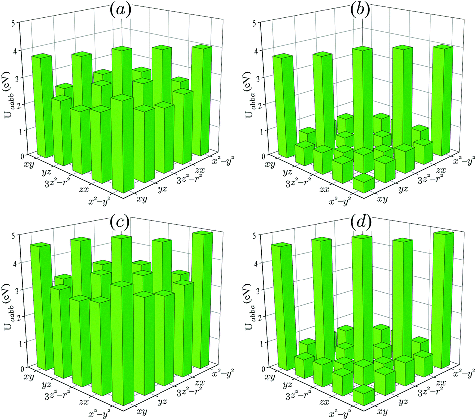Fig. 5 Matrix elements of Coulomb (a and c) and exchange (b and d) interactions for m-NaFePO₄ as obtained in the framework of cRPA in QE (a and b) and LMTO (c and d) calculations.

The behavior of transfer integrals can be illustrated by considering SE interactions, which are directly related to t̂_ij. The corresponding expression is given by:⁴⁷

where the last term stands for the AFM coupling describing the interaction of all majority- and minority-spin orbitals at the neighboring Fe sites, and the first two terms describe the FM coupling, which is caused by the population of the crystal-field orbital 1 by the minority-spin electron (and, in principle, depends on the orbital ordering – the shape of the populated orbital). In this expression, it is assumed that the transfer integrals t^ab_ij are in the crystal-field representation, which diagonalizes the site-diagonal part of t̂ and ε_a are the corresponding crystal-field orbitals. The crystal-field orbitals populated by the minority-spin electrons are displayed in Fig. 6 and the corresponding SE interactions are shown in Fig. 7. The sizeable interatomic exchange interactions spread up to the 5th coordination sphere. Other interactions are negligible in all of the schemes considered. This tendency is related to the behavior of transfer integrals, which are similar in all schemes. As expected, the largest interaction occurs between nearest neighbors. Moreover, the schemes s2 and s3 produce very similar results: in both cases, the strong AFM contributions are partly compensated by weaker FM ones. Thus, the total interactions remain AFM. The total interactions, as well as the partial contributions are practically the same in s2 and s3. This is somewhat surprising because the orbital ordering obtained in these two methods is quite different (Fig. 6). Nevertheless, to some extent, the effect of the orbital ordering is compensated by the transfer integrals, which for such low-symmetry systems mix all five types of orbitals. Therefore, different orbital orderings can produce similar exchange parameters. The SE interactions obtained in QE (without any corrections) are clearly different: in this case the AFM contribution is fully compensated by the FM one, resulting in a small FM coupling between nearest neighbors. However, to some extent, the discrepancy between s1 and s2 and s3 schemes is corrected by taking the full matrix of Coulomb interactions (and, if necessary, by applying appropriate corrections to it, as explained in Section 2) to calculate exchange interactions based on the local force theorem in the full scale HF calculations without SE approximation: in this case, the results of s1, s2, and s3 are more consistent with each other and in all three cases the nearest-neighbor coupling is found to be AFM (see Table 1).

Fig. 6 Orbital ordering (the electron density of occupied minority-spin orbital) in m-NaFePO₄ as obtained in (a) LMTO calculations, (b) QE calculations, and (c) QE calculations after subtraction of the GGA exchange–correlation potential.

Fig. 7 (a) Distance dependence of SE interactions as obtained in LMTO (s3) and QE calculations with (s2) and without (s1) subtraction of site-diagonal matrix elements of the GGA exchange–correlation potential. (b) Results obtained in the QE calculations after subtraction of both site-diagonal and off-diagonal matrix elements of the GGA exchange–correlation potential (s2). The FM and AFM contributions are shown by open red and cyan symbols, respectively, and the total contributions are shown by filled symbols. The symbols denote the type of interactions (see Fig. 6 for the notation of atomic positions).

Table 1 Interatomic exchange interactions (in meV) and corresponding Curie–Weiss temperature (in K) in m-NaFePO₄ (in meV) as obtained in LMTO (s3) and QE calculations with (s2) and without (s1) subtraction of site-diagonal matrix elements of the GGA exchange–correlation potential. The positions of atomic sites are defined in Fig. 6. The results of the simplified superexchange theory are denoted as ‘SE’, and the results obtained by using the local force theorem are denoted as ‘LF’

Method	J 12	J 33′	J 13	J 34′	J 14	J 14′	θ
s1, SE	0.02	−0.05	−0.39	−1.30	−1.61	−0.12	−80.4
s1, LF	−1.20	−0.08	−0.38	−1.27	−1.55	−0.13	−91.1
s2, SE	−3.19	−0.11	−0.11	−0.07	−1.32	−0.13	−76.5
s2, LF	−2.19	−0.12	−0.30	−0.72	−1.54	−0.17	−87.1
s3, SE	−3.54	−0.07	−0.17	−0.66	−0.95	−0.12	−86.5
s3, LF	−3.07	−0.06	−0.18	−0.67	−0.97	−0.12	−87.1

---

Finally, we note that the superexchange interactions obtained with the s2 scheme, after subtraction of both site-diagonal and off-diagonal elements of the GGA exchange–correlation potential, are strongly overestimated (Fig. 7b): the off-diagonal elements 〈w_i|V_xc|w_j〉 appear to be large and change the values of the transfer integrals. Thus, the construction of the model parameters in the scheme s2 is clearly unphysical: if one tries to correct GGA by adding only on-site electron–electron interactions, it is reasonable to subtract only the local (or site-diagonal) part of 〈w_i|V_xc|w_j〉.

Using the obtained parameters of exchange interactions, one can easily evaluate the Curie–Weiss temperature as . Depending on the computational scheme (s1–s3) and method to calculate the exchange parameters (SE versus the local force theorem), θ varies from −77 to −91 K (Table 1), being in fair agreement with the experimental value of −83 K reported by Avdeev et al.²⁶

The next important questions is how consistent the obtained parameters are with the experimental magnetic structure of m-NaFePO₄. Since the m-phase has the same symmetry as perovskite TM oxides, we can follow the same strategy as for the perovskites and, as the first step, compare the energies of FM, A-type AFM (the FM ac layers are antiferromagnetically coupled along b), C-type AFM (FM chains propagating along b and antiferromagnetically coupled in the ac plane), and G-type AFM (AFM coupling between nearest neighbors in all three directions) states. We have found that the A and C states are close in energy, and considerably lower than the FM and G states. The energy difference between C and A states varies from 8 meV per NaFePO₄ in the s3 scheme till 6 meV per NaFePO₄ in the s1 scheme. The A state is stabilized due to the AFM coupling J₁₂. The C state arises due to a joint effect of several long-range interactions (e.g., J₁₃ and J₁₄ in Table 1) that compete with J₁₂ and tend to make the coupling in the b chains ferromagnetic. The formation of the FM chains in the second case is consistent with the experimental data.²⁶ However, NPD measurements reveal a more complex magnetic structure, which is described by the propagation vector q = (1/2, 0, 1/2) and corresponds to the AFM coupling between chains separated by the translations along a and c.²⁶ In order to explore such possibility, we investigate the stability of the A and C states with respect to the incommensurate spin-wave excitations. Namely, we search for the eigenvalues ω_α of the 4 × 4 matrix , where the dimensionality corresponds to the number of magnetic sublattices in the unit cell, J̃_ij = ±J_ij for the ferromagnetically (+) and antiferromagnetically (−) coupled bonds, J̃_{[small script l][small script l]′}(q) is the Fourier image of J̃_ij between sublattices [small script l] and [small script l]′, and . If all ω_α(q) are positive, the magnetic state is stable. If some of them are negative, the state is unstable for given q. The results are shown in Fig. 8, using parameters obtained in the SE theory for the s1 scheme (other schemes provide qualitatively a similar picture). One can see that for the calculated value of U the A state is stable (all ω's are positive), while for the C phase some of the ω's are negative, even for q = 0. Thus, the magnetic ground state is expected to be of the A type. This is clearly inconsistent with the experimental data. To some extent, the problem can be resolved by decreasing the value of U, which increases the weight of the FM contributions [mainly the first term in eqn (4)] to J₁₂ and eventually makes this coupling ferromagnetic. For instance, the SE interaction J^SE₁₂ in the s1 scheme gradually increases from 0.01 meV to 4.58 meV when the Coulomb repulsion U changes from 2.94 eV to 1.47 eV. In reality, the underestimation of the FM contributions to the exchange coupling may be related to the lack of direct interatomic interactions in the considered Hubbard model, eqn (1),⁴⁸ which is mimicked by the change of the value of U in the expression for the SE interactions eqn (4). Anyway, for U* ≈ 0.5U (U being the calculated value) the A state becomes unstable for q = 0. Instead, the C state is stabilized. Furthermore, the minimal ω_α(q*) is obtained for q* ≈ (0, 0, 0.36), which is close to the Z-point in Fig. 8. Thus, one could expect the formation of the incommensurate magnetic ground state. For U* ≈ 0.5U, both A and C states are also unstable for the experimental q = (1/2, 0, 1/2) (the U-point in Fig. 8). However, according to the spin-wave analysis, the energy of this state is expected to be higher than that of the incommensurate state corresponding to q*. It is true that the energy difference between q* and U points of the Brillouin zone is small (about 1 meV). However, it is also true that the spin-wave dispersion along the Z–U direction is practically flat, meaning that there are no magnetic interactions along the a axis, which would stabilize the experimental q = (1/2, 0, 1/2) superstructure. This seems to be reasonable taking into account that a is the largest, while c is the shortest lattice parameter in m-NaFePO₄ (a/b = 1.310 and a/c = 1.782). Therefore, it is fair to expect the existence of strong magnetic interactions which would lead to the formation of magnetic superstructures along the c axis, but not along the a axis. Finally, we note that if the magnetic ground state of m-NaFePO₄ was indeed incommensurate with q* ≈ (0, 0, 0.36), this phase would be multiferroic, similar to the perovskite manganites with the same crystal and magnetic structures.^28–30 It would be interesting to explore this possibility experimentally.

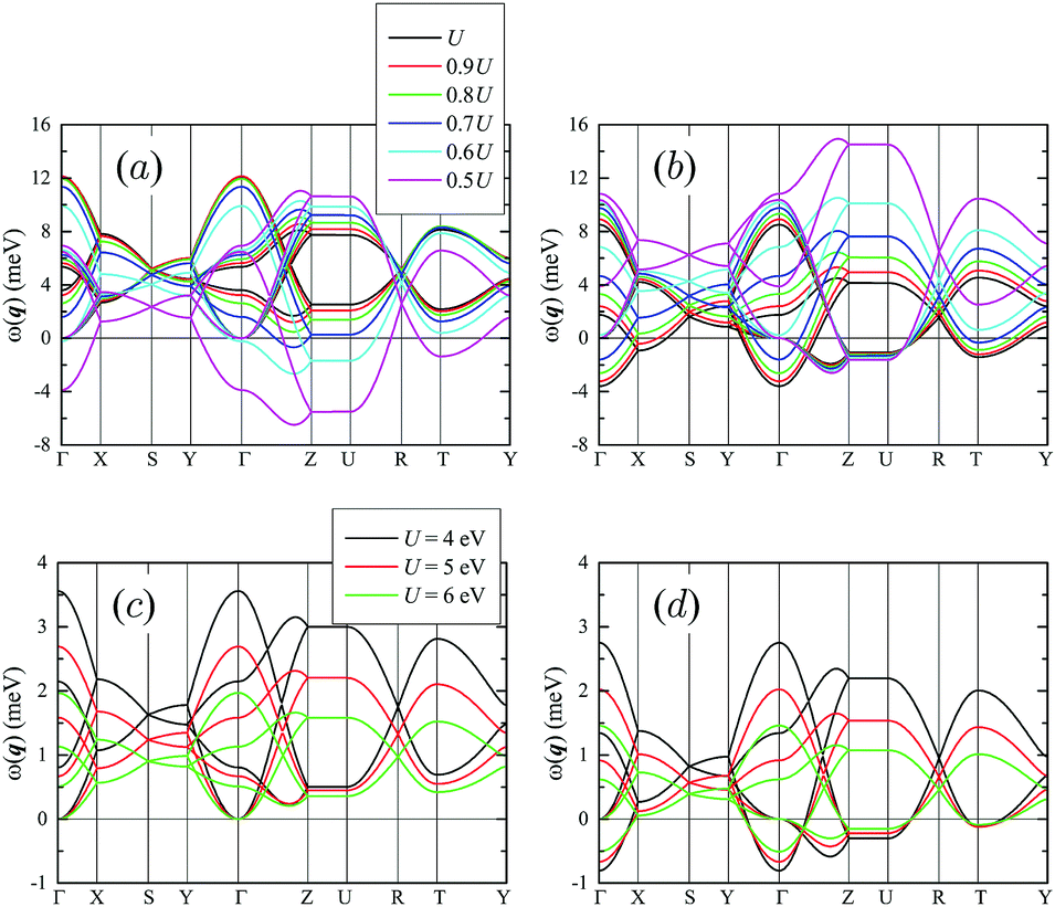Fig. 8 Spin-wave dispersion in the A- (a and c) and C-type (b and d) AFM state of m-NaFePO₄. (a and b) Obtained by using parameters of the SE interactions and scaling the value of the Coulomb repulsion from U = 2.94 eV to 0.5U = 1.47 eV. (c) and (d) were obtained by using parameters reported in Table 2 of ref. 31. The notations of the high symmetry points of the Brillouin zone are taken from ref. 36.

Regarding this apparent disagreement with the NPD data,²⁶ we would like to note that the parameters of interatomic exchange interactions for m-NaFePO₄ were also derived in ref. 31 by mapping the total energies, obtained for different magnetic structures in the DFT+U approach, onto the spin model of eqn (3). This procedure is different from the one used in this work. On the one hand, it takes into account the contributions of the oxygen band, which may be important. On the other hand, it suffers from ambiguities related to the choice of parameters and details of implementation of the DFT+U approach. Nevertheless, the main conclusion is similar to ours: if we use the exchange parameters reported in ref. 31 and evaluate ω_α, we readily obtain that the magnetic ground state is also A and there is no sign of instability towards a magnetic superstructure with q = (1/2, 0, 1/2). The relativistic SO interaction can lead to the canting of spins, similar to other perovskite TM oxides, crystallizing in the centrosymmetric Pnma structure.^35,45 However, the SO interaction alone cannot lead to the formation of superstructures. Thus, the microscopic origin of the q = (1/2, 0, 1/2) order, reported experimentally, is still puzzling.

3.2 t-NaFePO₄

Since the cRPA calculations of the screened Coulomb interactions in QE are very time consuming, for the t-phase of NaFePO₄ we consider only two schemes: s1, where we use the averaged values of Coulomb and exchange interactions obtained for the m-phase, and s3 (LMTO). Indeed, the averaged cRPA parameters of the effective Coulomb and exchange interactions obtained in the LMTO method, U = 3.5 eV, J = 0.9 eV, and B = 0.1 eV, are very close to those of the m-phase. Therefore, we expect similar tendency to hold in the QE calculations.

Without SO interaction, there are four possible collinear arrangements of the Fe spins in the primitive cell: ↑↑↑↑ (F), ↑↓↓↑ (A1), ↑↓↑↓ (A2), and ↑↑↓↓ (A3), where the arrows indicate the directions of spins at sites 1–4 (see Fig. 1). Amongst them, F and A3 contain spacial inversion Î as it is, while in A1 and A2 Î is combined with time reversal T̂. Thus, the latter two magnetic phases allow for magnetoelectric effect, which will be discussed in more detail in Section 3.4. The magnetic ground state is A1, in agreement with experiments.²⁶ In the HF approximation, the energy difference between F, A2, and A3 (on the one hand) and A1 (on the other hand) is 16.5 (26.0), 12.6 (22.7), and 2.1 (2.0) meV per NaFePO₄ in s1 (s3), respectively.

The interatomic exchange interactions obtained by using different techniques are summarized in Table 2. Like in m-NaFePO₄, we find a consistent description for J_ij, even despite a substantial change of the orbital ordering between the s1 and s3 schemes (Fig. 9).

Table 2 Interatomic exchange interactions (in meV) and corresponding Curie–Weiss and Néel temperatures (in K) in t-NaFePO₄ as obtained from LMTO (s3) and QE calculations without subtraction of site-diagonal matrix elements of the GGA exchange–correlation potential (s1). The positions of atomic sites are explained in Fig. 6. The results of the simplified superexchange theory are denoted as ‘SE’, and the results obtained by using the local force theorem are denoted as ‘LF’

Method	J 13	J 11′	J 12	J 1′4	J 14	J 1′1′′	θ	T N
s1, SE	−3.62	0.14	−1.66	−0.57	0.09	−2.16	−133	34
s1, LF	−3.39	0.07	−1.49	−0.48	0.05	−1.93	−124	34
s3, SE	−4.20	−0.14	−0.94	0.03	−0.14	−1.32	−127	50
s3, LF	−5.92	−0.21	−1.30	−0.08	−0.22	−1.73	−177	68

---

Fig. 9 Orbital ordering (the electron density of the occupied minority-spin orbital) in the t-phase of NaFePO₄ as obtained in (a) LMTO calculations, (b) QE calculations, and (c) QE calculations after subtraction of the GGA exchange–correlation potential. In the projection, the crystallographic b and c axes are located in the plane, which is perpendicular to the figure.

The nonvanishing interactions spread up to the 6th coordination sphere around each Fe site. The ↑↓↓↑ AFM order is stabilized mainly by J₁₃ and J₁₂. Moreover, we note the existence of the relatively strong AFM interaction J_1′1′′, which tends to form a long-periodic magnetic structure along b.

Thus, our theoretical calculations correctly reproduce the ↑↓↓↑ magnetic ground state of t-NaFePO₄. The theoretical Néel temperature, obtained by using Tyablikov's random-phase approximation (RPA) and parameters listed in Table 2 is about 34–68 K, which is also in fair agreement with the experimental value of 50 K reported in ref. 26. However, the theoretical Curie–Weiss temperature seems to be systematically overestimated by a factor of 1.5–2.

3.3 Chemical pressure effect

In this section we investigate the effect of chemical pressure on magnetic interactions in orthophosphates. For the sake of shortness, we report the results based on the LMTO (s3) method. By replacing Na in t-NaFePO₄ by Li, the lattice parameters tend to decrease and the unit cell volume shrinks by about 10%. Therefore, it is reasonable to expect strengthening of magnetic interactions. This is indeed the outcome of our calculations (see Table 3). Then, quite expectedly, the theoretical Néel temperature (T_N) evaluated in the framework of Tyablikov's RPA⁴⁹ increases from about 50 K (NaFePO₄) to 93 K (LiFePO₄). Similar tendency was found for the Curie–Weiss temperature θ, which decreases from −127 K (NaFePO₄) to −261 K (LiFePO₄). Nevertheless, it is somewhat surprising that (i) the experimental T_N for LiFePO₄ is about two times smaller and (ii) this T_N is practically the same (about 50 K) when going from NaFePO₄ to LiFePO₄.^26,27 These discrepancies can be partly explained by considering the experimental parameters J_ij derived from inelastic neutron scattering measurements.²⁷ The experimental spin-wave dispersion was interpreted in terms of these three parameters, which are [after transforming to our definition given by eqn (3)]: J₁₃ = −5.30 meV, J_11′ = −2.16 meV, and J₁₂ = 0.17 meV. Thus, the experimental nearest-neighbor in-plane interaction J₁₃ is weaker, which should lead to smaller T_N. However, the next-nearest-neighbor in-plane interaction J_11′ is considerably stronger than the theoretical one. Instead, our theory predicts the existence of a longer-range interaction J_1′1′′, which was ignored in the analysis of experimental spin-wave dispersion in LiFePO₄ (but was found to be important in LiMnPO₄⁹). Furthermore, the experimental inter-plane interaction J₁₂ is very small and should enhance the two-dimensional character of LiFePO₄ and additionally suppress T_N.⁵⁰ It is worth noting that the strong AFM inter-layer coupling J₁₂ was also reported in theoretical first-principles calculations based on total energies difference.⁵¹ The theoretical Curie–Weiss temperature also overestimates the experimental value of −115 K by a factor of two.⁵²

Table 3 Interatomic exchange interactions (in meV) as obtained from LMTO (s3) scheme using SE theory, and corresponding Curie–Weiss and Néel temperatures (in K) in t-NaFePO₄, LiFePO₄, and LiMnPO₄. The positions of atomic sites are explained in Fig. 9

Compound	J 13	J 11′	J 12	J 1′4	J 14	J 1′1′′	θ	T N
NaFePO4	−4.20	−0.14	−0.94	0.03	−0.14	−1.32	−127	50
LiFePO4	−7.83	−0.29	−2.62	−0.59	−0.37	−2.65	−261	93
LiMnPO4	−4.41	−0.19	−1.06	−0.14	−0.16	−0.64	−121	55

---

3.4 Magnetoelectric coupling

Many t-phase orthophosphates develop the AFM order resulting in the magnetic ÎT̂ symmetry, where the spatial inversion symmetry Î is combined with time reversal T̂. There are two such magnetic structures, ↑↓↓↑ and ↑↓↑↓, where the first one is typically realized as the magnetic ground state. In both cases, the sites 1 and 2 (3 and 4) are connected by the inversion operation Î and antiferromagnetically coupled, which corresponds to the time reversal transformation T̂. Therefore, these compounds are expected to exhibit magnetoelectric effect, when an applied magnetic or electric field destroys the ÎT̂ symmetry, thereby giving rise to the net magnetization and electric polarization.⁵³ This effect was indeed observed in the series of orthophosphates LiMPO₄ (M = Mn, Co, Fe, and Ni).^8–12 In this section, we investigate the microscopic origin of this effect by applying a recently developed theory of electric polarization in noncollinear magnets driven by the relativistic SO coupling.⁵⁴ According to this theory, which follows the general definition of electric polarization in solids,^55,56 the electric polarization induced by SO interaction in each bond of a noncollinear magnet can be expressed as

P_ij = ε_ji[scr P, script letter P]_ij·[e_i × e_j], (5)

where ε_ji is the unit vector along the bond connecting two sites i and j, and a symmetric pseudovector [scr P, script letter P]_ij features all symmetry properties of the crystal lattice. Then, the total polarization can be found as
The analytical expression for [scr P, script letter P]_ij was obtained in ref. 54 for the case of half-filled compounds (i.e., containing magnetic ions with a half-filled shell, like Mn²⁺). Here, we apply it to LiMnPO₄, nevertheless, these considerations are more general and also fulfilled in iron phosphates. The analysis below is based on LMTO calculations.

The symmetry properties of [scr P, script letter P]_ij within two coordination spheres around one of the Mn sites is shown in Fig. 10. Then, according to the HF calculations with SO coupling, the easy magnetization direction in LiMnPO₄ is a (= x). The canting of spins away from the a axis caused by the DM interactions is small. Indeed, the strongest isotropic exchange interaction is J₁₃ = −3.94 meV, while the DM vector for the same bond is d_ij = (0.03, −0.02, 0.05) meV, i.e. about two orders of magnitude smaller. The corresponding Néel and Curie–Weiss temperatures can be estimated as 55 K and −121 K, respectively (Table 3). They are in fair agreement with the experimental data, T_N = 33–45 K^10,57 and θ = −87 K.⁵⁷ The experimental parameters derived from inelastic neutron-scattering measurements were reported in ref. 9. The main interactions [when multiplied by −2S² according to our definition of the spin model, eqn (3)] are J₁₃ = −6.00 meV, J_11′ = −0.95 meV, J₁₂ = −0.45 meV, (J_1′4 + J₁₄)/2 = −0.78 meV and J_1′1′′ = −2.5 meV. Again, we find reasonable agreement with our theoretical results (Table 3). Strictly speaking, instead of the ME ↑↓↓↑ state the experimental magnetic structure of LiMnPO₄ reported in ref. 9 is ↑↑↓↓, which gives rise to weak ferromagnetism.^57,58 However, according to our HF calculations, these two states are nearly degenerate with the energy difference of about 1 meV per LiMnPO₄.

Fig. 10 Fragment of the crystal structure of LiMnPO₄ illustrating symmetry properties of the pseudovectors [scr P, script letter P]_ij in two coordination spheres around the central Mn sites. The Mn atoms are indicated by big spheres. The surrounding PO₄ tetrahedra are also shown. The notation of atomic positions is the same as in Fig. 9, and a, b, and c are the directions of orthorhombic axes.

Next, we consider deformations of a nearly collinear ↑↓↓↑ spin structure by applying a magnetic field along the b (= y) or c (= z) axis (see Fig. 11). In the first case (H‖b), the finite component of [e_i × e_j] is c. Then, by combining the phases of [scr P, script letter P]^z_ij and ε_ji in all bonds (see Fig. 10), it is easy to see that the total polarization at each Mn site should also be parallel to b (see Fig. 11). Using the model parameters, the change in the polarization induced by the FM canting of spins along y can be estimated as p^y_i = 1.08 μC m⁻², which is the same for all Mn atoms. The direct HF calculations for our Hubbard model [eqn (1)] with an applied magnetic field yield p^y_i = 0.61 μC m⁻². Then, the matrix element of the ME tensor α_yy can be found as α_yy = p^y_i∂e^y/∂H^y, where ∂e^y/∂H^y is estimated by using parameters of the considered spin model [eqn (3)]. This yields α_yy ≈ 0.02 ps m⁻¹.

Fig. 11 Explanation of magnetoelectric effect in LiMnPO₄: the directions of spin magnetic moments at Mn sites, which are parallel to the orthorhombic a axis, are shown by dark blue arrows; the directions of polarization vectors induced by the magnetic field along the b and c axes are shown by light yellow arrows; the Mn and Li atoms are indicated by big red and small purple spheres, respectively. The surrounding PO₄ tetrahedra are also shown. Here, a, b, and c stand for the orthorhombic axes.

In the case of H‖c, the finite component of [e_i × e_j] is b. Then, by combining [scr P, script letter P]^y_ij and ε_ji, one can find that p_i = (±0.24, 0, 0.25) μC m⁻². Thus, after summation over the unit cell the x component is canceled out (see Fig. 11) and the total polarization is parallel to z. The direct HF calculations with an applied magnetic field give a close value of p^z_i = 0.33 μC m⁻². Then, the corresponding component of the ME tensor can be estimated as α_zz ≈ 0.01 ps m⁻¹.

4 Conclusions

We have studied the electronic structure and magnetic properties of triphlyte and maricite orthorhombic polymorphs of NaFePO₄. In order to analyze the magnetic properties, we have constructed a realistic Hubbard-type model in the basis of localized Wannier functions for the magnetically active Fe 3d bands and extracted all the parameters from first-principles electronic structure calculations. The complete basis set of Wannier functions perfectly represents the electronic structure of NaFePO₄ in the region of the Fe 3d bands, which allows us to identify the one-electron part of our Hubbard-type model with the matrix elements of the DFT Hamiltonian in the Wannier basis. Meanwhile, the screened Coulomb interactions were evaluated with the constrained RPA method. We have considered two numerical implementations of such scheme, based on the pseudopotential QE and minimal basis set LMTO methods, if necessary, introducing some additional corrections in order to cope with parasitic non-sphericity of the one-electron exchange–correlation potential, which appears twice, in DFT and in the interacting part of the Hubbard model. We have found that both schemes provide a consistent description of magnetic properties of NaFePO₄. Having constructed an effective low-energy model, electronic and magnetic properties have been simulated in the mean-field HF approximation, and interatomic exchange interactions have been extracted by using the magnetic local force-theorem and the theory of SE interactions, again providing a consistent description.

Regarding the type of AFM ordering and theoretical values of Néel and Curie–Weiss temperatures, we have obtained very good agreement with the experimental data for t-NaFePO₄. In this case, the experimental ↑↓↓↑ structure is mainly stabilized by the AFM interactions in the Fe–Fe bonds 1–2 and 1–3 (and equivalent to them bonds). Nevertheless, like in the previous study,³¹ we could not reproduce the experimental q = (1/2, 0, 1/2) superstructure in m-NaFePO₄. The experimental frustration index |θ|/T_N in m-NaFePO₄ is significantly larger than in t-NaFePO₄ (about 6.4 and 1.7, respectively), suggesting that interatomic magnetic interactions in m-NaFePO₄ should be more complex and involve competing AFM interactions connecting Fe sites beyond nearest neighbours. However, the theoretical interactions around each Fe site are limited by practically the same number of coordination spheres in m- and t-NaFePO₄. Apparently, some long-range AFM interactions are missing in the electronic structure calculations for m-NaFePO₄. The reason is not quite clear: while the magnetic superstructure along the shortest orthorhombic c axis can be understood by adjusting the value of the on-site Coulomb repulsion U, the one formed along the longest a axis is puzzling. In any case, smaller value of U makes the theoretical A-type AFM ground state unstable. This could be the key point for understanding the origin of the experimental q = (1/2, 0, 1/2) order. If the Coulomb repulsion is small, the conventional SE theory breaks down and one has to consider additional interactions, which appear in higher orders with respect to t̂^ij/U. These interactions operate via intermediate transition-metal sites and are typically referred to as the super-SE interactions. Particularly, they play a very important role in multiferroic manganites and are believed to be responsible for the formation of long-periodic magnetic structures.⁵⁹ At present, it is not clear whether the super-SE interactions can be relevant to the magnetic properties of m-NaFePO₄. In order to explore such possibility, it is vital to understand: (i) the physical mechanism, which would reduce the value of the effective Coulomb repulsion U in m-NaFePO₄, and (ii) the origin of the orbital ordering, which would assist the super-SE mechanism in stabilizing the AFM coupling along the a axis. The combination of these two factors, the relatively small value of U and the particular orbital ordering, was found to be crucial for the behavior of long-range magnetic interactions in manganites.⁵⁹ We hope that our analysis will stimulate further theoretical and experimental studies to clarify the origin of the q = (1/2, 0, 1/2) order in m-NaFePO₄.

Finally, we have investigated the effect of chemical pressure and explained the properties of magnetoelectric effect in the triphlyte phase of TM phosphates.

Conflicts of interest

There are no conflicts of interest to declare.

Acknowledgements

Oier Arcelus and Javier Carrasco acknowledge the financial support of the Ministerio de Economía y Competitividad of Spain through the project ENE2016-81020-R. The SGI/IZO-SGIker UPV/EHU (Arina cluster), the i2BASQUE academic network, and the Barcelona Supercomputer Center are acknowledged for computational resources. Oier Arcelus acknowledges support by the Basque Government through a PhD grant (Reference No. PRE-2016-1-0044).

References

1. N. Qiao, Y. Bai, F. Wu and C. Wu, Adv. Sci., 2017, 4, 1600275.
2. C. Julien, A. Mauger, A. Vijh and K. Zaghib, Lithium Batteries, Springer, 2016, vol. 15, p. 619.
3. G. Rousse and J. M. Tarascon, Chem. Mater., 2013, 26, 394.
4. C. Masquelier and L. Croguennec, Chem. Rev., 2013, 113, 6552.
5. M. Reynaud, J. Rodríguez-Carvajal, J. N. Chotard, J. M. Tarascon and G. Rousse, Phys. Rev. B: Condens. Matter Mater. Phys., 2014, 89, 104419.
6. L. Lander, M. Reynaud, J. Rodríguez-Carvajal, J. M. Tarascon and G. Rousse, Inorg. Chem., 2016, 55, 11760.
7. L. Lander, G. Rousse, A. M. Abakumov, M. Sougrati, G. van Tendeloo and J. M. Tarascon, J. Mater. Chem. A, 2015, 3, 19754.
8. A. Scaramucci, E. Bousquet, M. Fechner, M. Mostovoy and N. A. Spaldin, Phys. Rev. Lett., 2012, 109, 197203.
9. J. Li, W. Tian, Y. Chen, J. L. Zarestky, J. W. Lynn and D. Vaknin, Phys. Rev. B: Condens. Matter Mater. Phys., 2009, 79, 144410.
10. R. Toft-Petersen, N. H. Andersen, H. Li, J. Li, W. Tian, S. L. Bud’ko, T. B. S. Jensen, C. Niedermayer, M. Laver, O. Zaharko, J. W. Lynn and D. Vaknin, Phys. Rev. B: Condens. Matter Mater. Phys., 2012, 85, 224415.
11. B. B. Van Aken, J.-P. Rivera, H. Schmid and M. Fiebig, Nature, 2007, 449, 702.
12. E. Bousquet, N. A. Spaldin and K. T. Delaney, Phys. Rev. Lett., 2011, 106, 107202.
13. G. Rousse, J. Rodríguez-Carvajal, C. Wurm and C. Masquelier, Phys. Rev. B: Condens. Matter Mater. Phys., 2013, 88, 214433.
14. J. Wang and X. Sun, Energy Environ. Sci., 2015, 8, 1110.
15. V. Palomares, P. Serras, I. Villaluenga, K. B. Hueso, P. Carretero-González and T. Rojo, Energy Environ. Sci., 2012, 5, 5884.
16. N. Yabuuchi, K. Kubota, M. Dahbi and S. Komaba, Chem. Rev., 2014, 114, 11636.
17. H. Pan, Y.-S. Hu and L. Chen, Energy Environ. Sci., 2013, 6, 2338.
18. A. Saracibar, J. Carrasco, D. Saurel, M. Galceran, B. Acebedo, H. Anne, M. Lepoitevin, T. Rojo and M. Casas Cabanas, Phys. Chem. Chem. Phys., 2016, 18, 13045.
19. I. Landa-Medrano, C. Li, N. Ortiz-Vitoriano, I. Ruiz de Larramendi, J. Carrasco and T. Rojo, J. Phys. Chem. Lett., 2016, 7, 1161.
20. H. Kim, J. E. Kwon, B. Lee, J. Hong, M. Lee, S. Y. Park and K. Kang, Chem. Mater., 2015, 27, 7258.
21. H. Kim, H. Kim, Z. Ding, M. H. Lee, K. Lim, G. Yoon and K. Kang, Adv. Energy Mater., 2016, 6, 1600943.
22. N. Nitta, F. Wu, J. T. Lee and G. Yushin, Mater. Today, 2015, 18, 252.
23. Y. Fang, J. Zhang, L. Xiao, X. Ai, Y. Cao and H. Yang, Adv. Sci., 2017, 4, 1600392.
24. G. Matsumoto, J. Phys. Soc. Jpn., 1970, 29, 606.
25. J. B. A. A. Elemans, B. van Laar, K. R. van der Veen and B. O. Loopstra, J. Solid State Chem., 1971, 3, 238.
26. M. Avdeev, Z. Mohamed, C. D. Ling, J. Lu, M. Tamaru, A. Yamada and P. Barpanda, Inorg. Chem., 2013, 52, 8685.
27. J. Li, V. O. Garlea, J. L. Zarestky and D. Vaknin, Phys. Rev. B: Condens. Matter Mater. Phys., 2006, 73, 024410.
28. T. Kimura, Annu. Rev. Mater. Res., 2007, 37, 387.
29. S.-W. Cheong and M. Mostovoy, Nat. Mater., 2007, 6, 13.
30. Y. Tokura and S. Seki, Adv. Mater., 2010, 22, 1554.
31. H. H. Kim, I. H. Yu, H. S. Kim, H.-J. Koo and M.-H. Whangbo, Inorg. Chem., 2015, 54, 4966.
32. J. P. Perdew, K. Burke and M. Ernzerhof, Phys. Rev. Lett., 1997, 77, 1396.
33. J. Zaanen, G. A. Sawatzky and J. W. Allen, Phys. Rev. Lett., 1985, 55, 418.
34. N. Marzari, A. A. Mostofi, J. R. Yates, I. Souza and D. Vanderbilt, Rev. Mod. Phys., 2012, 84, 1419.
35. I. V. Solovyev, J. Phys.: Condens. Matter, 2008, 20, 293201.
36. C. J. Bradley and A. P. Cracknell, The Mathematical Theory of Symmetry in Solids, Clarendon Press, Oxford, 1972.
37. F. Aryasetiawan, M. Imada, A. Georges, G. Kotliar, S. Biermann and A. I. Lichtenstein, Phys. Rev. B: Condens. Matter Mater. Phys., 2004, 70, 195104.
38. O. K. Andersen, Phys. Rev. B: Solid State, 1975, 12, 3060.
39. O. Gunnarsson, O. Jepsen and O. K. Andersen, Phys. Rev. B: Condens. Matter Mater. Phys., 1983, 27, 7144.
40. I. Solovyev, N. Hamada and K. Terakura, Phys. Rev. B: Condens. Matter Mater. Phys., 1996, 53, 7158.
41. P. Hohenberg and W. Kohn, Phys. Rev., 1964, 136, B864.
42. I. V. Solovyev, P. H. Dederichs and V. I. Anisimov, Phys. Rev. B: Condens. Matter Mater. Phys., 1994, 50, 16861.
43. P. W. Anderson, Phys. Rev., 1959, 115, 2.
44. A. I. Liechtenstein, M. I. Katsnelson, V. P. Antropov and V. A. Gubanov, J. Magn. Magn. Mater., 1987, 67, 65.
45. I. Solovyev, N. Hamada and K. Terakura, Phys. Rev. Lett., 1996, 76, 4825.
46. I. V. Solovyev, Phys. Rev. B: Condens. Matter Mater. Phys., 2014, 90, 024417.
47. H. Wang, I. V. Solovyev, W. Wang, X. Wang, P. J. Ryan, D. J. Keavney, J.-W. Jong-Woo Kim, T. Z. Ward, L. Zhu, J. Shen, X. M. Cheng, L. He, X. Xu and X. Wu, Phys. Rev. B: Condens. Matter Mater. Phys., 2014, 90, 014436.
48. I. V. Solovyev, I. V. Kashin and V. V. Mazurenko, Phys. Rev. B: Condens. Matter Mater. Phys., 2015, 92, 144407.
49. S. V. Tyablikov, Methods of Quantum Theory of Magnetism, Nauka, Moscow, 1975.
50. N. D. Mermin and H. Wagner, Phys. Rev. Lett., 1966, 17, 1133.
51. D. Dai, M.-H. Whangbo, H.-J. Koo, X. Rocquefelte, S. Jobic and A. Villesuzanne, Inorg. Chem., 2005, 44, 2407.
52. D. Arčon, A. Zorko, R. Dominko and Z. Jagličić, J. Phys.: Condens. Matter, 2004, 16, 5531.
53. I. E. Dzyaloshinskii, J. Exp. Theor. Phys., 1960, 10, 628.
54. I. V. Solovyev, Phys. Rev. B: Condens. Matter Mater. Phys., 2017, 95, 214406.
55. R. D. King-Smith and D. Vanderbilt, Phys. Rev. B: Condens. Matter Mater. Phys., 1993, 47, 1651.
56. R. Resta, J. Phys.: Condens. Matter, 2010, 22, 123201.
57. D. Arčon, A. Zorko, P. Cevc, R. Dominko, M. Bele, J. Jamnik, Z. Jagličić and I. Golosovsky, J. Phys. Chem. Solids, 2004, 65, 1773.
58. I. Dzyaloshinskii, J. Phys. Chem. Solids, 1958, 4, 241.
59. I. Solovyev, J. Phys. Soc. Jpn., 2009, 78, 054710.

---