
 Open Access Article
 This Open Access Article is licensed under a
 Creative Commons Attribution 3.0 Unported Licence
Coupling free radical catalysis, climate change, and human health
J. G.
Anderson
 *abc and
C. E.
Clapp
a
*abc and
C. E.
Clapp
a
aDepartment of Chemistry and Chemical Biology, Harvard University, Cambridge, MA 02138, USA. E-mail: anderson@huarp.harvard.edu
bJohn A. Paulson School of Engineering and Applied Sciences, Harvard University, Cambridge, MA 02138, USA
cDepartment of Earth and Planetary Sciences, Harvard University, Cambridge, MA 02138, USA
First published on 11th April 2018
Abstract
We present the chain of mechanisms linking free radical catalytic loss of stratospheric ozone, specifically over the central United States in summer, to increased climate forcing by CO2 and CH4 from fossil fuel use. This case directly engages detailed knowledge, emerging from in situ aircraft observations over the polar regions in winter, defining the temperature and water vapor dependence of the kinetics of heterogeneous catalytic conversion of inorganic chlorine (HCl and ClONO2) to free radical form (ClO). Analysis is placed in the context of irreversible changes to specific subsystems of the climate, most notably coupled feedbacks that link rapid changes in the Arctic with the discovery that convective storms over the central US in summer both suppress temperatures and inject water vapor deep into the stratosphere. This places the lower stratosphere over the US in summer within the same photochemical catalytic domain as the lower stratosphere of the Arctic in winter engaging the risk of amplifying the rate limiting step in the ClO dimer catalytic mechanism by some six orders of magnitude. This transitions the catalytic loss rate of ozone in lower stratosphere over the United States in summer from HOx radical control to ClOx radical control, increasing the overall ozone loss rate by some two orders of magnitude over that of the unperturbed state. Thus we address, through a combination of observations and modeling, the mechanistic foundation defining why stratospheric ozone, vulnerable to increased climate forcing, is one of the most delicate aspects of habitability on the planet.
1. Recasting the climate case: mechanisms that set the time scale for instability of and irreversible changes to the climate structure
1.1 Distinguishing between heat flow into subsystems of the climate structure and changes in the global mean surface temperature
Coupling free radical catalysis, climate change, and human health requires a reframing of the discussion of climate response by first emphasizing the fact that the term “Global Warming” does not capture the imperative for what is actually occurring to the climate structure. Increases in the global mean temperature (to which global warming refers) of 1 °C in the last few decades carries little imperative. Individuals have little concern for small changes in global average surface temperature. Global average temperature increases are small because 70% of the Earth's surface is covered by oceans with an average depth of 3500 m resulting in the massive heat capacity of the ocean that in turn strongly suppresses changes in temperature for a given input of heat–heat flow resulting from the trapping of infrared radiation by increasing concentrations of, primarily, CO2 and CH4 from fossil fuel extraction, distribution and combustion. What matters, in fact, is the net flow of heat into subsystems of the climate structure. This inflow of heat leads to irreversible changes in those subsystems that in turn triggers feedbacks that contribute to the instability of the overall climate structure. In this link between climate change and kinetics, we can capture the irreversibility of the climate system on a “potential energy surface” diagram that separates specific climate states. For example, the current climate state (for which there are ice structures in both the northern polar regions and southern polar regions, in addition to ice coverage over the Tibetan Plateau) is distinct from a climate state for which no ice exists in either the northern hemisphere or the southern hemisphere. The paleorecord extending over millions of years clearly demonstrates the existence of both these climate states.1 The climate state with no polar ice corresponding to increased CO2 mixing ratios is characterized by a very small temperature difference between the tropics and the polar regions; as well as a moist stratosphere that would lead, as we will see in the second section of this paper, to catastrophic stratospheric ozone loss globally. That climate state characterized by a moist stratosphere, the elimination of ice systems in both hemispheres, and very little temperature difference between the equator and the polar regions occurs when carbon dioxide levels reach approximately 500 ppm.2Fig. 1 represents these two climate states on a “potential energy” schematic wherein the transition from the current climate state for which we have a very dry stratosphere and a large temperature gradient between the tropics and the polar regions, transitions to a new climate state via the addition of carbon dioxide and methane to the atmosphere. Another important flaw in focusing on the term global warming is that it carries with it the implication of very slow change that can potentially be reversed simply by decreasing the use of fossil fuels as a global energy source. As we will see, the irreversible nature of climate change clearly exposes the fallacy of this approach.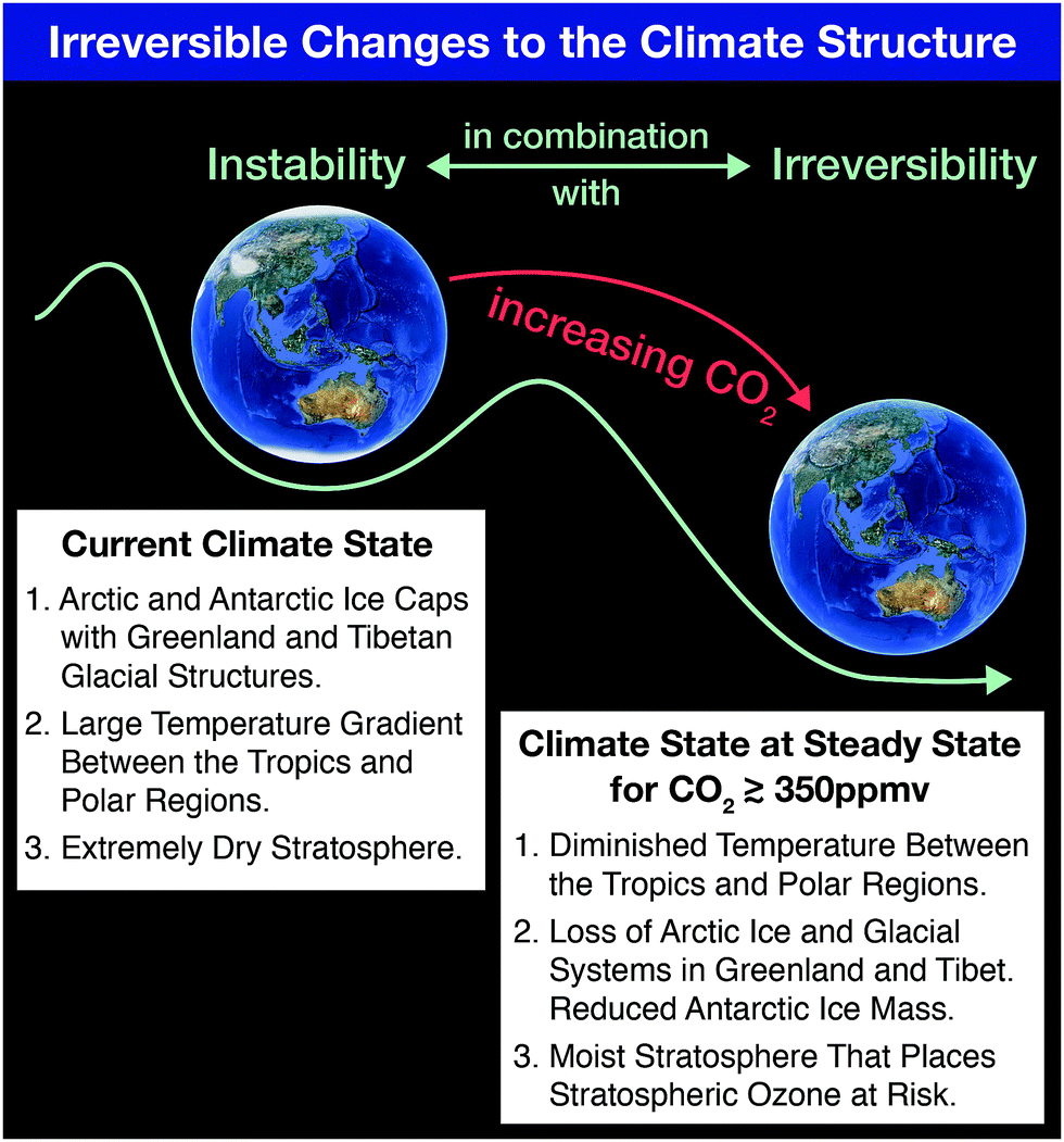 | ||
| Fig. 1 The current climate state characterized by polar ice systems in both hemispheres, a large temperature gradient between the tropics and the polar regions, in combination with a very dry stratosphere will, as the paleo-record demonstrates, transition to a markedly different climate state at CO2 mixing ratios greater than about 350 ppmv. That new climate state, in addition to more intense storm systems, is characterized by a sharply reduced temperature gradient between the tropics and polar regions, the absence of cryo-systems in the Northern Hemisphere, markedly higher sea levels and a moist stratosphere. | ||
1.2 Example of the importance of feedbacks in subsystems of the climate structure: the rapid loss of Arctic floating ice volume
The clearest manifestation of the importance of tracking heat flow into subsystems of the climate structure is reflected in the rapid changes to the Arctic system that emerge from observations of the remarkably rapid decrease in the volume of permanent floating ice in the Arctic Ocean in the last four decades. Fig. 2, panel A, summarizes the time evolution of the volume of Arctic floating ice based on the University of Washington Applied Physics Laboratory Polar Ice Observations Modeling and Assimilation (PIOMAS) results released periodically on the PIOMAS website. These important results track the Arctic Ocean ice volume through to the present beginning in 1979 when there was 17 × 103 cubic kilometers of floating ice at the end of the summer melt season (mid-September), referred to as the “permanent ice”. The ice volume by mid-September 2017 reveals that the ice volume has decreased to approximately 4 × 10³ cubic kilometers—a decrease of 75% in just 38 years. It is also important to underscore that both the first and second derivative of ice volume as a function of time are strongly negative. This is a direct result, and clear indicator of, the potent positive feedbacks within the Arctic cryo-structure itself.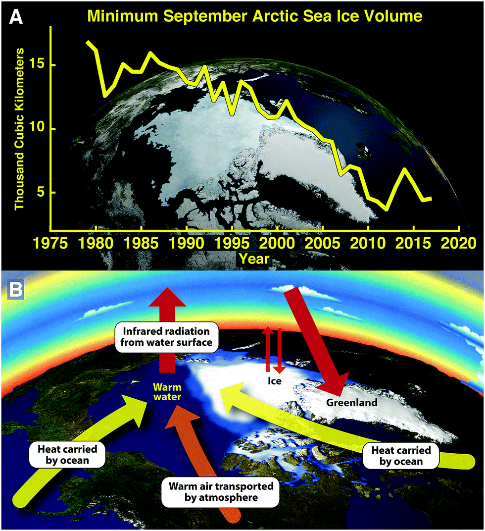 | ||
| Fig. 2 Perhaps the most dramatic impact on the global climate structure is the rapid loss of permanent floating ice volume in the Arctic Ocean displayed in panel A. Permanent ice refers to the ice volume that remains each year at the end of the summer melt season that has dropped from 17 × 103 km3 in 1979 to 4 × 10³ km3 in 2016. Panel B delineates the potent feedbacks that serve to set the time scale for the irreversible loss of Arctic floating ice that is reflected in the negative first and second derivatives of the ice volume displayed in panel A. Those feedbacks include the increased heat flow into the Arctic Basin delivered by the inflow of warm sea water from lower latitudes that increases as the ice cap constricts, the increased heat flow into the Arctic Basin delivered by the inflow of warm air as the ice and snow cover in the region surrounding the Arctic Basin is replaced by dark terrestrial vegetation and open ocean, and finally by the marked increase in the input of solar radiation to the surface water of the Arctic Ocean as the ice cap withdraws. | ||
As we will see in the next section this loss of Arctic permanent ice has major consequences for the overall global climate structure. This raises the immediate question: can the Arctic Ocean lose 75% of its permanent ice volume and recover to a stable climate state? The answer to this question is clearly no, because of the powerful feedbacks in the Arctic system that are represented graphically in Fig. 2, panel B. First of all, as the ice cap over the Arctic Ocean contracts, it allows warm low latitude ocean water to enter the Arctic Basin—in sharp contrast to the case in earlier decades when the Arctic Ice Cap covered the entire Arctic Basin, blocking the inflow of warm surface waters from lower latitudes. In addition, because the atmospheric transport of heat by wind systems entering the Arctic Basin was dramatically decreased by radiative cooling into the low temperature ice and snow fields covering regions surrounding the Arctic, little heat was transported via wind systems into the Arctic Basin. In sharp contrast, with the elimination of ice and snowcover from the region surrounding the Arctic Basin, a large flux of heat into the Arctic Basin results. These are the first two feedbacks that contribute to the increasing rate of disappearance with time of Arctic ice. Another important factor is the albedo effect—that ice and snow reflect 90% of the incoming summer solar shortwave radiation, whereas the exposed forests of the terrestrial component and the exposed water in the Arctic Ocean absorb 90% of the incoming shortwave solar radiation. This results primarily and most importantly in the warming of the surface waters of the Arctic Ocean in the summer that rapidly increases the rate of removal of ice. In the 1950s the average depth of the Arctic ice cap covering the Arctic Ocean was about 3.5 meters. Today, in sharp contrast, the average depth of the ice is a mere 1.5 meters which means that that remaining ice is sitting directly in the warm pool heated by the incoming solar radiation in the summertime.
Finally, the structure of the remaining ice is made up of small regions of ice connected via a web of very thin ice. The result is that the surface-to-volume ratio of the ice that remains is much greater than was the case with 3.5 meter thick monolith of ice and the result is that the remaining ice melts much more quickly in the early summer. In addition, the fragile nature of the remaining ice structure means that it is far more susceptible to wind conditions breaking up the remaining ice cover. Thus an impervious, largely immobile ice structure that characterized the Arctic since the last ice age has evolved into a far more delicate and unstable architecture that is rapidly crumbling.
1.3 Feedbacks within the global climate structure that couple directly to the Arctic
An important factor in the understanding of the global climate response to increased forcing of the climate by CO2 and CH4 is the cascade of feedbacks that emanate from the loss of ice volume from the Arctic Ocean. This underscores the fact that the Arctic as a system drives key feedbacks within the larger global climate structure. An example of this coupling is displayed in Fig. 3 that we will refer to repeatedly in linking climate change to chemical kinetics. First, as we have already noted, the feedbacks that accelerate the rate of permanent ice loss in the Arctic are comprised of heat transport by the ocean, heat transport by the atmosphere, and the increased absorption of solar radiation by the land and surface waters of the Arctic Basin. The warming surface waters of the Arctic Ocean emit radiation in the infrared (IR) proportional to the fourth power of the temperature and that bathes the entire Arctic Basin with increased infrared flux.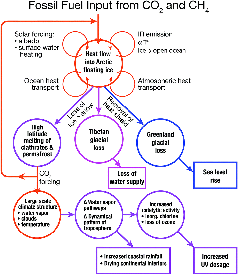 | ||
| Fig. 3 The cascade of coupled feedbacks that originate in the Arctic include the increasing rate of ice volume loss from the Greenland glacial system that serves to accelerate the rate of sea level rise, the increasing rate of ice volume loss from the Tibetan glacial system that threatens water supplies to China and India, the melting of methane clathrates and permafrost that increase the flux of greenhouse gas release from the Arctic Basin to the atmosphere, the warming surface waters of the world's oceans that intensify and increase the frequency of storm systems. One manifestation of increased storm intensity and frequency is the increasing depth and frequency of storm systems over the central United States in summer with the potential of triggering ozone loss in the stratosphere. | ||
Emanating from the feedbacks within the Arctic Basin itself is a manifold of coupled responses and feedbacks within the global climate structure. First, driven by the rapid warming of the Arctic Basin, is the melting of soil-based carbon reservoirs releasing both carbon dioxide and methane which serves to increasingly force the climate as a result of the trapping of infrared radiation. As we will see in subsequent sections, the decrease in the amount of Arctic ice removes a critical “heat shield” that has protected the Greenland glacial system for the last 120![[thin space (1/6-em)]](https://www.rsc.org/images/entities/char_2009.gif) 000 years since the last inter-glacial period by suppressing summer temperatures sufficiently to prevent any substantial mass loss of ice. Greenland, because it contains a volume of ice corresponding to 7 m of sea level rise, is a critically important consideration for forecast models of sea level rise. In contrast, the Tibetan glacial structure provides 65% of the summer flow of water to China and 90% of the summer flow of water to India. Just as the Arctic ice structure protects Greenland against melting, so too does the Arctic ice structure contribute to the protection of the Tibetan glacial system from mass loss.
000 years since the last inter-glacial period by suppressing summer temperatures sufficiently to prevent any substantial mass loss of ice. Greenland, because it contains a volume of ice corresponding to 7 m of sea level rise, is a critically important consideration for forecast models of sea level rise. In contrast, the Tibetan glacial structure provides 65% of the summer flow of water to China and 90% of the summer flow of water to India. Just as the Arctic ice structure protects Greenland against melting, so too does the Arctic ice structure contribute to the protection of the Tibetan glacial system from mass loss.
The next series of feedbacks we consider involve the large-scale dynamical changes to the climate structure that is set, in the current climate state, by the temperature difference between the tropical regions and the polar regions. As the loss of Arctic permanent ice occurs, the temperature of the polar regions of the northern hemisphere increase far more rapidly than does the average global surface temperature. This is typically termed the “Arctic Amplification”. This Arctic Amplification results in a fundamental shift in the atmosphere's overturning structure that engenders dynamical changes to the atmosphere that shifts climate regions pole-ward in each hemisphere. This implies, for example, the shift of the climate of Northern Africa into the Mediterranean Basin and the shift of the climate of Northern Mexico into the central United States.
A final feedback that will be discussed in the sections that follow involves the increasing surface temperatures of the ocean that leads to increased convective activity in severe storm systems, particularly the intensity of hurricanes and typhoons as well as the intensity or tornadoes and hail storms over the central United States. The increase in the intensity of the convective systems over the Great Plains of the United States in summer, provides the injection of water vapor deep into the stratosphere in July and August each year potentially resulting in the rapid heterogeneous catalytic conversion of inorganic chlorine (primarily HCl and ClONO2) to free radical form, ClO.3,4 This is particularly important in the chlorine system resulting in the increase in concentration of the ClO free radical that then engages the direct catalytic removal of ozone just as it does over the Antarctic and the Arctic in the winter. Except in this case it engenders O3 loss over the highly populated central United States in summer.
1.4 CO2 and CH4 release from melting permafrost and methane clathrate
Compounding the central role that the Arctic plays in setting the time scale for irreversibility regarding the global climate structure, are coupled feedbacks between the increasing temperatures resulting from increased heat flow into the Arctic Basin, and associated carbon release from melting permafrost and methane clathrates.5,6 The thinning and loss of the Arctic ice cap, as well as thawing permafrost, tap into the large carbon reservoirs containing both CH4 within clathrates and organic carbon within the terrestrial permafrost system. Methane clathrates are composed of cages of ice structures within which methane, released by the anaerobic decomposition of organic material, is trapped. A key measure of the importance of methane clathrates is reflected in the fact that these clathrates contain an amount of chemical energy two to three times the chemical energy contained in all deposits of petroleum, natural gas, and coal combined worldwide.7As the Arctic Basin melts in response to increasing temperatures, carbon in surface soils will be released as CH4 and CO2 as the depth and geographic range of melt zones increase. For a point of reference, the release of 0.5% of the labile carbon in the upper 3 meters of the Alaska North Slope and Northern Siberia per annum equals the total carbon released to the atmosphere from all fossil fuel extraction, distribution and combustion per annum.
Fig. 4 displays, in the insert, the structure of methane clathrate as well as its combustion. Fig. 4 displays the Intergovernmental Panel on Climate Change (IPCC) analysis tracking the release of carbon added to the atmosphere each year from fossil fuel use for different release scenarios. The actual carbon addition to the atmosphere from fossil fuel use is displayed in the figure since 2007—an amount that exceeds in each year the IPCC projected maximum release rate.8,9
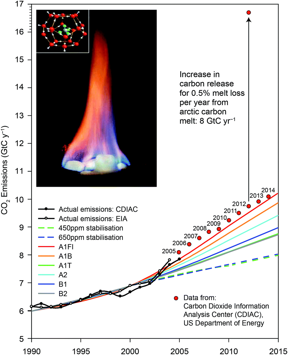 | ||
| Fig. 4 An important consideration is to compare the fraction of the labile carbon contained in the upper 3 meters of the soils in Northern Siberia and the North Slope of Alaska with that of the total carbon dioxide released worldwide by the extraction, distribution and combustion of fossil fuels. As noted in the figure, just 0.5% of that labile carbon equals the total mass of carbon added to the atmosphere as CO2 from fossil fuel use. | ||
A brief examination of the carbon reservoirs in the Arctic reveals the urgency in quantifying carbon fluxes from this region. While the entire human enterprise now contributes ten gigatons of carbon to the atmosphere each year (GtC per year), the Arctic soil reservoir represents between 1400 and 1850 GtC in the upper 3 meters of the soils of the Alaskan North Slope and in Northern Siberia.10,11 The reservoirs of methane trapped as gas hydrates are between 30 and 170 Gt-CH4 and between 5 and 195 Gt-CH4 for the Arctic Ocean in Arctic permafrost regions, respectively. If just 0.5% of the Arctic carbon reservoir is liberated as CO2 and CH4 each year, it will add another 8 Gt to the atmosphere, dramatically adding to the radiative forcing of the climate. The potential for a rapid and irreversible increase in carbon emissions from the Arctic places major importance on establishing both the high spatial resolution flux of CO2 and CH4 as well as the mechanism for this release in order to develop tested and trusted forecasts of carbon release in the years and decades ahead. Understanding of carbon release from the Arctic Basin is an imperative.
1.5 Increased heat flow into the Greenland glacial structure that accelerates sea level rise
While the Greenland glacial structure has survived intact since the last interglacial period 120000 years ago, the loss of permanent ice in the Arctic has initiated a dramatic change in conditions on Greenland as the time series of satellite observations of surface water12 and an analysis of ice mass loss from Greenland13 have made clear. Fig. 5, panel A, tracks the formation of summer surface water from 1992 through 2012. Panel B of Fig. 5 highlights the fact that the surface melt water on Greenland flows downward through fissures in the ice structure, breaking the bond between the glacial system and the bedrock. This destabilizes the ice structure and accelerates the decomposition of the glacial system by weakening the horizontal confinement of the ice structure such that it collapses outward and downward. This in turn increases the rate of sea level rise because the reduction in glacial volume results not from the slow melting of a monolithic ice structure, but rather from the collapse of the entire glacial system that can occur far more rapidly than simple melting. Panel C of Fig. 5 represents just one example: the impact on the state of Florida for a 3 meter rise in sea level corresponding to 40% of the ice volume of Greenland. As the sophistication of the forecast models increases—incorporating improved physics into the glacial dynamics of ice flow and breakup—the amount of sea level rise forecast by the end of the century has increased to between 1.5 and 3 meters, with a probability tail extending to 6 to 7 meters of sea level rise.14,15 These forecasts include contributions from the melting of the Antarctic glacial structures that contain an ice volume equal to 70 meters of sea level rise.
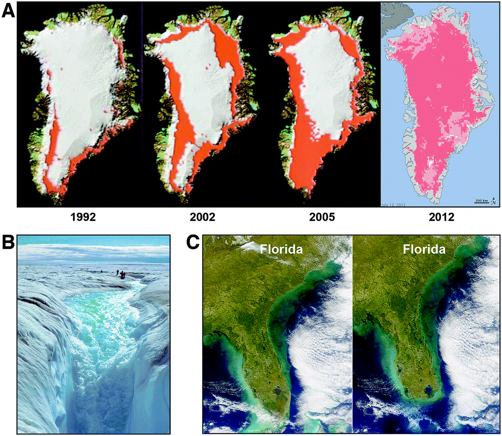 | ||
| Fig. 5 Satellite observations of the melt water on the surface of the Greenland glacial system is shown in red in panel A tracing the increase in surface water from 1992 to 2012. Prior to the late 1980s, there was no significant surface water on the Greenland glacial system. Panel B shows the down-flow of water from the glacial surface of Greenland that occurs through “moulins” that duct the melt water directly to the bedrock that serves to break the bond between the ice and the bedrock, accelerating the collapse of the ice structure. While Greenland alone contains an ice volume equal to 7 meters of sea level rise, just a 3 meter rise submerges the southern quarter of the state of Florida as displayed in panel C. | ||
1.6 Coupling increasing levels of CO2 and CH4 to the free radical kinetics controlling ozone loss over the central United States in summer
As the surface waters of the Gulf of Mexico increase in temperature as a direct response to increasing concentrations of CO2 and CH4 in the atmosphere, exponentially more moisture enters the low-level jet that carries the moisture northward over the central United States where convection is initiated as the river of air ascends over the Great Plains, triggering explosive convection. The resulting severe storms produce convection reaching 6 to 8 kilometers into the stratosphere where the mixture of water and radical precursors from the boundary layer enter the anticyclonic gyre that results from the North American monsoon. This initiation of the flow of warm moist air from the warming surface waters of the Gulf of Mexico is displayed in Fig. 6 along with the anti-cyclonic gyre also displayed in Fig. 6 that serves to capture the convectively injected mixture of water vapor and radical precursors for periods of up to two weeks in July and August, creating a “batch reactor” that allows time for the catalytic removal of ozone to occur. The analysis of the kinetics of free radical catalyzed loss of stratospheric ozone is treated in the following sections.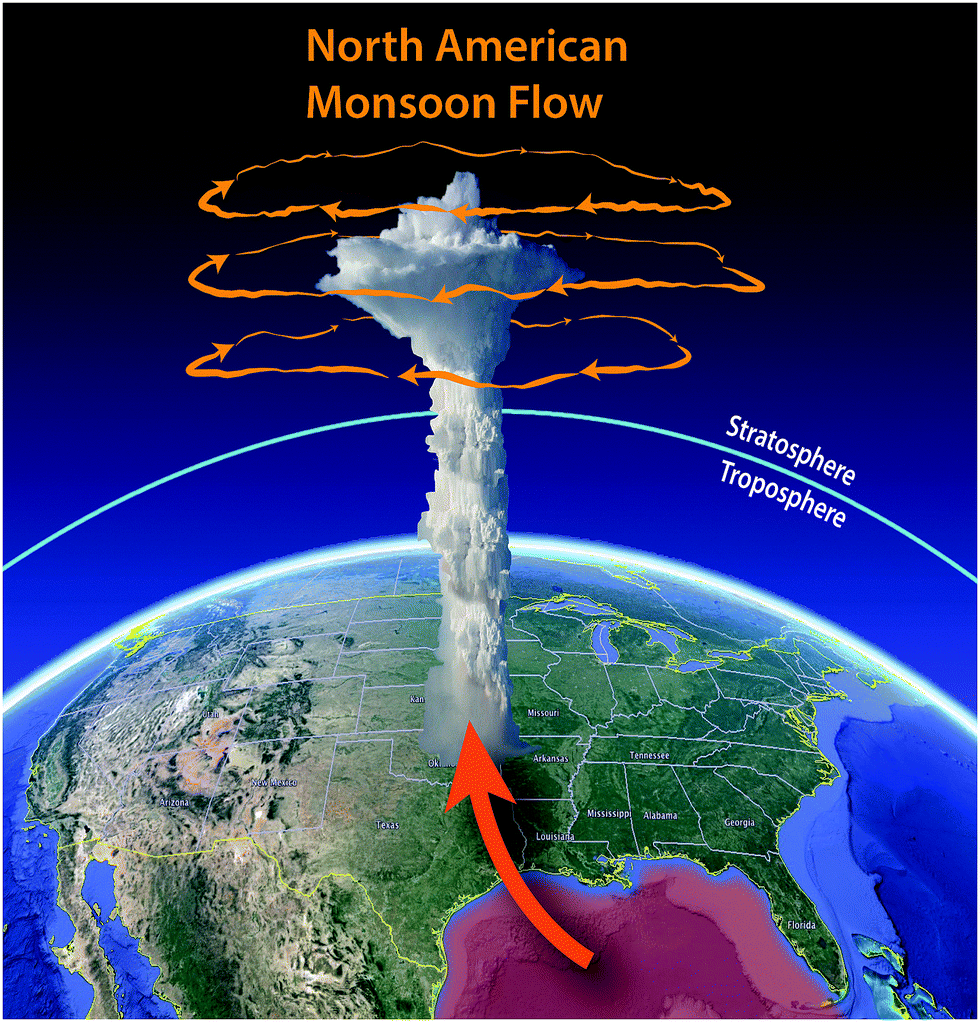 | ||
| Fig. 6 The warming surface waters of the Gulf of Mexico feed increasing moisture to the low-level jet that delivers water to the central United States in summer, intensifying the convective power of storms that inject water vapor deep into the stratosphere, entering the anti-cyclonic gyre that sequesters the injected mixture of water and radical precursors allowing time for the catalytic loss of ozone. | ||
2. Coupling of radical catalyzed loss of stratospheric ozone to climate forcing by increased CO2 and CH4 in the atmosphere
2.1 Overview: new observations and mechanistic analysis of catalytic processes
An array of recent observational evidence4 has brought renewed focus on the dynamical and photochemical mechanisms that control ozone in the lower stratosphere over the United States in summer. In particular, the coupling of six factors, when considered in specific combinations, define why the central US in summer represents a unique case, in the global context, of the risk of regional ozone loss. These factors, depicted in Fig. 7, include: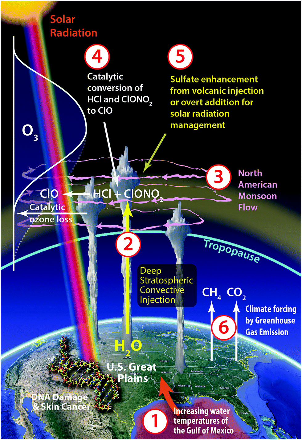 | ||
| Fig. 7 In the context of climate-chemistry coupling globally, the central US in summer represents a combination of factors specific to both the geographic region and the season. Northerly flow of warm moist air from the Gulf of Mexico in combination with heating and convergence over the Great Plains frequently triggers powerful convection that injects water vapor into the stratosphere, where the upper level anti-cyclonic flow associated with the NA monsoon can sequester the injection for a week or more over the US. This, in combination with cold stratospheric temperatures, can lead to heterogeneous catalysis on ubiquitous sulfate–water aerosols that converts inorganic chlorine to ClO and can initiate ozone loss through an array of gas-phase catalytic cycles. Potential future enhancements in sulfate from volcanic injection or geoengineering increase the likelihood of halogen activation and ozone loss. | ||
(1) Warming surface waters of the Gulf of Mexico that induce increased water vapor carried by the low-level jet that feeds warm, moist air to the lower atmosphere over the central United States inducing in turn;
(2) development of severe storm systems over the Great Plains of the US with convective cores that extend well above the tropopause, leading to the injection of water vapor and possibly halogen radical precursors deep into the stratosphere;16–19
(3) anti-cyclonic flow in the stratosphere over the US in summer, associated with the North American monsoon (NAM), that serves to increase the retention time of the convectively injected species over the US20,21 creating in effect a photochemical batch reactor;
(4) increased probability for the catalytic conversion of inorganic chlorine (primarily HCl and ClONO2—hereafter Cly) to free radical form (ClO) on ubiquitous sulfate aerosols due to a combination of gravity wave induced ambient temperature perturbations and localized water vapor enhancements, which can accelerate the catalytic removal of ozone in the lower stratosphere;17,22
(5) potential for future sulfate enhancements from volcanic eruptions23–26 or overt addition by the geoengineering approach of reducing solar forcing by increasing albedo via solar radiation management (SRM);27–32
(6) and increased forcing of the climate by continued CO2 and CH4 emissions from the extraction, transport and combustion of fossil fuels, that has the potential to increase the frequency and intensity of storm systems over the Great Plains in summer.33–36
In this section we present observations that define:
(a) the frequency and depth of convective penetration into the stratosphere of condensed phase water over the central US in summer employing the NEXRAD weather radar system,
(b) available inorganic chlorine placed within the same vertical coordinate system as the NEXRAD observations,
(c) high accuracy, high spatial resolution in situ observations of the temperature structure of the lower stratosphere over the US in summer that clarify the importance of spatial and structural variability and gravity wave propagation on the heterogeneous catalytic conversion of inorganic chlorine to free radical form, and
(d) to use the observations of convective penetration heights, elevated water vapor, and temperatures as inputs to a photochemical model,24,37–39 which calculates concentrations of the rate limiting ClO, BrO, HO2 and NO2 radicals that control the catalytic loss rate of ozone and the resulting fractional decrease in ozone.
The context for the analysis presented here concerns the issue of human health associated with the remarkable sensitivity of humans to small increases in UV dosage that initiate skin cancer. In particular, diagnosed cases of basal cell and squamous cell carcinoma have reached 3.5 million annually in the US alone.40–43 The analysis presented here of the sensitivity of lower stratospheric ozone over the US in summer builds on four decades of developments linking chlorine and bromine radicals to ozone loss in the polar regions,44,45,55 and to ozone depletion at mid-latitudes resulting from the coupling of volcanic aerosols and temperature variability to anthropogenic chlorine and bromine,22,24,25,56 as well as analyses of the consequences from sulfate addition to the stratosphere from geoengineering via solar radiation management.29–32 Finally, while detailed simultaneous observations of the key catalytic free radicals, reactive intermediates and ozone loss rates have been thoroughly investigated in the stratosphere over the Antarctic and Arctic in winter, the same is not the case for the stratosphere over the US in summer.
2.2 Photochemical framework for catalytic ozone loss in the lower stratosphere
Studies of catalytic ozone loss in the lower stratosphere at high latitudes established the network of catalytic reactions linking inorganic chlorine to the rate of ozone loss in the lower stratosphere. Simultaneous in situ aircraft observations of ClO, BrO, ClOOCl, ClONO2, HCl, OH, HO2, NO2, particle surface area, H2O and O3 in the transition through the boundary of the Arctic vortex49–52 showed explicitly the loss of ozone as well as the distinct anti-correlation between the concentration of the rate limiting radical ClO and the ozone concentration. It is the chlorine monoxide radical, ClO, in combination with the rate limiting step (RLS) ClO + ClO + M → ClOOCl + M in the catalytic cycle first introduced by Molina and Molina46 and the catalytic cycle rate limited by ClO + BrO → Cl + Br + O2 first introduced by McElroy et al.47 that constitute the reaction mechanisms capable of removing ozone over the polar regions in winter at the observed rates.48,53,54A distinguishing feature of the regime within the polar jet, which defines the boundary of the Arctic vortex in winter, is that temperatures within the vortex are lower by approximately 6–7 K than outside the vortex. This modest suppression in temperature is adequate to trigger the heterogeneous catalytic conversion of Cly to Cl2 and HOCl at H2O mixing ratios of 4.5 ppmv on simple, ubiquitous sulfate aerosols.22,57–60 The Cl2 and HOCl products of Cly heterogeneous catalysis on sulfate aerosols45 photodissociate to produce Cl atoms that react with O3 to produce ClO. Hereafter, we refer to this series of reactions as the conversion of Cly to ClO.
Examination of conditions in the Arctic lower stratosphere coupled with extensive results from laboratory experiments and modeling57–60 have set in place the temperature-water vapor-sulfate coordinate system defining the regime of rapid heterogeneous conversion of Cly to ClO.57Fig. 8 displays a schematic illustrating the temperature-water vapor threshold between the domain in which conversion of inorganic chlorine to its catalytically active forms becomes significant (shaded region) and the temperature-water vapor domain that leaves inorganic chlorine bound in its reservoir species (unshaded region).57–60 Probabilities (γ's) associated with the heterogeneous reactions considered here are sensitive to aerosol composition.57–60 In particular, reactions involving HCl are governed by its uptake and solubility, which are strongly dependent on both the sulfuric acid weight percent of the aerosol and temperature. As the sulfuric acid weight percent decreases, the solubility of HCl increases. The sulfuric acid weight percent is itself a function of relative humidity. With shifts to colder temperatures and/or higher water vapor mixing ratios leading to more dilute sulfate within the aerosol, the reaction probabilities for the conversion of Cly to ClO increase exponentially. Therefore, wherever the specific conditions of temperature and water vapor are satisfied, the heterogeneous catalytic conversion of Cly to ClO can occur on the simple, ubiquitous binary aerosol, and ozone loss can result.
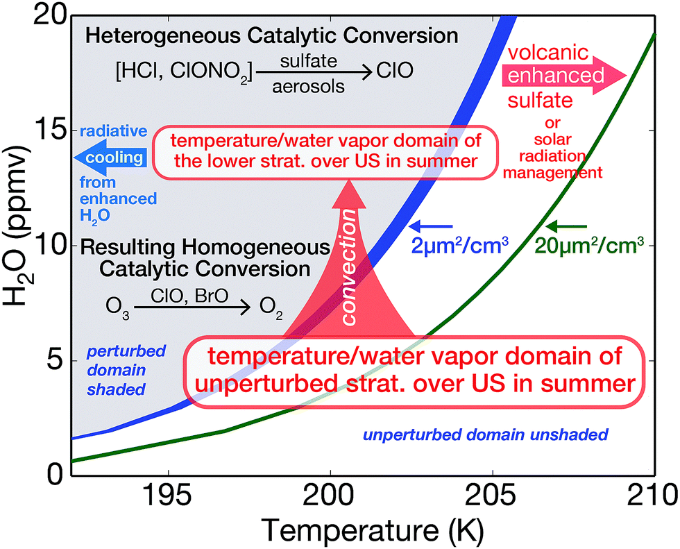 | ||
| Fig. 8 An example of the three-dimensional dependence of heterogeneous catalytic conversion of inorganic chlorine (Cly ≈ HCl + ClONO2) on temperature, water vapor and sulfate loading is displayed in a manner that distinguishes rapid conversion of Cly to free radical form in the shaded region (with the threshold defined as 10% chlorine activation in the first diurnal period) from the unshaded region for which there is virtually no Cly to ClO conversion. This establishes the photochemical framework for the analysis of convective addition of water, sulfate addition by volcanic injection or overt sulfate addition for solar radiation management (SRM), or combinations thereof. The broad blue line dividing the perturbed and unperturbed domains corresponds to a sulfate reactive surface area of 2 μm2 cm−3; the green line represents a shift in sulfate reactive surface area to 20 μm2 cm−3. | ||
The cornerstone of our understanding of sulfate–halogen induced reductions in ozone over mid-latitudes of the northern hemisphere (NH) is built upon observed column ozone loss following the 1991 eruption of Mt. Pinatubo.22,24–26 The impact of the volcanic eruption on ozone extended over a period of nearly four years following the eruption when column ozone concentrations over the NH decreased by a maximum of 5% in the latitude region 35–60°N.24 Model analysis of the impact emphasized the central role of halogen radical catalytic loss of ozone, particularly the important role of bromine radicals in the lower stratosphere at elevated levels of sulfate aerosol loading.24 The addition of sulfate to the stratosphere by either volcanic injection or overt addition for SRM is indicated in Fig. 8 as the sulfate “shift” to the green line that serves to expand the domain for rapid heterogeneous catalytic conversion of Cly to ClO. Radiative cooling to space from the domain of enhanced water vapor is displayed with the blue arrow in Fig. 8.
The four catalytic cycles that must be taken into account in the assessment of ozone loss rates in the lower stratosphere include the most important rate limiting steps under unperturbed as well as perturbed conditions, i.e., conditions of elevated water vapor or lower temperatures. In this analysis “unperturbed” refers to background sulfate loading of 1–3 μm2 cm−3 and a water vapor mixing ratio of 4.5 ppmv. The four dominant rate limiting catalytic steps include: (1) ClO + ClO + M → ClOOCl + M, (2) BrO + ClO → Br + Cl + O2, (3) NO2 + O → NO + O2 and (4) HO2 + O3 → OH + 2O2. Under unperturbed conditions in the lower stratosphere between 10 and 22 km, the catalytic loss of ozone is dominated by the HO2 + O3 → OH + 2O2 RLS, as originally demonstrated by Wennberg et al.61 The ClO + BrO cycle plays a significant role (∼15%), exceeding the ClO dimer catalytic cycle by more than an order of magnitude under unperturbed conditions. Above approximately 22 km, the catalytic cycle rate limited by NO2 + O → NO + O2 becomes dominant. The rate limiting catalytic species ClO, BrO, HO2 and NO2 thus constitute the baseline against which unperturbed conditions may be contrasted relative to perturbed cases involving temperature variability and the convective injection of water vapor.
2.3 NEXRAD weather radar map of storm-top height geographic distribution and penetration depth into the stratosphere over the US in summer
The Next-Generation Radar (NEXRAD) weather radar network has markedly advanced our understanding of both the frequency and depth of tropopause-penetrating convection in the lower stratosphere over the US in summer. Prior to the radar analysis methods applied by Solomon et al.62 for mapping the 3D structure of convective penetration, elevated water vapor mixing ratios in the stratosphere were observed in situ during multiple summertime aircraft missions over the US.16,17,63 These observations of both vapor phase H2O and the HDO isotopologue, obtained aboard NASA's WB-57 and ER-2 aircraft, provide direct evidence of water vapor deposited by convection in the stratosphere. Maximum water vapor values observed in situ range from 8 to 18 ppmv for individual plumes typically sampled a day to a few days after convective injection. In support of the in situ observations, the NEXRAD weather radar data provide compelling statistics on the frequency, 3D structure, and high accuracy determination of the storm-top altitude of convection.Solomon et al.62 used radar analysis methods and observations from the operational NEXRAD radar network to create a high-resolution, three-dimensional, gridded radar reflectivity product for 2004 over the conterminous US east of the Rocky Mountains. By combining the NEXRAD analysis with the lapse-rate tropopause height derived from the European Center for Medium-Range Weather Forecasting ERA-Interim reanalysis, they produced high-resolution maps of convection overshooting the tropopause level at 3 hour intervals for the entire year. The ERA-Interim estimates of the tropopause altitude agree well with high vertical resolution observations from radiosondes.64 These ice-rich overshooting parcels lead to injection of water vapor into the stratosphere through mechanisms including turbulent mixing and gravity wave breaking.64
The geographic distribution of overshooting events is markedly non-uniform, with the great majority occurring east of the Rocky Mountains and west of the Mississippi River. The largest concentration of overshooting events occurs over the high plains stretching from Texas to Nebraska and Iowa. The ongoing analysis of a 10-year hourly NEXRAD dataset for May through August of 2004 to 2013 confirms the diurnal, annual, and geographical patterns found by Solomon et al.62 A key contribution that the NEXRAD system provides is the ability to map the storm-top potential temperature as a function of geographic position, frequency and month of occurrence. The multi-year analysis indicates that 38158 storms reached at least 2 km above the tropopause over the central US in May–August between 2004 and 2013, with about 50% of these extending above the 390 K potential temperature level (approximately 16 km). The depth and frequency of penetration has significant consequences, so we delineate here the quantitative specifics of the NEXRAD observations with high spatial resolution values of HCl that inform the altitude-dependent distribution of available inorganic chlorine.
The vertical coordinate system most appropriate for the quantitative coupling of the NEXRAD observations to that of inorganic chlorine is potential temperature (the temperature of an air parcel compressed adiabatically to 1000 hPa) because, in the absence of diabatic processes, air parcels in the stratosphere are transported along surfaces of constant potential temperature, such that long-lived trace species exhibit consistent correlations with one another. In particular, this is a characteristic shared by long-lived tracers that are either produced or removed by increasing UV radiation as a function of increasing altitude in the stratosphere, e.g., HCl vs. O3 and Clyvs. N2O. Data from multiple in situ measurement campaigns, as well as satellite retrievals, have been used to quantify the relationships among these species.54,65 In Fig. 9, high resolution vertical profiles of HCl mixing ratio (blue data points) were inferred from in situ measurements of O3 using the linear relationship between Aura Microwave Limb Sounder (MLS) measurements of HCl and O3 at 100 hPa and 68 hPa, such that HCl (pptv) ≈ 7.0 × 10⁻⁴ × O3 (pptv). MLS version 4.2 data from 2004–2016, sub-selected to be between 30°–50°N and 80°–105°W for June through August, were used to derive this conversion factor. The in situ O3 data used to calculate HCl throughout the lower stratosphere over the US in summer are from the NASA Studies of Emissions and Atmospheric Composition, Clouds, and Climate Coupling by Regional Surveys (SEAC4RS) mission, which took place over the US in the summer of 2013. Shown in Fig. 9 are in situ measurements of HCl from the NASA AVE campaign over the US in June 2005 as the array of black data points. HCl comprises most of the inorganic chlorine in the lower stratosphere, and accordingly, Fig. 9 demonstrates the rapid rise in available inorganic chlorine with increasing potential temperature (altitude).
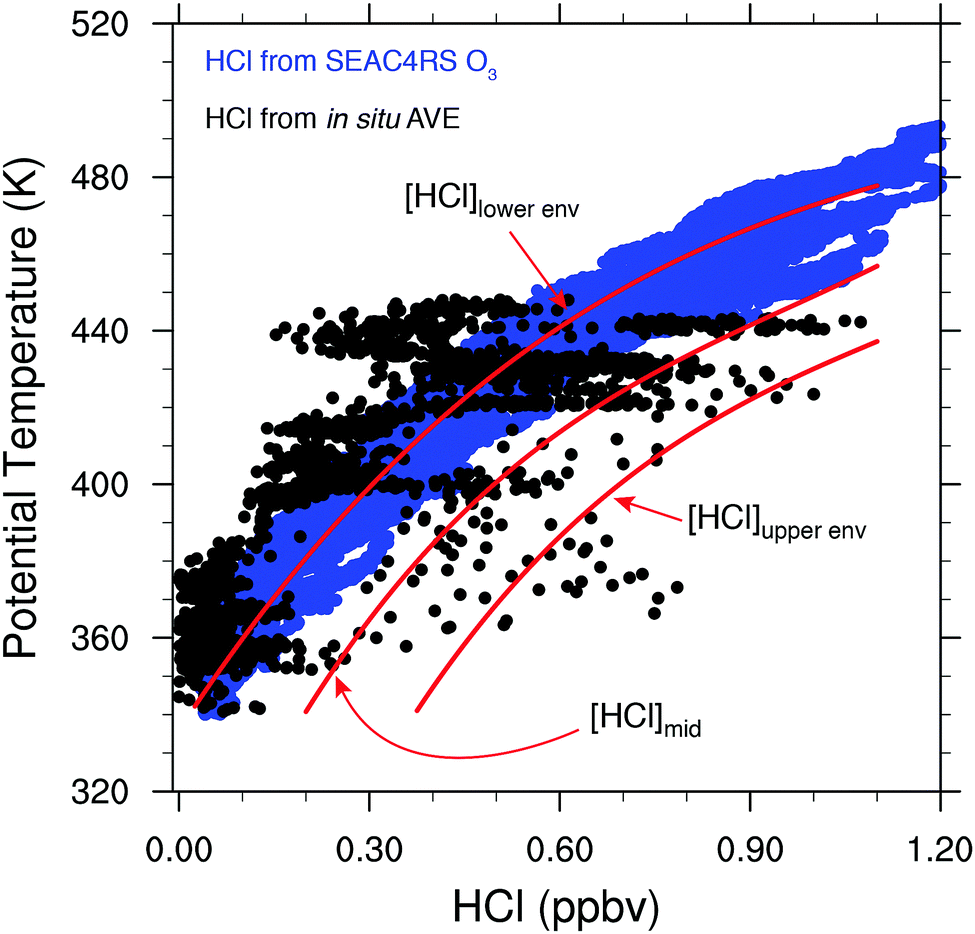 | ||
| Fig. 9 The profile of HCl mixing ratio with height is displayed where the nested blue points trace out HCl calculated using in situ O3 data from the NASA SEAC4RS mission (see text). The black points are in situ observations obtained with the Chemical Ionization Mass Spectrometer (CMIS) instrument during the NASA Aura Validation Experiment (AVE) mission in June of 2005. Data acquired between 30° and 50°N latitude and 80° and 110°W are displayed. The curved red lines represent the three ranges of HCl: [HCl]lowerenv, [HCl]mid, and [HCl]upperenv used in the calculations of ozone loss. | ||
In order to appraise the quantitative impact on ozone catalytic loss rates of variations in both temperature and convectively injected water vapor, three profiles of the HCl mixing ratio are chosen to represent the range in observed HCl: [HCl]lowerenv and [HCl]upperenv that represents the lower and upper bound of HCl in situ observations, and [HCl]mid that represents the midpoint of HCl in situ observations.
Subsequent to the high in situ water vapor observations reported by Anderson et al.,3,4 Schwartz et al.66 analyzed satellite observations of water vapor from MLS and confirmed that the lower stratosphere over the United States in summer is indeed unusually wet, with measured values reaching as high as 18 ppmv. The MLS satellite data indicate that the highest stratospheric water vapor mixing ratios at the highest latitudes globally are over the central and eastern US in summer. These results are particularly noteworthy, because the true magnitude and number of water vapor enhancements over the US in summer is likely significantly greater than reported by the MLS satellite instrument. The reason is that elevated H2O from convective injection is localized in space and typically layered vertically, such that the spatial resolution of MLS (e.g., 3 km vertical × 200 km horizontal at 100 mb for H2O) may often exceed the dimensions of the perturbation or randomly transect it, leading to an underestimate of the mixing ratio. For example, a 2 km deep layer of elevated water of 50 km horizontal extent, even with optimal alignment of the convected geometry along the north–south viewing track of MLS, will only fill 1/6 of the MLS sample volume with the other 5/6 filled with background levels of H2O. This results in a substantial underreporting of the actual H2O mixing ratio present within the convected domain. Nevertheless, Schwartz et al.66 established the crucial fact that the stratosphere over the central and eastern US is unique globally with respect to significantly elevated water vapor.
Another key piece of evidence relating the observations of enhanced water vapor to their convective source comes from the ACE-FTS satellite observations of the concentration of the heavy water isotopologue HDO globally in the lower stratosphere67 as well as in situ observations of HDO within regions of convective injection from NASA aircraft missions. The HDO to H2O ratio is expressed in the usual isotopic formulation of δD that is reported in per-mil units and defined as δD (‰) = (Robs/RSMOW − 1) × 1000 where R = [HDO]/[H2O], “SMOW” refers to standard mean ocean water, and RSMOW = 3.12 × 10⁻⁴. Observations of δD are important because convective injection followed by sublimation is characterized by less negative values of δD in water vapor compared to air that has passed through the tropical tropopause, which has δD values of around −650‰. This corresponds to a 65% depletion of HDO relative to standard mean ocean water. In situ aircraft measurements of convective outflow show δD values of −200‰.68 The ACE-FTS global observations of δD at 16.5 km from Randel et al.67 show δD values of ∼−490‰ over North America but virtually no enhancement of δD over the global mean at 16.5 km altitude in any other geographic domain, including the Asian monsoon region. This is direct evidence for the convective source of water vapor in the stratosphere over the US in summer as well as for the unique occurrence of deep stratosphere-penetrating convection in the global context.
2.4 Observations of temperatures in the lower stratosphere over the US in summer
We employ high spatial resolution, high accuracy in situ temperature measurements acquired in the specific altitude, latitude, longitude and season appropriate for calculations of localized ozone loss in the lower stratosphere over the central US in summer.4 These temperature data were acquired aboard the NASA ER-2 high altitude aircraft on flights in the stratosphere during August and September 2013 over the central US during the NASA SEAC4RS mission. For the present analysis, which focuses specifically on the central US east of the Rocky Mountains, we select temperature data in the latitude range from 30° to 50°N and in longitude from 110° to 80°W. Three temperature curves, shown in Fig. 10, were selected to illustrate the extreme sensitivity to colder temperatures of the catalytic mechanisms that determine the rate of ozone loss under perturbed conditions. The three temperatures that we consider are: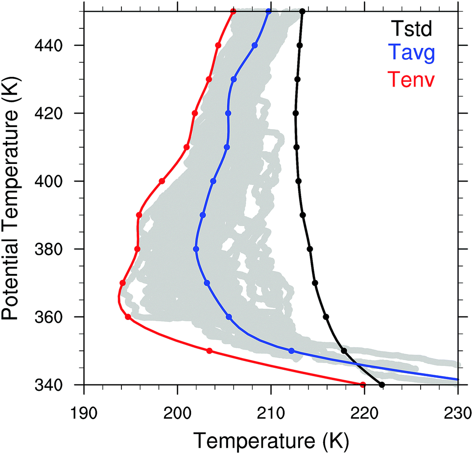 | ||
| Fig. 10 Three temperature profiles are used in the calculations of ozone catalytic loss. The temperature distribution Tstd displayed in black is a standard temperature typically used in 2D and 3D models, Tavg is the average of the observed temperatures obtained by high accuracy in situ aircraft measurements over the central United States in summer, and Tenv is the envelope of aircraft observed in situ temperature observations that reflect the amplitude of the temperature oscillation resulting from the propagation of gravity waves through the stratosphere. The period of oscillation of the temperature for a single gravity wave is on average 6 to 7 hours. The period of time for the heterogeneous catalytic conversion of HCl to ClO is on the order of a few hours, so the constant series of gravity waves traversing the stratosphere place particular importance on the envelope temperature Tenv in the analysis of the kinetics of ozone catalytic loss in the stratosphere over the US in summer. | ||
• Tstd that represents a standard temperature typically employed in stratospheric modeling,
• Tavg that is the actual observed average temperature obtained from the in situ aircraft observations over the central United States in summer, calculated by averaging the data over 10 K potential temperature bins centered on the isentropic level of interest, and
• Tenv that is the envelope of temperatures observed in situ by the aircraft that traces the observed temperature excursions resulting from the propagation of gravity waves through the stratosphere.
Because the catalytic conversion of HCl and ClONO2 (i.e. Cly) to ClO occurs in a matter of a few hours under perturbed conditions of convectively injected water vapor, combined with the fact that the average period of the gravity wave oscillation is in the range 6 to 7 hours, the Tenv temperature is the most important for the analysis of the heterogeneous catalytic chemistry converting Cly to ClO. The central objective in the analysis of the temperature dependence of the catalytic chemistry is to demonstrate the extreme sensitivity to temperature within the range of the observed temperatures. The observed temperatures from the aircraft in situ measurements are displayed as the gray dots in Fig. 10.
In the following modeling analysis, the three different temperature profiles, Tstd, Tavg, and Tenv, are employed to evaluate the response of the rate limiting steps for the catalytic loss of stratospheric ozone to (a) temperature alone in the absence of enhanced convectively increased water vapor, (b) the amount of convectively injected water vapor expressed in terms of the mixing ratio of water vapor, and (c) the amount of HCl present in the atmosphere prior to convective injection of water vapor. The amount of HCl present in the stratosphere over the central United States is seasonally dependent as HCl is enhanced by the equatorward flow from high latitudes following the breakup of the Arctic vortex. The diabatic cooling within the Arctic vortex during winter brings the HCl rich air to lower altitudes.
Fig. 10 defines the range in observed temperatures in the lower stratosphere over the central US in summer. Spatial and structural variability in combination with gravity waves that continuously traverse the lower stratosphere over the Great Plains in summer contribute to the observed temperature variability. These gravity waves are induced by strong convective events embedded in mesoscale convective systems (MCSs), squall lines and tornadic storm structures, as well as the presence of the Rocky Mountains.69 Also potentially contributing to the temperatures in the domain of elevated water vapor from convective injection is the radiative cooling of the region of enhanced water vapor to space at a rate of ∼0.5 K per day per 10 ppmv of additional water vapor.70,71 Given the remarkable non-linearity of the heterogeneous catalytic processes that control HCl to ClO conversion, the temperature observations are critically important for the determination the rate of catalytic loss of ozone.
2.5 Dynamics defining lower stratospheric flow patterns over the US in summer
The North American monsoon creates a situation during July and August that is particularly conducive to the hydration of the lower stratosphere by extremely deep convection. Not only does it steer water vapor from the Gulf of Mexico across Texas and into the western Plains States in the lower atmosphere, it also generates an anticyclone in the upper troposphere and lower stratosphere that causes stratospheric air parcels to dwell markedly longer over North America than if they were advected by a purely zonal flow. This anticyclonic circulation is not stable, though, leading to regular ventilation. Thus the mean residence time of air over the US ranges from one to two weeks with some parcels residing significantly longer.72 This sets the range of timescales for evaluating ozone loss over this region from one or more of these injections. Evidence that parcels are induced to circulate in a stratospheric anticyclone over North America during summer with convectively injected water vapor retention within the gyre is evident in tracer–tracer21 and satellite data.73–75 It is important to note that while the heterogeneous catalytic conversion of Cly to ClO on sulfate–water aerosols takes but a few hours following convective injection, the subsequent homogeneous catalytic loss of ozone takes place in the subsequent days and weeks following convective injection.2.6 Model calculations exploring the sensitivity of the rate limiting steps in the dominant ozone loss processes to perturbations in temperature and water vapor
Given the remarkable temperature sensitivity and non-linearity of the heterogeneous catalytic conversion of Cly to ClO on sulfate aerosols, and the sensitivity of ozone loss rates to changes in the concentrations of the rate limiting radicals ClO, BrO, HO2, and NO2, we model the stratospheric ozone system over the central US with a one dimensional chemical kinetics model used to simulate the conditions at various isentropic (constant potential temperature) levels for a stratospheric background condition derived from a regional and seasonal average. The range of potential temperatures considered extends from 340 K to 430 K (approximately 12 to 18 km). Background stratospheric concentration potential temperature profiles of relevant chemical species were obtained from a decadal and regional average of Aura-MLS satellite data in the summer months (June, July and August) of 2004 to 2013 in the central US defined as 30°N to 50°N and 110° to 80°W for HNO3, H2O, and O3. Background profiles for NO2, NO and inorganic bromine were obtained from in situ observations. Each background chemical profile was interpolated to the model potential temperature surfaces. The chemical model tracks 32 chemical species and 67 reactions. Most important of these reactions are the free radical cycles that destroy stratospheric ozone: the HOx, NOx and ClOx cycles. Of particular importance are the initiation reactions of the ClOx cycle and the heterogeneous activation of inorganic chlorine, due to their sensitivity to both water vapor concentration and temperature. The model state is defined by the chemical species concentrations and is integrated forward in time using the LSODA ordinary differential equation (ODE) solver. The LSODA program was selected for its ability to utilize both stiff (backward differentiation formula) and non-stiff (Adams) methods. An adaptive time step was also implemented over the integration period. Each potential temperature level was simulated independently for a time period of two weeks using three different temperature profiles and water vapor concentrations of 5 ppmv (stratospheric background), 10 ppmv and 20 ppmv (convectively influenced).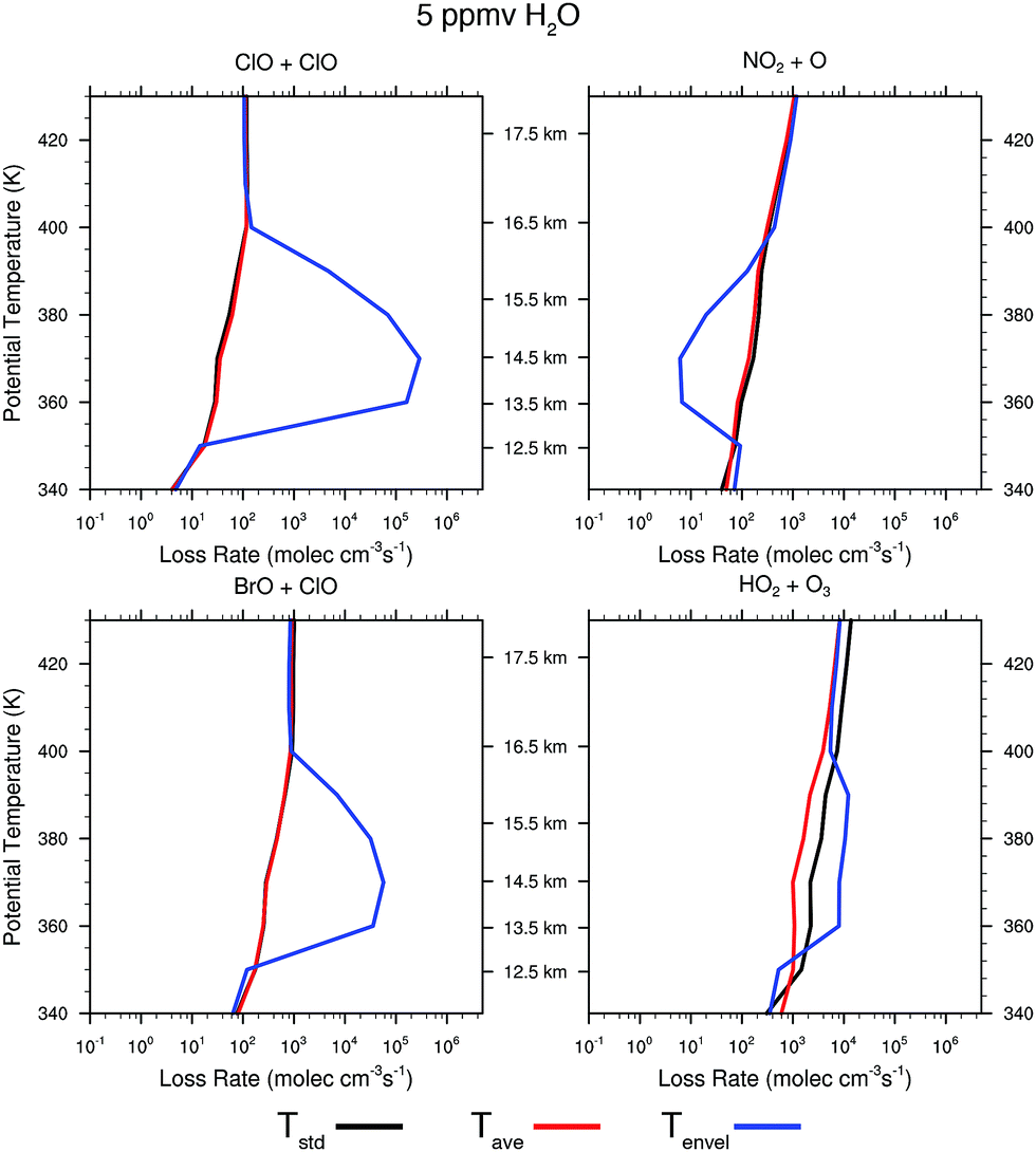 | ||
| Fig. 11 The rate of ozone loss for the four major catalytic cycles rate limited by ClO + ClO, ClO + BrO, NO2 + O, and HO2 + O3 are displayed for three different temperature profiles. The black line corresponds to the ozone loss rate for the temperature distribution Tstd as displayed in Fig. 10; the red line corresponds to the temperature Tavg; and the blue line to the temperature distribution Tenv. | ||
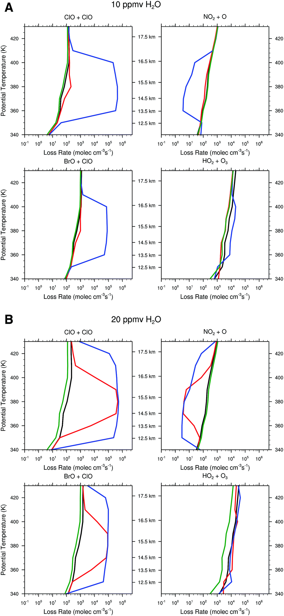 | ||
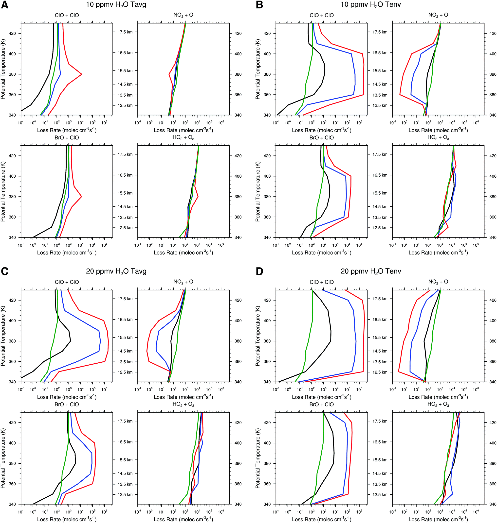
| Fig. 12 Panel A displays the ozone loss rate for the four catalytic cycles rate limited by ClO + ClO, ClO + BrO, NO2 + O, and HO2 + O3 for the case of 10 ppmv of H2O convectively injected into the stratosphere for the three temperature distributions Tstd, Tavg and Tenv; all with the HCl distribution [HCl]mid. Panel B displays the ozone loss rate for the same four catalytic cycles but for 20 ppmv H2O with the three temperature distributions Tstd, Tavg and Tenv; all with the HCl distribution [HCl]mid. In each case the reference line in green corresponds to the unperturbed case with 5 ppmv H2O and Tstd. In each case the black line corresponds to Tstd; the red line to Tavg, and the blue line to Tenv. | ||
For the case of Tstd, there is virtually no response to water vapor raised to 10 ppmv and only marginal response for 20 ppmv. For the temperature distribution represented by the observed temperature Tavg over the US in summer, the presence of convected water vapor at a mixing ratio of 10 ppmv increases the rate of ozone loss by the ClO + ClO rate limiting step only marginally, but at 20 ppmv H2O the ClO + ClO rate increases by nearly four orders of magnitude between 14 and 16 km, while increasing the ClO + BrO RLS by more than two orders of magnitude. In sharp contrast, for the observed temperature profile Tenv, at 10 ppmv the ClO + ClO RLS increases by four orders of magnitude and the ClO + BrO RLS step increases by two orders of magnitude over the significantly wider altitude range from 12 to 18 km. It is clear from comparison of panels A and B in Fig. 11 that convective injection of water vapor most significantly changes the ozone loss rate for Tavg, but that at Tenv, either 10 ppmv or 20 ppmv of convected water serves to convert a dominant fraction of inorganic chlorine to free radical form, ClO. For both 10 ppmv and 20 ppmv H2O, the HO2 + O3 RLS is essentially unaffected. The NOx catalytic cycle rate limited by NO2 + O decreases by a factor of fifty for Tenv at 10 ppmv H2O, but is unaffected at Tavg. At 20 ppmv, NO2 + O decreases by a factor of fifty for Tavg but over a more limited altitude than is the case for Tenv.
env, [HCl]mid, and [HCl]upperenv, displayed in Fig. 9 for the temperature distribution Tavg and for 10 ppmv of convectively injected water vapor. An inspection of panel A reveals that at 10 ppmv H2O and Tavg, the ClO + ClO RLS is only marginally enhanced as is the ClO + BrO RLS. But it is important to note that the HOx RLS HO2 + O3 still dominates the catalytic loss of ozone in the lower stratosphere. The NOx RLS is both largely unaffected and plays no significant quantitative role in the net O3 loss rate.
 | ||
| Fig. 13 The ozone loss as a function of altitude for combination of temperature and convectively injected water vapor are displayed in the four panels of the figure. Panel A displays the ozone loss rate for the for the four catalytic cycles rate limited by ClO + ClO, ClO + BrO, NO2 + O, and HO2 + O3 for the case of 10 ppmv H2O with the temperature distribution Tavg for the three HCl profiles [HCl]lowerenv, [HCL]mid, and [HCl]upperenv shown respectively in green, black and red. Panel B for the same conditions as panel A with Tenv in place of Tavg. Panel C is identical to the case for panel A except 20 ppmv is used rather than 10 ppmv, and panel D introduces both 20 ppmv and Tenv for the calculation defining the impact on the ozone distribution. | ||
Panel B in sharp contrast, displays a dramatic increase in the ClO + ClO RLS of some five orders of magnitude triggered by the small decrease in temperature profile between the observed temperatures of Tavg and Tenv. Inspection of panel C corresponding to 20 ppmv of convectively injected water vapor at Tavg underscores the remarkable behavior of the heterogeneous catalytic mechanism of inorganic chlorine conversion to free radical form displayed schematically in Fig. 8. Specifically, that the threshold for rapid conversion of inorganic chlorine to free radical form can be accomplished either by small decreases in temperature or by increases in the water vapor concentration. Panel D of Fig. 13, corresponding to 20 ppmv of convectively injected water vapor for the observed temperature distribution Tenv of Fig. 10, expands markedly the altitude range of accentuated ozone catalytic loss by both the ClO + ClO and ClO + BrO RLSs such that catalytic control of ozone passes from HOx control to CLOx/BrOx control and the net loss rate increases by more than two orders of magnitude.
We calculate next the impact on the ozone profile in response to the change in the rate limiting steps for the temperature profiles Tavg and Tenv in the presence of convective injection of water vapor for the range in HCl from [HCl]lowerenv, to [HCl]upperenv. Fig. 14 presents the model calculated ozone profiles for each of the temperature profiles two weeks after the convective injection of water vapor (the nominal period of time that a convectively influenced domain resides within the anti-cyclonic circulation) with water vapor elevated to 20 ppmv from 12 to 18 km. We do this for a single convective event, recognizing that on average 2000 convective events extend above approximately 16 km in a given summer. For the case of Tavg in Fig. 14 panel A, the convective injection yields a fractional reduction in ozone between 12 and 18 km of −2.5% for the [HCl]lowerenv case, but for the [HCl]upperenv case, the fractional reduction in ozone between 12 and 18 km is −34.6%. This corresponds to a decrease in the total ozone column concentration of −3.6%. As treated in Section 3, this has significant consequences for human health. Convective injection of water with the observed envelope temperature, Tenv, results in the catalytic loss rate increasing markedly over a significantly larger altitude domain such that the fractional loss of ozone over the altitude range 12 to 18 km is 67% and the fraction loss of total ozone column is 7.8% with a corresponding decrease in ozone as a function of altitude. Panel C of Fig. 14 presents a table of the fractional loss of ozone between 12 and 18 km for the cases spanning the range of observed HCl mixing ratios from [HCl]lowerenv, to [HCl]upperenv, for both the observed Tavg and Tenv for convectively injected H2O at 20 ppmv. The table also summarizes the corresponding reduction in total ozone column concentration.
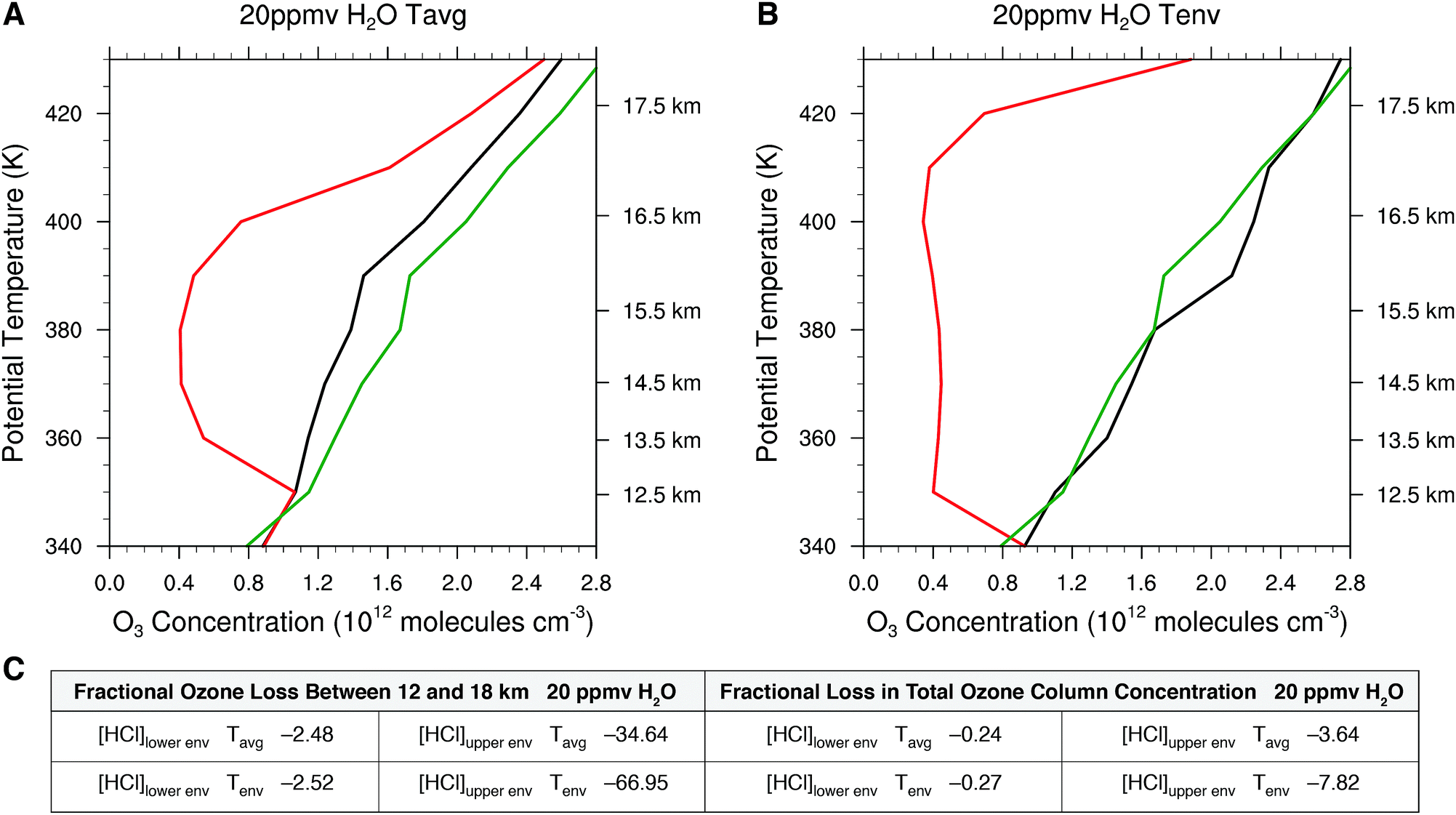 | ||
| Fig. 14 Panel A displays the impact of the sum of the rate limiting steps for the case of 20 ppmv H2O and Tavg for [HCl]lowerenv displayed in black relative to the unperturbed reference case in green and for [HCl]upperenv displayed in red. Panel B displays the same conditions as panel A except for the temperature distribution Tenv rather than Tavg. Panel C tabulates the fractional ozone loss between 12 and 18 kilometers and the fraction decrease in the total ozone column density for the temperatures Tavg and Tenv relative to the unperturbed reference case in green. | ||
3. Human health implications
A major factor underpinning the fact that the ozone shield is the most delicate aspect of habitability on the planet's surface is the fact that if the stratospheric ozone column were brought to standard temperature and pressure, that ozone column would be only ∼0.5 cm in depth. Moreover, detailed medical research has demonstrated that a 1% reduction in column ozone concentration over the US translates to a 3% increase in new skin cancer cases each year. Given that the incidence of skin cancer in the US has increased by 300% since 1992 to 3.5 million new cases a year, we can calculate the fractional increase in skin cancer incidence as a function of the percent decrease in column ozone—a result displayed in Fig. 15. This defines the accuracy with which the forecast of ozone column concentration changes must be quantitatively trusted in response to increased forcing of the climate by CO2, CH4, N2O, etc.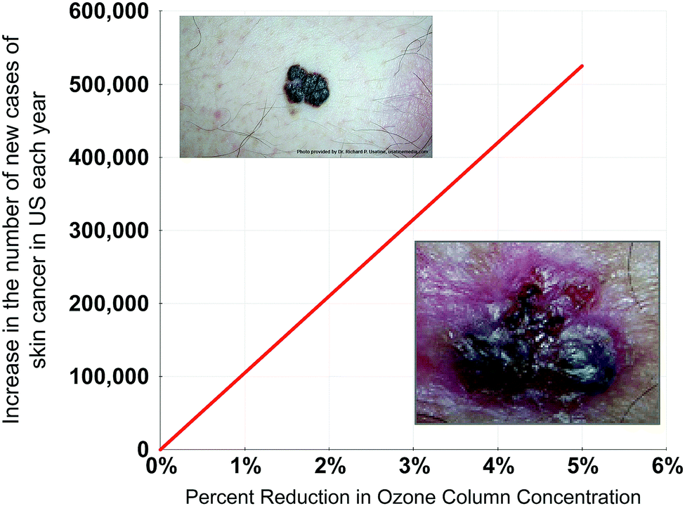 | ||
| Fig. 15 Skin cancer is primarily of two forms: melanoma displayed in the upper left, and carcinoma displayed in the lower right. Skin cancer incidence has increased 300% in the US since 1992 and now constitutes 3.5 million new cases a year. A fractional decrease in column ozone of 1% translates to a fractional increase of 3% in skin cancer incidence. This provides the information to plot the increase in the number of skin cancer cases annually vs. the percentage reduction in ozone column concentration displayed here. | ||
4. Conclusions
The discovery of deep stratospheric convective injection of water vapor over the central United States in summer was not predicted nor was the risk for ozone loss associated with convective injection incorporated into stratospheric research planning. Given the development of sophisticated data analyses employing the NEXRAD weather radar network and the availability of high spatial resolution, high accuracy in situ temperature data, what has now emerged is a new understanding of the remarkable coincidence between the conditions present in the lower stratosphere over the US in summer, and the trigger point for dramatically enhanced catalytic loss rates of ozone resulting from the temperature-water vapor kinetics of heterogeneous catalytic conversion of inorganic chlorine to free radical form on simple sulfate–water aerosols followed by the homogeneous catalytic removal of ozone by the two halogen catalytic cycles engaging the ClOOCl dimer,46 and the coupled ClO/BrO catalytic cycle.47The abrupt threshold for markedly enhanced catalytic loss of ozone as a function of temperature alone is quantitatively displayed in Fig. 11. The response of catalytic ozone loss to combinations of temperature and water vapor is displayed in Fig. 12. Finally, Fig. 13 captures the response of ozone loss rates to combinations of temperature, water vapor and available HCl—the dominant form of inorganic chlorine in the stratosphere. Of particular concern is:
(1) Warming of the surface waters of the Gulf of Mexico as a result of the increased trapping of infrared radiation by greenhouse gases fuels both the increased frequency and intensity of the convective storm systems over the Great Plains of the United States;
(2) Increased forcing of the climate by carbon dioxide and methane leads to cooling of the stratosphere—as would the loss of ozone in the critical altitude region between 14 and 18 km—thereby potentially shifting the stratosphere towards a temperature domain capable of more frequently initiated heterogeneous catalytic conversion of Cly to ClO and, in turn, increasing the rate of ozone loss;
(3) Uncertainty in forecasting the rate of increase in the intensity and frequency of severe storm systems over the central US in summer resulting from increased forcing of the climate in combination with uncertainties in the multi-decadal changes in chlorine loading of the stratosphere resulting from the global ban on CFCs and halons invoked by the Montreal Protocol;
(4) Acknowledgement of the response of the rate of ozone loss in the lower stratosphere to enhanced sulfate loading from volcanic eruptions or overt sulfate addition for climate engineering that act in concert with temperature and water vapor in controlling the rate of catalytic ozone loss;
(5) Recognition that volcanic eruptions can contain significantly elevated quantities of hydrogen halides in addition to sulfur dioxide. For example, elevated Cly was detected in the stratospheric volcanic clouds of El Chichón (1982) and Hekla (2000).76–79 From petrology, a number of historic eruptions are known to have produced large quantities of HCl and HBr, which would have exceeded peak anthropogenic Equivalent Effective Stratospheric Chlorine (EESC) that accounts for both chlorine and bromine levels, if even a small fraction of their emissions partitioned to the stratosphere.80–83 A 2016 analysis of MLS satellite observations confirms that the stratospheric injection of halogens is more frequent than previously believed;84 and
(6) Consideration of the marked sensitivity of human skin cancer incidence, in addition to increased risks to livestock and decreased staple crop production, to small increases in UV dosage levels.
Conflicts of interest
There are no conflicts to declare.Acknowledgements
This work has been supported by the National Aeronautics and Space Administration (NASA) under NASA award numbers NNX15AF60G (UV Absorption Cross Sections and Equilibrium Constant of ClOOCl Determined from New Laboratory Spectroscopy Studies of ClOOCl and ClO) and NNX15AD87G (New Laboratory Bromine Kinetics for Improving Models and Projections of Stratospheric Ozone), and a grant from the National Science Foundation (NSF) Arctic Observing Network (AON) Program under NSF award number 1203583 (Collaborative Research: Multi-Regional Scale Aircraft Observations of Methane and Carbon Dioxide Isotopic Fluxes in the Arctic).References
- J. Hansen, M. Sato, P. Hearty, R. Ruedy, M. Kelley, V. Masson-Delmotte, G. Russell, G. Tselioudis, J. Cao, E. Rignot, I. Velicogna, B. Tormey, B. Donovan, E. Kandiano, K. von Schuckmann, P. Kharecha, A. N. Legrande, M. Bauer and K.-W. Lo, Ice melt, sea level rise and superstorms: evidence from paleoclimate data, climate modeling, and modern observations that 2 °C global warming could be dangerous, Atmos. Chem. Phys., 2016, 16(6), 3761–3812 CAS.
- J. Hansen, M. Sato, G. Russell and P. Kharecha, Climate sensitivity, sea level and atmospheric carbon dioxide, Philos. Trans. R. Soc., A, 2013, 371, 20120294 CrossRef PubMed.
- D. B. Kirk-Davidoff, E. J. Hintsa, J. G. Anderson and D. W. Keith, The effect of climate change on ozone depletion through changes in stratospheric water vapour, Nature, 1999, 402, 399–401 CrossRef CAS.
- J. G. Anderson, D. K. Weisenstein, K. P. Bowman, C. R. Homeyer, J. B. Smith, D. M. Wilmouth, D. S. Sayres, J. E. Klobas, S. S. Leroy, J. A. Dykema and S. C. Wofsy, Stratospheric ozone over the United States in summer linked to observations of convection and temperature via chlorine and bromine catalysis, Proc. Natl. Acad. Sci. U. S. A., 2017, 114, E4905–E4913 CrossRef CAS PubMed.
- K. M. Walter, L. C. Smith and F. S. Chapin, Methane bubbling from northern lakes: present and future contributions to the global methane budget, Philos. Trans. R. Soc., A, 2007, 365, 1657–1676 CrossRef CAS PubMed.
- R. Commane, J. Lindaas, J. Benmergui, K. A. Luus, R. Y. Chang, B. C. Daube, E. S. Euskirchen, J. M. Henderson, A. Karion, J. B. Miller, S. M. Miller, N. C. Parazoo, J. T. Randerson, C. Sweeney, P. Tans, K. Thoning, S. Veraverbeke, C. E. Miller and S. C. Wofsy, Carbon dioxide sources from Alaska driven by increasing early winter respiration from Arctic tundra, Proc. Natl. Acad. Sci. U. S. A., 2017, 114, 5361–5366 CrossRef CAS PubMed.
- B. Buffett and D. Archer, Global inventory of methane clathrate: sensitivity to changes in the deep ocean, Earth Planet. Sci. Lett., 2004, 227, 185–199 CrossRef CAS.
- IPCC, 2007: Climate Change 2007: The Physical Science Basis, in Contribution of Working Group I to the Fourth Assessment Report of the Intergovernmental Panel on Climate Change, ed. S. Solomon, D. Qin, M. Manning, Z. Chen, M. Marquis, K. B. Averyt, M. Tignor, and H. L. Miller, Cambridge University Press, New York, 2007.
- IPCC, 2013: Climate Change 2013: The Physical Science Basis: Working Group I Contribution to the Fifth Assessment Report of the Intergovernmental Panel on Climate Change, ed. T. F. Stocker, D. Qin, G.-K. Plattner, M. Tignor, S. K. Allen, J. Boschung, A. Nauels, Y. Xia, V. Bex, and P. M. Midgley, Cambridge University Press, New York, 2013.
- E. A. Schuur, A. D. McGuire, C. Schädel, G. Grosse, J. W. Harden, D. J. Hayes, G. Hugelius, C. D. Koven, P. Kuhry, D. M. Lawrence, S. M. Natali, D. Olefeldt, V. E. Romanovsky, K. Schaefer, M. R. Turetsky, C. C. Treat and J. E. Vonk, Climate change and the permafrost carbon feedback, Nature, 2015, 520, 171–179 CrossRef CAS PubMed.
- S. A. Zimov, E. A. Schuur and F. S. Chapin, Permafrost and the global carbon budget, Science, 2006, 312, 1612–1613 CrossRef CAS PubMed.
- S. Palmer, A. Shepherd, P. Nienow and I. Joughin, Seasonal speedup of the Greenland Ice Sheet linked to routing of surface water, Earth Planet. Sci. Lett., 2011, 302, 423–428 CrossRef CAS.
- I. Velicogna, Increasing rates of ice mass loss from the Greenland and Antarctic ice sheets revealed by GRACE, Geophys. Res. Lett., 2009, 36, L19503 CrossRef.
- A. Dutton, A. E. Carlson, A. J. Long, G. A. Milne, P. U. Clark, R. DeConto, B. P. Horton, S. Rahmstorf and M. E. Raymo, Sea-level rise due to polar ice-sheet mass loss during past warm periods, Science, 2015, 349, aaa4019 CrossRef CAS PubMed.
- M. E. Raymo and J. X. Mitrovica, Collapse of polar ice sheets during the stage 11 interglacial, Nature, 2012, 483, 453–456 CrossRef CAS PubMed.
- T. F. Hanisco, E. J. Moyer, E. M. Weinstock, J. M. St. Clair, D. S. Sayres, J. B. Smith, R. Lockwood, J. G. Anderson, A. E. Dessler, F. N. Keutsch, J. R. Spackman, W. G. Read and T. P. Bui, Observations of deep convective influence on stratospheric water vapor and its isotopic composition, Geophys. Res. Lett., 2007, 34, L04814 CrossRef.
- J. G. Anderson, D. M. Wilmouth, J. B. Smith and D. S. Sayres, UV dosage levels in summer: increased risk of ozone loss from convectively injected water vapor, Science, 2012, 337, 835–839 CrossRef CAS PubMed.
- C. R. Homeyer, L. L. Pan and M. C. Barth, Transport from convective overshooting of the extratropical tropopause and the role of large-scale lower stratosphere stability, J. Geophys. Res.: Atmos., 2014, 119, 2220–2240 Search PubMed.
- L. L. Pan, E. L. Atlas, R. J. Salawitch, S. B. Honomichl, J. F. Bresch, W. J. Randel, E. C. Apel, R. S. Hornbrook, A. J. Weinheimer, D. C. Anderson, S. J. Andrews, S. Baidar, S. P. Beaton, T. L. Campos, L. J. Carpenter, D. Chen, B. Dix, V. Donets, S. R. Hall, T. F. Hanisco, C. R. Homeyer, L. G. Huey, J. B. Jensen, L. Kaser, D. E. Kinnison, T. K. Koenig, J.-F. Lamarque, C. Liu, J. Luo, Z. J. Luo, D. D. Montzka, J. M. Nicely, R. B. Pierce, D. D. Riemer, T. Robinson, P. Romashkin, A. Saiz-Lopez, S. Schauffler, O. Shieh, M. H. Stell, K. Ullmann, G. Vaughan, R. Volkamer and G. Wolfe, The Convective Transport of Active Species in the Tropics (CONTRAST) Experiment, Bull. Am. Meteorol. Soc., 2017, 98, 106–128 CrossRef.
- A. E. Gill, Some simple solutions for heat-induced tropical circulation, Q. J. R. Meteorol. Soc., 1980, 106, 447–462 CrossRef.
- E. M. Weinstock, J. V. Pittman, D. S. Sayres, J. B. Smith, J. G. Anderson, S. C. Wofsy, I. Xueref, C. Gerbig, B. C. Daube, L. Pfister, E. C. Richard, B. A. Ridley, A. J. Weinheimer, H.-J. Jost, J. P. Lopez, M. Loewenstein and T. L. Thompson, Quantifying the impact of the North American monsoon and deep midlatitude convection on the subtropical lowermost stratosphere using in situ measurements, J. Geophys. Res., 2007, 112, D18310 CrossRef.
- S. Solomon, Stratospheric ozone depletion: A review of concepts and history, Rev. Geophys., 1999, 37, 275–316 CrossRef CAS.
- D. W. Fahey, S. R. Kawa, E. L. Woodbridge, P. Tin, J. C. Wilson, H. H. Jonsson, J. E. Dye, D. Baumgardner, S. Borrmann, D. W. Toohey, L. M. Avallone, M. H. Proffitt, J. Margitan, M. Loewenstein, J. R. Podolske, R. J. Salawitch, S. C. Wofsy, M. K. W. Ko, D. E. Anderson, M. R. Schoeber and K. R. Chan, In situ measurements constraining the role of sulphate aerosols in mid-latitude ozone depletion, Nature, 1993, 363, 509–514 CrossRef CAS.
- R. J. Salawitch, D. K. Weisenstein, L. J. Kovalenko, C. E. Sioris, P. O. Wennberg, K. Chance, M. K. W. Ko and C. A. McLinden, Sensitivity of ozone to bromine in the lower stratosphere, Geophys. Res. Lett., 2005, 32, L05811 CrossRef.
- S. Solomon, R. W. Portmann, R. R. Garcia, W. Randel, F. Wu, R. Nagatani, J. Gleason, L. Thomason, L. R. Poole and M. P. McCormick, Ozone depletion at mid-latitudes: coupling of volcanic aerosols and temperature variability to anthropogenic chlorine, Geophys. Res. Lett., 1998, 25, 1871–1874 CrossRef CAS.
- T. Canty, N. R. Mascioli, M. D. Smarte and R. J. Salawitch, An empirical model of global climate – part 1: a critical evaluation of volcanic cooling, Atmos. Chem. Phys., 2013, 13, 3997–4031 Search PubMed.
- S. Tilmes, R. R. Garcia, D. E. Kinnison, A. Gettelman and P. J. Rasch, Impact of geoengineered aerosols on the troposphere and stratosphere, J. Geophys. Res., 2009, 114, D12305 CrossRef.
- C. G. McCormack, W. Born, P. J. Irvine, E. P. Achterberg, T. Amano, J. Ardron, P. N. Foster, J.-P. Gattuso, S. J. Hawkins, E. Hendy, W. D. Kissling, S. E. Lluch-Cota, E. J. Murphy, N. Ostle, N. J. P. Owens, R. I. Perry, H. O. Pörtner, R. J. Scholes, F. M. Schurr, O. Schweiger, J. Settele, R. K. Smith, S. Smith, J. Thompson, D. P. Tittensor, M. van Kleunen, C. Vivian, K. Vohland, R. Warren, A. R. Watkinson, S. Widdicombe, P. Williamson, E. Woods, J. J. Blackstock and W. J. Sutherland, Key impacts of climate engineering on biodiversity and ecosystems, with priorities for future research, J. Integr. Environ. Sci., 2016, 13, 103–128 Search PubMed.
- P. J. Crutzen, Albedo Enhancement by Stratospheric Sulfur Injections: A Contribution to Resolve a Policy Dilemma?, Clim. Change, 2006, 77, 211–220 CrossRef CAS.
- G. Pitari, V. Aquila, B. Kravitz, A. Robock, S. Watanabe, I. Cionni, N. D. Luca, G. D. Genova, E. Mancini and S. Tilmes, Stratospheric ozone response to sulfate geoengineering: results from the geoengineering Model Intercomparison Project (GeoMIP), J. Geophys. Res.: Atmos., 2014, 119, 2629–2653 CAS.
- J. A. Dykema, D. W. Keith, J. G. Anderson and D. Weisenstein, Stratospheric controlled perturbation experiment: a small-scale experiment to improve understanding of the risks of solar geoengineering, Philos. Trans. R. Soc., A, 2014, 372, 20140059 CrossRef PubMed.
- D. K. Weisenstein, D. W. Keith and J. A. Dykema, Solar geoengineering using solid aerosol in the stratosphere, Atmos. Chem. Phys., 2015, 15, 11835–11859 CrossRef CAS.
- Z. Feng, L. R. Leung, S. Hagos, R. A. Houze, C. D. Burleyson and K. Balaguru, More frequent intense and long-lived storms dominate the springtime trend in central US rainfall, Nat. Commun., 2016, 7, 13429 CrossRef CAS PubMed.
- M. K. Tippett, C. Lepore and J. E. Cohen, More tornadoes in the most extreme U.S. tornado outbreaks, Science, 2016, 354, 1419–1423 CrossRef CAS PubMed.
- N. S. Diffenbaugh, M. Scherer and R. J. Trapp, Robust increases in severe thunderstorm environments in response to greenhouse forcing, Proc. Natl. Acad. Sci. U. S. A., 2013, 110, 16361–16366 CrossRef CAS PubMed.
- R. J. Trapp and K. A. Hoogewind, The realization of extreme tornadic storm events under future anthropogenic climate change, J. Clim., 2016, 29, 5251–5265 CrossRef.
- D. K. Weisenstein, G. K. Yue, M. K. W. Ko, N.-D. Sze, J. M. Rodriguez and C. J. Scott, A two-dimensional model of sulfur species and aerosols, J. Geophys. Res., 1997, 102, 13019–13035 CrossRef CAS.
- M. K. W. Ko, N.-D. Sze, C. J. Scott and D. K. Weisenstein, On the relation between stratospheric chlorine/bromine loading and short-lived tropospheric source gases, J. Geophys. Res., 1997, 102, 25507–25517 CrossRef CAS.
- C. P. Rinsland, D. K. Weisenstein, M. K. W. Ko, C. J. Scott, L. S. Chiou, E. Mahieu, R. Zander and P. Demoulin, Post-Mount Pinatubo eruption ground-based infrared stratospheric column measurements of HNO3, NO, and NO2 and their comparison with model calculations, J. Geophys. Res., 2003, 108, 4437 CrossRef.
- M. A. Weinstock, Overview of ultraviolet radiation and cancer: what is the link? How are we doing?, Environ. Health Perspect., 1995, 103, 251–254 CrossRef PubMed.
- T. L. Diepgen and V. Mahler, The epidemiology of skin cancer, Br. J. Dermatol., 2002, 146, 1–6 CrossRef PubMed.
- Y. Matsumura and H. N. Ananthaswamy, Toxic effects of ultraviolet radiation on the skin, Toxicol. Appl. Pharmacol., 2004, 195, 298–308 CrossRef CAS PubMed.
- M. Tevini and A. H. Teramura, UV-B effects on terrestrial plants, Photochem. Photobiol., 1989, 50, 479–487 CrossRef CAS.
- M. J. Molina and F. S. Rowland, Stratospheric sink for chlorofluoromethanes: chlorine atom-catalysed destruction of ozone, Nature, 1974, 249, 810–812 CrossRef CAS.
- S. Solomon, R. R. Garcia, F. S. Rowland and D. J. Wuebbles, On the depletion of Antarctic ozone, Nature, 1986, 321, 755–758 CrossRef CAS.
- L. T. Molina and M. J. Molina, Production of chlorine oxide (Cl2O2) from the self-reaction of the chlorine oxide (ClO) radical, J. Phys. Chem., 1987, 91, 433–436 CrossRef CAS.
- M. B. McElroy, R. J. Salawitch, S. C. Wofsy and J. A. Logan, Reductions of Antarctic ozone due to synergistic interactions of chlorine and bromine, Nature, 1986, 321, 759–762 CrossRef CAS.
- J. G. Anderson, W. H. Brune and D. W. Toohey, Free radicals within the Antarctic vortex: the role of CFCs in Antarctic ozone loss, Science, 1991, 251, 39–46 CAS.
- W. H. Brune, D. W. Toohey, J. G. Anderson and K. R. Chan, In situ observations of ClO in the Arctic stratosphere: ER-2 aircraft results from 59°N to 80°N latitude, Geophys. Res. Lett., 1990, 17, 505–508 CrossRef.
- R. M. Stimpfle, R. C. Cohen, G. P. Bonne, P. B. Voss, K. K. Perkins, L. C. Koch, J. G. Anderson, R. J. Salawitch, S. A. Lloyd, R. S. Gao, L. A. Del Negro, E. R. Keim and T. P. Bui, The coupling of ClONO2, ClO, and NO2 in the lower stratosphere from in situ observations using the NASA ER-2 aircraft, J. Geophys. Res., 1999, 104, 26705–26714 CrossRef CAS.
- P. A. Newman, N. R. Harris, A. Adriani, G. T. Amanatidis, J. G. Anderson, G. O. Braathen, W. H. Brune, K. S. Carslaw, M. S. Craig, P. L. DeCola, M. Guirlet, R. S. Hipskind, M. J. Kurylo, H. Küllmann, N. Larsen, G. J. Mégie, J.-P. Pommereau, L. R. Poole, M. R. Schoeberl, F. Stroh, O. B. Toon, C. R. Trepte and M. Van Roozendael, An overview of the SOLVE/THESEO 2000 campaign, J. Geophys. Res., 2002, 107, 8259 CrossRef.
- T. F. Hanisco, J. B. Smith, R. M. Stimpfle, D. M. Wilmouth, K. K. Perkins, J. R. Spackman, J. G. Anderson, D. Baumgardner, B. Gandrud, C. R. Webster, S. Dhaniyala, K. A. McKinney and T. P. Bui, Quantifying the rate of heterogeneous processing in the Arctic polar vortex with in situ observations of OH, J. Geophys. Res., 2002, 107, 8278 CrossRef.
- R. M. Stimpfle, D. M. Wilmouth, R. J. Salawitch and J. G. Anderson, First measurements of ClOOCl in the stratosphere: the coupling of ClOOCl and ClO in the Arctic polar vortex, J. Geophys. Res., 2004, 109, D03301 CrossRef.
- D. M. Wilmouth, R. M. Stimpfle, J. G. Anderson, J. W. Elkins, D. F. Hurst, R. J. Salawitch and L. R. Lait, Evolution of inorganic chlorine partitioning in the Arctic polar vortex, J. Geophys. Res., 2006, 111, D16308 CrossRef.
- G. L. Manney, M. L. Santee, M. Rex, N. J. Livesey, M. C. Pitts, P. Veefkind, E. R. Nash, I. Wohltmann, R. Lehmann, L. Froidevaux, L. R. Poole, M. R. Schoeberl, D. P. Haffner, J. Davies, V. Dorokhov, H. Gernandt, B. Johnson, R. Kivi, E. Kyrö, N. Larsen, P. F. Levelt, A. Makshtas, C. T. McElroy, H. Nakajima, M. C. Parrondo, D. W. Tarasick, P. von der Gathen, K. A. Walker and N. S. Zinoviev, Unprecedented Arctic ozone loss in 2011, Nature, 2011, 478, 469–475 CrossRef CAS PubMed.
- S. Solomon, R. W. Portmann, R. R. Garcia, L. W. Thomason, L. R. Poole and M. P. McCormick, The role of aerosol variations in anthropogenic ozone depletion at northern midlatitudes, J. Geophys. Res., 1996, 101, 6713–6727 CrossRef CAS.
- Q. Shi, J. T. Jayne, C. E. Kolb, D. R. Worsnop and P. Davidovits, Kinetic model for reaction of ClONO2 with H2O and HCl and HOCl with HCl in sulfuric acid solutions, J. Geophys. Res., 2001, 106, 24259–24274 CrossRef CAS.
- K. Drdla, Temperature thresholds for polar stratospheric ozone, Trans., Am. Geophys. Union, 2005, 86 Search PubMed , Abstract A31D-03.
- K. Drdla and R. Müller, Temperature thresholds for chlorine activation and ozone loss in the polar stratosphere, Ann. Geophys., 2012, 30, 1055–1073 CrossRef CAS.
- J. B. Burkholder, S. P. Sander, J. Abbatt, J. R. Barker, R. E. Huie, C. E. Kolb, M. J. Kurylo, V. L. Orkin, D. M. Wilmouth and P. H. Wine, Chemical Kinetics and Photochemical Data for Use in Atmospheric Studies, Evaluation No. 18, JPL Publication 15-10, Jet Propulsion Laboratory, Pasadena, 2015 Search PubMed.
- P. O. Wennberg, R. C. Cohen, R. M. Stimpfle, J. P. Koplow, J. G. Anderson, R. J. Salawitch, D. W. Fahey, E. L. Woodbridge, E. R. Keim, R. S. Gao, C. R. Webster, R. D. May, D. W. Toohey, L. M. Avallone, M. H. Proffitt, M. Loewenstein, J. R. Podolske, K. R. Chan and S. C. Wofsy, Removal of stratospheric O3 by radicals: in situ measurements of OH, HO2, NO, NO2, ClO, and BrO, Science, 1994, 266, 398–404 CAS.
- D. L. Solomon, K. P. Bowman and C. R. Homeyer, Tropopause-penetrating convection from three-dimensional gridded NEXRAD data, J. Appl. Meteor. Climatol., 2016, 55, 465–478 CrossRef.
- O. B. Toon, H. Maring, J. Dibb, R. Ferrare, D. J. Jacob, E. J. Jensen, Z. J. Luo, G. G. Mace, L. L. Pan, L. Pfister, K. H. Rosenlof, J. Redemann, J. S. Reid, H. B. Singh, A. M. Thompson, R. Yokelson, P. Minnis, G. Chen, K. W. Jucks and A. Pszenny, Planning, implementation, and scientific goals of the studies of emissions and atmospheric composition, clouds and climate coupling by regional surveys (SEAC4RS) field mission: planning SEAC4RS, J. Geophys. Res.: Atmos., 2016, 121, 4967–5009 CAS.
- C. R. Homeyer and M. R. Kumjian, Microphysical characteristics of overshooting convection from polarimetric radar observations, J. Atmos. Sci., 2015, 72, 870–891 CrossRef.
- T. P. Marcy, D. W. Fahey, R. S. Gao, P. J. Popp, E. C. Richard, T. L. Thompson, K. H. Rosenlof, E. A. Ray, R. J. Salawitch, C. S. Atherton, D. J. Bergmann, B. A. Ridley, A. J. Weinheimer, M. Loewenstein, E. M. Weinstock and M. J. Mahoney, Quantifying stratospheric ozone in the upper troposphere with in situ measurements of HCl, Science, 2004, 304, 261 CrossRef CAS PubMed.
- M. J. Schwartz, W. G. Read, M. L. Santee, N. J. Livesey, L. Froidevaux, A. Lambert and G. L. Manney, Convectively injected water vapor in the North American summer lowermost stratosphere, Geophys. Res. Lett., 2013, 40, 2316–2321 CrossRef.
- W. J. Randel, E. Moyer, M. Park, E. Jensen, P. Bernath, K. Walker and C. Boone, Global variations of HDO and HDO/H2O ratios in the upper troposphere and lower stratosphere derived from ACE-FTS satellite measurements, J. Geophys. Res., 2012, 117, D06303 CrossRef.
- D. S. Sayres, L. Pfister, T. F. Hanisco, E. J. Moyer, J. B. Smith, J. M. St. Clair, A. S. O’Brien, M. F. Witinski, M. Legg and J. G. Anderson, Influence of convection on the water isotopic composition of the tropical tropopause layer and tropical stratosphere, J. Geophys. Res., 2010, 115, D00J20 CrossRef.
- M. J. Alexander, J. Gille, C. Cavanaugh, M. Coffey, C. Craig, T. Eden, G. Francis, C. Halvorson, J. Hannigan, R. Khosravi, D. Kinnison, H. Lee, S. Massie, B. Nardi, J. Barnett, C. Hepplewhite, A. Lambert and V. Dean, Global estimates of gravity wave momentum flux from high resolution dynamics limb sounder observations, J. Geophys. Res., 2008, 113, D15S18 CrossRef.
- A. C. Maycock, K. P. Shine and M. M. Joshi, The temperature response to stratospheric water vapour changes, Q. J. R. Meteorol. Soc., 2011, 137, 1070–1082 CrossRef.
- J. A. Dykema, D. W. Keith and F. N. Keutsch, Improved aerosol radiative properties as a foundation for solar geoengineering risk assessment, Geophys. Res. Lett., 2016, 43, 7758–7766 CrossRef CAS.
- T. R. Koby, PhD thesis, Development of a trajectory model for the analysis of stratospheric water vapor, Harvard Univ, Cambridge, MA, 2016 Search PubMed.
- A. E. Dessler and S. C. Sherwood, Effect of convection on the summertime extratropical lower stratosphere, J. Geophys. Res., 2004, 109, D23301 CrossRef.
- Y. Sun and Y. Huang, An examination of convective moistening of the lower stratosphere using satellite data, Earth Space Sci., 2015, 2, 320–330 CrossRef.
- W. J. Randel, K. Zhang and R. Fu, What controls stratospheric water vapor in the NH summer monsoon regions?, J. Geophys. Res.: Atmos., 2015, 120, 7988–8001 Search PubMed.
- D. E. Hunton, A. A. Viggiano, T. M. Miller, J. O. Ballenthin, J. M. Reeves, J. C. Wilson, S.-H. Lee, B. E. Anderson, W. H. Brune, H. Harder, J. B. Simpas and N. Oskarsson, In situ aircraft observations of the 2000 Mt. Hekla volcanic cloud: composition and chemical evolution in the Arctic lower stratosphere, J. Volcanol. Geotherm. Res., 2005, 145, 23–34 CrossRef CAS.
- W. I. Rose, G. A. Millard, T. A. Mather, D. E. Hunton, B. Anderson, C. Oppenheimer, B. F. Thornton, T. M. Gerlach, A. A. Viggiano, Y. Kondo, T. M. Miller and J. O. Ballenthin, Atmospheric chemistry of a 33–34 hour old volcanic cloud from Hekla Volcano (Iceland): insights from direct sampling and the application of chemical box modeling, J. Geophys. Res., 2006, 111, D20206 CrossRef.
- G. A. Millard, T. A. Mather, D. M. Pyle, W. I. Rose and B. Thornton, Halogen emissions from a small volcanic eruption: modeling the peak concentrations, dispersion, and volcanically induced ozone loss in the stratosphere, Geophys. Res. Lett., 2006, 33, L19815 CrossRef.
- W. G. Mankin and M. T. Coffey, Increased stratospheric hydrogen chloride in the El Chichon cloud, Science, 1984, 226, 170–172 CAS.
- A. Cadoux, B. Scaillet, S. Bekki, C. Oppenheimer and T. H. Druitt, Stratospheric Ozone destruction by the Bronze-Age Minoan eruption (Santorini Volcano, Greece), Sci. Rep., 2015, 5, 12243 CrossRef CAS PubMed.
- C. M. Vidal, N. Métrich, J.-C. Komorowski, I. Pratomo, A. Michel, N. Kartadinata, V. Robert and F. Lavigne, The 1257 Samalas eruption (Lombok, Indonesia): the single greatest stratospheric gas release of the Common Era, Sci. Rep., 2016, 6, 34868 CrossRef CAS PubMed.
- S. Kutterolf, T. H. Hansteen, A. Freundt, H. Wehrmann, K. Appel, K. Krüger and W. Pérez, Bromine and chlorine emissions from Plinian eruptions along the Central American Volcanic Arc: from source to atmosphere, Earth Planet. Sci. Lett., 2015, 429, 234–246 CrossRef CAS.
- S. Kutterolf, T. H. Hansteen, K. Appel, A. Freundt, K. Kruger, W. Perez and H. Wehrmann, Combined bromine and chlorine release from large explosive volcanic eruptions: a threat to stratospheric ozone?, Geology, 2013, 41, 707–710 CrossRef CAS.
- S. A. Carn, L. Clarisse and A. J. Prata, Multi-decadal satellite measurements of global volcanic degassing, J. Volcanol. Geotherm. Res., 2016, 311, 99–134 CrossRef CAS.
| This journal is © the Owner Societies 2018 |