DOI:
10.1039/C6SM00697C
(Paper)
Soft Matter, 2017,
13, 196-211
Dynamics of a microorganism in a sheared viscoelastic liquid
Received
22nd March 2016
, Accepted 30th June 2016
First published on 4th July 2016
Abstract
In this paper, we investigate the dynamics of a model spherical microorganism, called squirmer, suspended in a viscoelastic fluid undergoing unconfined shear flow. The effect of the interplay of shear flow, fluid viscoelasticity, and self-propulsion on the orientational dynamics is addressed. In the limit of weak viscoelasticity, quantified by the Deborah number, an analytical expression for the squirmer angular velocity is derived by means of the generalized reciprocity theorem. Direct finite element simulations are carried out to study the squirmer dynamics at larger Deborah numbers. Our results show that the orientational dynamics of active microorganisms in a sheared viscoelastic fluid greatly differs from that observed in Newtonian suspensions. Fluid viscoelasticity leads to a drift of the particle orientation vector towards the vorticity axis or the flow-gradient plane depending on the Deborah number, the relative weight between the self-propulsion velocity and the flow characteristic velocity, and the type of swimming. Generally, pullers and pushers show an opposite equilibrium orientation. The results reported in the present paper could be helpful in designing devices where separation of microorganisms, based on their self-propulsion mechanism, is obtained.
1 Introduction
Suspensions of swimming microorganisms have excited much interest over the last few decades due to their importance in medicine,1 ecology,2 and in technological applications.3 As a matter of fact, the hydrodynamics of active suspensions is central in many recent fundamental studies.4–6
Much effort, indeed, has been devoted to understanding the propulsion mechanism of single organisms or the collective dynamics of self-propelling particles through a Newtonian medium under quiescent conditions.7–11 Interesting phenomena, however, have been observed when active suspensions are subjected to external flows. For instance, experiments12,13 and simulations14 have shown that spermatozoa experience the so-called rheotaxis, that is, the tendency of swimming upstream when subjected to external flows. Active stresses generated by swimming microorganisms also significantly impact the rheology of the suspension.15,16
In many situations of interest, small organisms swim through biological fluids such as mucus which display highly viscoelastic properties.17 The effect of a quiescent viscoelastic fluid on the locomotion of microorganisms has recently received much attention in the literature and a comprehensive review on the topic can be found in a recent book chapter.18 Most of the works have investigated the effect of viscoelasticity on the swimming velocity and efficiency of active particles19–23 or the dynamics of ciliated organisms close to boundaries.24–26 Much less is, instead, known when an external flow is applied. In this regard, we are aware of only two recent works where the dynamics of active microorganisms suspended in a viscoelastic fluid undergoing vortical27 and Poiseuille flow28 is investigated. In both works, the suspending medium is modelled by the so-called second-order fluid (SOF) constitutive equation which is valid for slow and slowly varying flow conditions. Nevertheless, interesting phenomena such as the emergence of well-defined patterns in vortical flow27 and an increasing tendency of swimming upstream in Poiseuille flow28 have been reported.
As the characteristic flow rates increase, viscoelastic effects become relevant and more complex microorganism dynamics are expected. The dramatic effect of fluid viscoelasticity is already evident in passive suspensions where peculiar phenomena occur as compared to the Newtonian case.29 Of course, the addition of a self-propulsion velocity would even more complicate the dynamics of the suspended particles.
The aim of the present work is to investigate the effect of the complex interplay between the swimming mechanism, viscoelasticity and an external flow field on the dynamics of microorganisms. Specifically, we present a detailed study on the dynamics of a spherical ciliated microorganism suspended in a viscoelastic fluid undergoing unbounded shear flow. We first perform a perturbative analysis at small Deborah numbers (defined as the product between the fluid relaxation time and the applied shear rate), for which the rotational velocity of the microorganism can be analytically computed. Numerical simulations are, then, carried out to investigate the particle dynamics at high Deborah numbers.
The present work is organized as follows: in Section 2, we present the model we used for the microswimmer; the equations governing the problem under investigation are reported in Section 3; the numerical method is briefly discussed in Section 4; in Sections 5 and 6, the results obtained from the perturbative analysis (low Deborah numbers) and numerical simulations (high Deborah numbers) are presented, respectively; and finally, conclusions are drawn in Section 7.
2 Microorganism model
One of the most common mechanisms exploited by microorganisms for generating propulsion is the undulatory movement of many small flagella, called cilia, positioned on the organism surface. Examples of these ciliated microorganisms are Paramecium, Volvox, and Opalina. The prediction of the locomotion of a microorganism through an accurate modeling of the beating of a large number of cilia on its surface is extremely difficult. It is intuitive, indeed, that an accurate description of the motion of all the flexible cilia is not feasible, especially if one is interested in the dynamics of the entire microorganism and not in the dynamics of a single cilium. To overcome this difficulty, different simplifying models have been proposed that take into account the motion of many cilia on the microorganism surface (or even an actual surface distortion). In this work, we choose the model introduced for the first time by Lighthill30 and Blake,31 and widely used in the literature.32–36 In this model, actual cilia motions are replaced by a steady tangential ‘slip velocity’ on a rigid boundary representing the microorganism surface. The slip velocity is, in fact, a greatly simplified modeling of the time-averaged ciliary propulsion.37 In the rest of the paper, we will refer to this model microorganism as a ‘squirmer’.
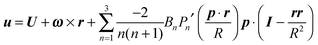
In the context of the Lighthill–Blake model, we consider the squirmer as a sphere of radius R propelling along a direction denoted by an orientation vector p through axisymmetric and time-independent surface tangential velocities. The velocity on the surface of the squirmer is given by
| | 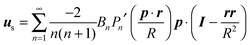 | (1) |
where
Pn′ is the derivative of the
nth Legendre polynomial with respect to its argument and
r is the position vector of a point on the squirmer surface computed from its center of volume. In the present work, we consider
Bn = 0 for
n > 3. Thus, the specification of the coefficients
B1,
B2, and
B3 completely determines the type of swimming. Although almost all the previous works on a similar subject limit the expansion to
n = 2, we investigate also the effect of
B3 in view of the recent results on the relevance of higher modes to the swimming of microorganisms in shear-thinning fluids.
38 A squirmer with a positive ratio

is called puller, as its maximum tangential velocity is on the frontal hemisphere; in other words, a puller generates propulsion from the front. Squirmers with a negative ratio

are called pushers, as they generate propulsion from the rear. When
B2 = 0, the organism is called neutral. The
B3 mode is responsible for a force quadrupole in the fluid and can be used to model fore–aft symmetric differences in cilia beating. In a quiescent Newtonian fluid, the translational velocity of the squirmer is simply equal to

as shown in the original paper of Blake.
31 Note that a squirmer has no self-induced rotational velocity as the slip velocity in
eqn (1) through which the microorganism propels is axisymmetric.
We emphasize that, in view of the explicit time dependency of the viscoelastic stress constitutive equation, a steady (rather than a time-dependent) boundary condition on the squirmer surface may not capture all of the features of a real microorganism that swims in a sheared viscoelastic fluid. On the other hand, we believe that the simple steady slip velocity adopted in the present work allows one to understand the main characteristics of the microorganism dynamics when an external shear flow is coupled with self-propulsion and viscoelasticity, with a relatively small number of parameters to model the swimming velocity. (Notice that a time-dependent slip velocity would add at least one frequency for each mode and a shift angle.) Of course, the approximation of using a steady model is more and more accurate if the (long) time scale over which the orientation and position of the squirmer evolve is well-separated from the (short) time scale of the boundary actuation.
3 Governing equations
In this work, we study the dynamics of a spherical microorganism of radius R suspended in a viscoelastic fluid undergoing an unbounded shear flow. The system under investigation is schematically depicted in Fig. 1. We assume that the distance H between the walls and the distance between the particle and the walls are much larger than the microorganism radius R. A Cartesian reference frame is selected with x, y and z the directions of flow, gradient and vorticity, respectively; with this choice, the undisturbed flow field far from the squirmer is u∞ = (ux,∞, uy,∞, uz,∞) = (![[small gamma, Greek, dot above]](https://www.rsc.org/images/entities/i_char_e0a2.gif) y, 0, 0), where is the shear rate. The microorganism swimming direction is denoted by the vector p.
y, 0, 0), where is the shear rate. The microorganism swimming direction is denoted by the vector p.
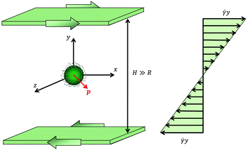 |
| | Fig. 1 Schematic picture of the problem investigated in this work. A spherical microorganism of radius R is swimming in the direction denoted by the vector p (in red), while the fluid is subjected to a shear flow. The undisturbed (i.e., without the microorganism) velocity profile is shown on the right. | |
In the low-Reynolds number regime, the equations describing the fluid motion are the continuity and the momentum balance equations:
with
u the fluid velocity and
Σ the total stress tensor:
| | | Σ = −pI + ηs(∇u + ∇uT) + τ | (4) |
In
eqn (4),
p is the pressure,
I is the unity tensor,
ηs is the viscosity of a Newtonian solvent, and
τ is the viscoelastic stress tensor, for which a constitutive equation has to be specified. In the present work, we consider the Giesekus model as the constitutive equation for the viscoelastic stress tensor, which is a good model for many dilute and semi-dilute polymer solutions:
39| | 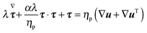 | (5) |
In the above equation,
ηp is the polymer viscosity,
λ the fluid relaxation time, and the dimensionless parameter
α is the so-called ‘mobility parameter’. For
α = 0, the Giesekus model reduces to the upper-convected Maxwell model
39 that predicts a viscosity constant with the shear rate and a non-zero first normal stress difference
N1 =
Σxx −
Σyy. For
α > 0, the Giesekus model predicts shear-thinning (
i.e., decreasing viscosity with increasing shear rate), a non-zero first and second normal stress difference
N2 =
Σyy −
Σzz. The symbol (∇) in
eqn (5) denotes the upper-convected time derivative defined as
| | 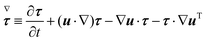 | (6) |
The boundary condition far from the swimmer is given by
with
u∞ the externally imposed shear flow. Furthermore, the boundary condition at the surface of the microorganism is given by
| |  | (8) |
where
U and
ω are the translational and rotational velocities of the swimmer (to be determined), and
r =
x −
X with
x the position vector of a point of the spherical surface and
X the position vector of the particle centroid.
To close the hydrodynamic problem, we need to consider the force and torque balances on the squirmer surface. Assuming negligible inertia, the squirmer is force- and torque-free:
| | 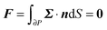 | (9) |
| | 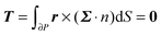 | (10) |
with
n the outwardly directed unit normal vector to the particle boundary. Notice that, for a spherical particle,
n =
r/
R.
Finally, an initial condition for τ is required. We assume a stress-free condition, i.e., that the stress is zero everywhere in the fluid at the initial time: τ|t=0 = 0.
The solution of the just presented equations gives the time evolution of the fields u, p, and τ as well as the time evolution of the microorganism rotational velocity ω and of the swimming velocity U. Once the translational and rotational velocities have been computed, the evolution of the swimmer centroid and orientation vector can be readily calculated from the following kinematic equations:
| | | ṗ(t) = ω × p(t), p|t=0 = p0 | (12) |
where
X0 and
p0 are the initial particle position and orientation. Notice that, since we consider an unbounded domain, the evolution of the particle center of volume does not affect the particle kinematic quantities,
i.e., at any position within the domain, the squirmer always ‘feels’ the same shear flow field.
It is convenient to make the above equation dimensionless. We select the inverse of the imposed shear rate −1 as the characteristic time, the radius R of the swimmer as the characteristic length, and η0 as the characteristic stress, where η0 = ηs + ηp is the zero-shear viscosity. By using these characteristic quantities, the governing equations in dimensionless form can be readily obtained. The continuity and the momentum balances are
The total stress tensor is expressed as
| | | Σ* = −p*I + (1 − ηr)(∇u* + ∇u*T) + τ* | (15) |
and the constitutive equation is given by
| |  | (16) |
The boundary condition at infinity is
whereas the boundary condition on the microorganism surface is
| |  | (18) |
The force- and torque-free conditions read as
| |  | (19) |
| |  | (20) |
Finally, the kinematic equations are
| | | Ẋ*(t*) = U*, X*|t*=0 = X0* | (21) |
| | | ṗ(t*) = ω* × p(t*), p|t*=0 = p0 | (22) |
All the starred symbols denote dimensionless quantities. In the above equations, the following dimensionless numbers appear: the Deborah number De =
λ which is the ratio between the fluid and flow characteristic times;

which represents the ratio between the microorganism and flow characteristic velocities;

which denotes the type of squirmer (neutral, puller or pusher); and

which is the ratio between the third and the first mode of Blake's expansion. A Newtonian fluid with constant viscosity
η0 is obtained by setting De = 0, whereas a ‘passive’ sphere undergoing shear flow in a viscoelastic fluid is obtained for
B1* = 0. Realistic values of
β range between −1 and 1.
40,41 In this paper, we consider the three kinds of microorganisms by setting
β = 0 for the neutral,
β = 1 for the puller and
β = −1 for the pusher. Experimental results on ciliated organisms have shown that the third mode is generally lower than the first one.
41 In this work, we selected values of
γ in the range [−1, 1]. Further rheological dimensionless parameters are the mobility parameter
α and the viscosity ratio
ηr =
ηp/
η0; unless otherwise specified, we set
α = 0.2 (denoting a shear-thinning fluid) and
ηr = 0.91. Finally, the last dimensionless parameter to be specified is the initial orientation
p0.
In what follows, all the symbols refer to dimensionless quantities. To simplify the notation, the stars are omitted.
4 Numerical method
The microorganism orientational dynamics at non-vanishing Deborah numbers is investigated by direct numerical simulations. The governing equations (2)–(6) with boundary conditions in eqn (7) and (8) and the force- and torque-free conditions in eqn (9) and (10) are solved by the finite element method. A tetrahedral, boundary-fitted mesh is used to achieve high accuracy of the solution around the particle where large spatial variations of the velocity (and, in turn, of the stress field) are expected due to the condition in eqn (8). Meshes are generated using Gmsh.42 To facilitate the numerical solution, the equations are solved in a reference frame moving with the particle centroid. In this way, the initial mesh can be used for the whole computation. The computational domain used in the simulations consists of a large sphere including the spherical particle, and with the center coinciding with the particle barycenter. On the external spherical surface, the unperturbed shear flow conditions (properly modified to account for the moving reference frame) are imposed. To neglect any artificial interaction between the particle dynamics and the far-field velocity, the radius of the domain is selected to be much larger than the particle radius.
A two-step decoupled formulation is adopted whereby the momentum and continuity equations are decoupled from the constitutive equation. At each time level, the stress field is first updated by solving the constitutive equation where the velocity field is taken from the previous step. Then, the viscoelastic stress tensor just computed is used as the known force term in the momentum balance which is solved together with the continuity equation and the force- and torque-free conditions to get the velocity and pressure fields, as well as the particle kinematic quantities. For the constitutive equation, a SUPG formulation43 is adopted with a log-conformation representation to improve the numerical stability.44,45 The force- and torque-free conditions in eqn (9) and (10) are imposed through Lagrange multipliers,46 and the unknown particle translational U and angular ω velocities are automatically computed by solving the augmented system of equations. Once the angular velocity is computed, the particle orientation can be updated through eqn (12). This is done by using quaternions,47,48 which easily allow one to track the orientation of bodies in space.47 The adopted numerical code has been validated in several previous works dealing with the dynamics of passive particles in viscoelastic fluids.46,48 More details on the adopted numerical procedure, the weak formulation of the governing equations and the solver can be found elsewhere.46,48
Mesh and time convergence has been checked for all the simulations presented in this work. A dimensionless time step size Δt = 0.01 and a mesh with about 1500 triangular elements on the particle surface and 30![[thin space (1/6-em)]](https://www.rsc.org/images/entities/char_2009.gif) 000 tetrahedral elements in the domain suffice to assure convergence for most of the simulations. As expected, the most critical cases are found for the highest values of the parameters B1*, De, and (the absolute value of) γ. Furthermore, time and spatial convergence for pushers requires lower time step sizes and finer meshes on the particle surface as compared with pullers and neutrals. For these cases, the dimensionless time step size needs to be reduced to Δt = 0.005 and a mesh with about 3000 triangular elements on the particle surface and 50000 tetrahedral elements in the domain is required.
000 tetrahedral elements in the domain suffice to assure convergence for most of the simulations. As expected, the most critical cases are found for the highest values of the parameters B1*, De, and (the absolute value of) γ. Furthermore, time and spatial convergence for pushers requires lower time step sizes and finer meshes on the particle surface as compared with pullers and neutrals. For these cases, the dimensionless time step size needs to be reduced to Δt = 0.005 and a mesh with about 3000 triangular elements on the particle surface and 50000 tetrahedral elements in the domain is required.
5 Perturbative analysis
In this section, we report the results on the squirmer rotational dynamics at low Deborah numbers obtained by the perturbative analysis. The detailed procedures are reported in the appendices. Briefly, we seek a solution of eqn (13)–(16) with boundary conditions (17) and (18), plus the force- and torque-free conditions (19) and (20) in the limit of De ≪ 1, i.e., for a weakly viscoelastic fluid. The perturbative analysis of non-Newtonian effects on the squirmer motion is performed with De as the expansion parameter. We therefore write all the unknowns as regular expansions in De, that is to say| | u = u0 + De u1 + ![[scr O, script letter O]](https://www.rsc.org/images/entities/char_e52e.gif) (De2) (De2) | (23a) |
| | | p = p0 + De p1 + (De2) | (23b) |
| | | Σ = Σ0 + De Σ1 + (De2) | (23c) |
| | | τ = τ0 + De τ1 + (De2) | (23d) |
| | | ω = ω0 + De ω1 + (De2) | (23e) |
| | | U = U0 + De U1 + (De2) | (23f) |
In Appendix B, we show that the first-order rotational velocity ω1 can be analytically computed without the explicit knowledge of the first-order velocity, pressure, and stress fields, by means of the generalized reciprocity theorem49 from Stokes flow theory. To this aim, we only need to compute the zeroth-order (i.e., Newtonian) fields. Once ω0 and ω1 are known, the evolution of the orientation vector, accurate to first-order in De, is then obtained from eqn (22) with the total rotational rate given by eqn (23e).
5.1 Zeroth-order solution
The zeroth-order problem is simply the motion of a squirmer in a Newtonian fluid of total viscosity η0 under shear flow. Given the linearity of the Stokes equations, the solution to the zeroth-order problem is completely determined by the superposition of the solution for the motion of a squirmer with an arbitrary orientation p in a quiescent Newtonian fluid,50 and that for a ‘passive’ sphere under shear flow in a Newtonian fluid.51
The derivation of the zeroth-order fields is worked out in Appendix A. We want to emphasize here that, regardless of the kind of microorganism (neutral, pusher or puller), the dimensionless rotational velocity is simply equal to the rotational velocity of a ‘passive’ sphere in a shear flow, that is
| |  | (24) |
with
k the
z-axis unit vector. Indeed, in a Newtonian fluid, the microorganism rotates because of the imposed external flow only and it has no self-induced rotation rate.
5.2 First-order solution
Once the zeroth-order (i.e., Newtonian) fields are known, we can compute the first-order rotation rate ω1. The details of the derivation are reported in Appendix B. The final expression is| |  | (25) |
where i and j are the x-axis and y-axis unit vectors, respectively. It is interesting to note that the first-order rotational rate depends linearly on β, similar to that found by De Corato et al.19 for the velocity of an unconfined squirmer in a weakly viscoelastic fluid. Interestingly, eqn (25) shows that ω1 does not depend on the constitutive parameter α and on the third mode parameter γ.
The total rotational velocity is thus given by
| |  | (26) |
A neutral squirmer (
β = 0) behaves, in a weakly viscoelastic fluid under shear flow, in the same way it would do in a Newtonian fluid. Note also that, by setting
B1* = 0, the rotational velocity of a ‘passive’ sphere in a weakly viscoelastic fluid, which is unchanged from the Newtonian one,
46,52,53 is recovered.
As a first step, we assess the range of De-values for which our perturbative analysis is applicable. In this regard, we consider squirmers with initial orientation belonging to the xy-plane (i.e., the shear plane). Indeed, in this validation case, the microorganism keeps tumbling in the shear plane (as this is a plane of symmetry), displaying a single non-zero component of the rotational velocity, namely the z-component ωz. We compare ωz as obtained from eqn (26) with that obtained from direct numerical simulations. In Fig. 2, we report ωz as a function of the (positive) angle θ between the flow direction and the orientation vector for three different values of the Deborah number De = 0.05, De = 0.1, and De = 0.15. For De = 0.05, the analytical solution in eqn (26) is nearly indistinguishable from the numerical results for both the pusher and puller. As De increases, some deviations appear although the perturbative solution quantitatively well describes the numerical predictions. The agreement between the analytical and numerical solutions depicted in Fig. 2 also rules out possible instabilities that may arise in weakly nonlinear expansions of viscoelastic fluids as discussed by Morozov and Spagnolie.54
 |
| | Fig. 2 Plot of the z-component of the rotational velocity versus the positive angle θ between the flow direction and the orientation vector, for three different values of De and for B1* = 1. Solid lines represent the values obtained from our direct numerical simulations, and dashed lines are the values given by eqn (26). | |
The evolution of the orientation of the microorganism in a weakly viscoelastic shear flow can be obtained from eqn (12) with ω given by eqn (26). An investigation of the equilibrium points (ṗ(t) = 0) reveals that the only physically admissible solution is pz = 1, that is the vorticity axis. To determine the stability of this equilibrium point (i.e., the microorganism aligns with or is repelled from the vorticity axis), we solved eqn (12) for different initial orientations out of the shear flow plane and for several choices of the rheological parameters. Typical trajectories obtained for pullers and pushers are shown in Fig. 3a and b, respectively, for a selected set of parameters. In these figures, the three components of the orientation vector are reported as a function of time for a squirmer suspended in a Newtonian (dashed lines) and viscoelastic (solid lines) fluid. First of all, it can be readily observed that viscoelasticity slightly reduces the frequency at which the microorganism tumbles around the vorticity. Nevertheless, similar to the Newtonian case, the trends for the viscoelastic suspending fluid are periodic meaning that the first-order perturbative solution does not predict any drift of the microorganism orientation towards a preferential orbit. To better visualize the squirmer orientational dynamics, in Fig. 4 the phase diagram pyvs. px for the same set of parameters and initial conditions used in Fig. 3 is shown. The curves for a puller and a pusher in a viscoelastic fluid are shown with blue and red lines, respectively. In the same figure, we also show the case of a swimmer in a Newtonian fluid (green line). We clearly see that weak viscoelastic effects change the shape of the closed orbit described by the squirmer orientation vector, without, however, qualitatively changing the behavior of its orientational dynamics. Hence, we conclude that an orientational drift (if any) towards some stable equilibrium solution would require expansions to higher-orders in De, involving lengthy and cumbersome calculations. For this reason, the analysis at high Deborah numbers, with specific interest in the orientational drift, is performed through direct numerical simulations as discussed in the following section.
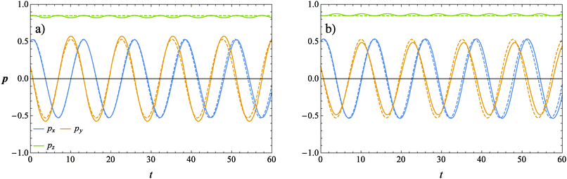 |
| | Fig. 3 Time evolution of the components of the orientation vector p for a puller (a) and a pusher (b) obtained from our perturbative solution. The solid lines represent the solution for De = 0.1 and B1* = 1. The dashed lines refer to the squirmer dynamics in a Newtonian suspending fluid (De = 0). | |
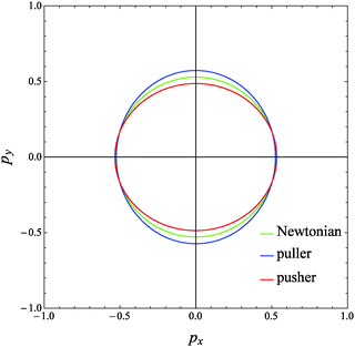 |
| | Fig. 4 Phase diagram of pyvs. px for a puller (blue line) and a pusher (red line) suspended in a viscoelastic fluid with De = 0.1 and B1* = 1 obtained from our perturbative solution. The same initial conditions as in Fig. 3a for the puller and in Fig. 3b for the pusher are used. The trend for a Newtonian suspending fluid (green curve) is also reported. | |
6 Numerical results
The orientational dynamics of an isolated microorganism suspended in a sheared unconfined viscoelastic fluid at non-vanishing Deborah numbers is investigated in this section. For all the three types of squirmers (neutral, puller and pusher), we perform numerical simulations by varying the Deborah number De in the range De ∈ [0.15, 2.0] and the dimensionless parameter B1* in the range B1* ∈ [0.2, 2]. The dimensionless constitutive parameters are kept constant as discussed in Section 3. For each set of parameters, we select different initial orientations in order to check the existence of multiple equilibrium orientations. Specifically, we choose eight different initial orientations in the semi-space z > 0 (for symmetry we can limit to one semi-space): p0 = (±0.8, 0, 0.6), p0 = (0, ±0.8, 0.6), p0 = (±0.4, 0, 0.9165) and p0 = (0, ±0.4, 0.9165). Thus, the particle is initially oriented at different distances from the vorticity axis, and along the negative and positive directions of the flow and gradient axes. The results for the neutral, puller and pusher squirmers with γ = 0 are reported in the next three subsections. In the last subsection, the effect of the third mode (γ ≠ 0) on the dynamics of the three kinds of microorganisms is shown.
6.1 Neutral squirmer
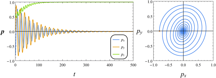
In Fig. 5, we report the time evolution of the components of the orientation vector p for a neutral squirmer with De = 1 and B1* = 1. The initial orientation is selected with p0 on the flow-vorticity plane near the flow direction. We observe damped oscillations towards the equilibrium solution (px, py, pz) = (0, 0, 1), corresponding to a drift of the microorganism orientation vector towards the vorticity axis. We repeated the simulations by varying the initial orientation as previously discussed, and always found the same long-time regime. Hence, we conclude that the vorticity axis is a stable equilibrium point regardless of the initial orientation p0. The orientation dynamics can be better visualized through a phase diagram showing the y-component of the orientation vector vs. its x-component (see the right panel of Fig. 5). The trend describes circular spiraling trajectories towards the origin of the diagram that represents the vorticity axis. We would like to remark that the just presented dynamics is different from that observed in a Newtonian suspending fluid where the orbits described by the orientation vector are periodic and no drift is found.
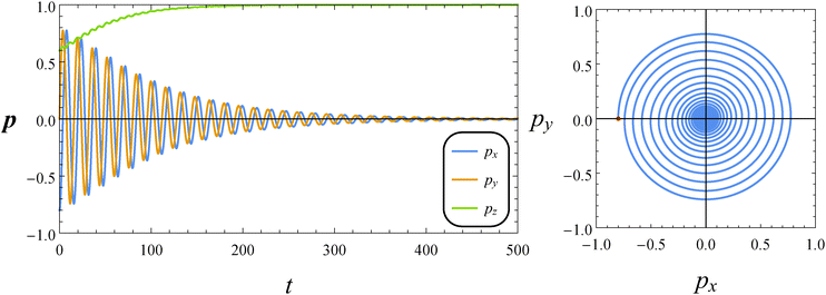 |
| | Fig. 5 Left: Time evolution of the components of the orientation vector p for a neutral squirmer (β = 0). The dimensionless parameters are De = 1 and B1* = 1. The initial orientation vector is p0 = (px, py, pz) = (−0.8, 0, 0.6). Right: Phase diagrams pyvs. px of the orbit depicted in the left panel. The red circle denotes the initial condition. | |
Further simulations have been carried out to investigate the influence of the parameters De and B1*. We found that, by decreasing these two parameters, the drift dynamics slows down. Indeed, as De is decreased, the system tends to the Newtonian case where no drift occurs. This is also confirmed by the perturbative analysis presented in the previous section where no drift is found at first-order in De. As B1* goes down, the case of a passive spherical particle in a viscoelastic fluid is recovered where, again, there is no drift (the only non-zero component of the angular velocity is that around the vorticity axis). Despite variations in De or B1* affecting the transients, the long-time regime remains the same, i.e., the vorticity axis, for any set of parameters in the investigated range.
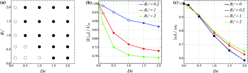
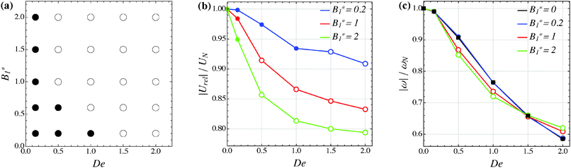
Our numerical results for a neutral squirmer are summarized in Fig. 6a, where a map of the equilibrium solutions is reported as a function of De and B1*. The black circle in this figure denotes vorticity alignment that, as just discussed, is found for any combination of De and B1* investigated in this work. It is worth emphasizing that, for De < 0.15, the drift towards or away from the vorticity axis is found to be negligible and, then, the corresponding data are not reported in Fig. 6a.
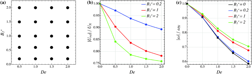 |
| | Fig. 6 (a) Map of the equilibrium solutions for the orientation vector of a neutral squirmer (β = 0). Filled symbols denote alignment along the vorticity axis. (b) Magnitude of the particle relative translational velocity as a function of the Deborah number for three different values of B1*. (c) Magnitude of the particle angular velocity as a function of the Deborah number for three different values of B1*. The passive particle case B1* = 0 is also reported (black symbols/line). The data in panels (b) and (c) are normalized by the translational and angular velocity of a squirmer in an unconfined sheared Newtonian fluid and refer to the long-time regime, i.e., once the particle has reached the equilibrium orientation. | |
In Fig. 6b and c, we show the trends of the particle kinematic quantities when the microorganism attains the equilibrium orientation as a function of the Deborah number and for three different values of the parameter B1*. Specifically, Fig. 6b reports the magnitude of the relative translational velocity of the microorganism |Urel| = |U − u∞| (i.e., the particle translational velocity without the background shear flow field). Fig. 6c shows the magnitude of the microorganism rotational velocity |ω|. Both velocities are normalized by the corresponding translational and rotational velocities of a squirmer in an unbounded sheared Newtonian fluid, denoted by UN = 2/3B1 and ωN = /2, respectively. Since a neutral squirmer always aligns along the vorticity direction, the magnitudes of the translational and angular velocities are |Uz| and |ωz|, respectively. The angular velocity of a passive spherical particle (B1* = 0) in a sheared viscoelastic fluid is also shown in Fig. 6c (black symbols and lines). In agreement with previous calculations for active particles in a quiescent viscoelastic fluid,22 fluid viscoelasticity slows down the squirmer translational velocity as compared to the Newtonian case. The trends also show a decreasing slope as De increases, again in agreement with the results of Zhu et al.,22 where the existence of a minimum in the normalized translational velocity as a function of the Weissenberg number (defined as Wi = λB1/(2R) = De B1*/2) was reported. Similar to a passive sphere, also the squirmer rotation rate slows down as fluid viscoelasticity increases. However, higher angular velocities are found for larger values of the parameter B1*, i.e., the squirmer rotates faster around the vorticity axis as the relative weight between the self-propulsion velocity and the flow characteristic velocity is higher.
6.2 Puller squirmer
Let us consider now the case of a puller with β = 1. As for the neutral squirmer, we carried out simulations for different combinations of De and B1*, and for several initial orientations. Similar to the neutral microorganism, no effect of the initial orientation is found. Hence, we only present results for a single initial orientation.
Fig. 7 reports the dynamics of the orientation vector of a puller swimmer with the same parameters (De = 1 and B1* = 1) and initial condition as in Fig. 5. As for the neutral squirmer, the orientation vector drifts towards the vorticity axis following a transient characterized by damped oscillations. The phase diagram shown in the right panel of Fig. 7, however, reveals that the spiraling orbit deforms from a circular to an elliptical shape, with the major axis crossing the first and third quadrants.
 |
| | Fig. 7 Left: Time evolution of the components of the orientation vector p for a puller (β = 1). The dimensionless parameters are De = 1 and B1* = 1. The initial orientation vector is p0 = (px, py, pz) = (−0.8, 0, 0.6). Right: Phase diagrams pyvs. px of the orbit depicted in the left panel. The red circle denotes the initial condition. | |
By changing the parameters De and B1*, however, a qualitatively different dynamics is found. For instance, for De = 1 and B1* = 0.2, both px and py oscillate with increasing amplitude as time goes on, up to spanning the whole range [−1, 1]. As a consequence, the trend of pz tends to zero at long times. Therefore, the equilibrium solution is a ‘tumbling’ of the orientation vector on the flow-gradient plane, around the vorticity axis. In conclusion, by decreasing the parameter B1*, the vorticity axis changes stability. We also found a much slower dynamics for B1* = 0.2 as compared to the case B1* = 1 (for B1* = 0.2, in 1000 dimensionless time units the equilibrium orientation is not reached whereas 500 time units are sufficient for the case depicted in Fig. 7).
The combined effect of De and B1* on the long-time regime is depicted in the solution map of Fig. 8a, where open symbols denote that the flow-gradient plane is a stable equilibrium solution. From the diagram we observe that, for De ≥ 1.5, the orientation vector of a puller always drifts towards the vorticity axis, whatever is the value of B1*. On the other hand, in the case of De = 0.15, for all the values of B1* investigated, the orientation vector of a puller moves towards the flow-gradient plane and the microorganism tumbles around the vorticity axis. Notice that this result is at variance with the perturbative solution derived in the previous section meaning that, already for De = 0.15, higher-order terms in De are required to predict the drift. For Deborah numbers ranging from 0.15 to 1.5, tumbling in the shear plane or alignment of the puller orientation vector along the vorticity axis occurs at low and high B1*-values, respectively.
 |
| | Fig. 8 (a) Map of the equilibrium solutions for the orientation vector of a puller (β = 1). Filled symbols denote alignment along the vorticity axis, whereas open circles denote tumbling around the vorticity axis. (b) Magnitude of the particle relative translational velocity as a function of the Deborah number for three different values of B1*. (c) Magnitude of the particle angular velocity as a function of the Deborah number for three different values of B1*. The passive particle case B1* = 0 is also reported (black symbols/line). The data in panels (b) and (c) are normalized by the translational and angular velocity of a squirmer in an unconfined sheared Newtonian fluid and refer to the long-time regime, i.e., once the particle has reached the equilibrium orientation. As in panel (a), closed and open circles refer to alignment along the vorticity axis and tumbling around the vorticity axis, respectively. In the latter case, the velocities are computed as an average over a period. | |
In Fig. 8b and c, the equilibrium translational and angular velocities of the puller squirmer are shown as a function of the Deborah number and for three different values of the parameter B1*. As for the neutral squirmer, the filled symbols represent the velocities attained when the squirmer aligns along the vorticity direction, corresponding to the closed circles in Fig. 8a. Now, however, for low values of De and B1*, the squirmer tumbles around the z-axis. In this case, the magnitude of the particle relative translational velocity in Fig. 8b is given by 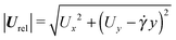 , whereas the magnitude of the angular velocity is again |ω| = |ωz|. Since both velocities are periodic, we take the average over a period. Similar to the neutral squirmer, both De and B1* slow down the translational and angular velocities as compared to the Newtonian case. A comparison between Fig. 6b and 8b also shows that a puller swims slower than a neutral squirmer, in agreement with previous numerical calculations.21
6.3 Pusher squirmer
In this subsection, we report the results of our numerical simulations for a pusher squirmer (β = −1). In the left panel of Fig. 9, the time evolution of the orientation vector components for De = 1 and B1* = 1 is shown. At variance with both the neutral and puller swimmers, for this set of parameters, the orientation vector drifts towards the shear plane which is a stable equilibrium solution. The spiraling orbit depicted in the right panel of Fig. 9 shows an elliptical shape with the major axis crossing the second and fourth quadrants (thus inverted as compared to that of a puller in the right panel of Fig. 7). By decreasing the value of B1*, the shear plane becomes unstable and the vorticity axis becomes an attractor. This is the case, for instance, by setting De = 1 and B1* = 0.2 (not shown).
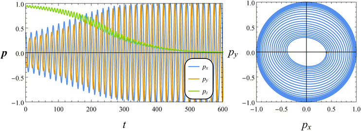 |
| | Fig. 9 Left: Time evolution of the components of the orientation vector p for a pusher (β = −1). The dimensionless parameters are De = 1 and B1* = 1. The initial orientation vector is p0 = (px, py, pz) = (0.4, 0, 0.9165). Right: Phase diagrams pyvs. px of the orbit depicted in the left panel. The red circle denotes the initial condition. | |
The overall picture of the long-time orientational dynamics of the pusher is depicted in the solution diagram of Fig. 10a. Here, the same notation as before is adopted. At large Deborah numbers (De ≥ 1.5), for all the values of B1* considered, the orientation vector drifts towards the shear plane and tumbles around the vorticity axis (open symbols in Fig. 10a); on the other hand, if De = 0.15, a pusher always aligns with the vorticity (closed symbols in Fig. 10a). As shown in Fig. 10a, in an intermediate range of the Deborah number (0.15 < De < 1.5), the stable equilibrium regime depends on B1*, with tumbling and vorticity alignment promoted at low and high values of this parameter.
 |
| | Fig. 10 (a) Map of the equilibrium solutions for the orientation vector of a pusher (β = −1). Filled symbols denote alignment along the vorticity axis, whereas open circles denote tumbling around the vorticity axis. (b) Magnitude of the particle relative translational velocity as a function of the Deborah number for three different values of B1*. (c) Magnitude of the particle angular velocity as a function of the Deborah number for three different values of B1*. The passive particle case B1* = 0 is also reported (black symbols/line). The data in panels (b) and (c) are normalized by the translational and angular velocity of a squirmer in an unconfined sheared Newtonian fluid and refer to the long-time regime, i.e., once the particle has reached the equilibrium orientation. As in panel (a), closed and open circles refer to alignment along the vorticity axis and tumbling around the vorticity axis, respectively. In the latter case, the velocities are computed as an average over a period. | |
Finally, the normalized equilibrium translational and angular velocities of the pusher squirmer are shown in Fig. 10b and c as a function of the Deborah number and for three different values of the parameter B1*. The same notation as in Fig. 8 is adopted. The translational velocity follows a trend similar to that observed for neutral and puller particles, decreasing with both De and B1*. However, for any value of these two parameters, the pusher swimming velocity is always faster than the corresponding velocity of neutral and puller squirmers. The angular velocity shows a different trend as compared to neutral and puller particles. Indeed, up to De = 1.5, higher B1*-values slow down the rotation rate. Only at De = 2, a faster rotation rate is found for increasing values of B1*. However, the maximum variation of the angular velocity from B1* = 0 to B1* = 2 is lower than 5–6%. Hence, the effect of B1* on the angular velocity for a pusher microorganism in a sheared viscoelastic fluid is relatively weak.
6.4 Effect of the third mode B3
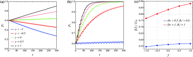
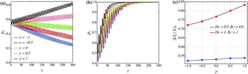
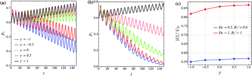
The effect of the third mode B3 through the dimensionless parameter γ on the particle dynamics is investigated in this section. Fig. 11–13 report the simulation results for the neutral, puller and pusher squirmers, respectively, with γ varied in the range [−1, 1]. Panels (a) and (b) show the particle orientational dynamics for (De, B1*) = (0.5, 0.6) and (De, B1*) = (1, 1), respectively. We selected these values since the corresponding points in the equilibrium solution maps of a puller (Fig. 8a) and a pusher (Fig. 10a) are close to the transition between vorticity alignment and tumbling on the flow-gradient plane, where a qualitative change in the rotational dynamics due to γ (if any) should be more evident. For the sake of clarity, only the z-component of the orientation vector is shown in these figures. For any investigated set of parameters, the only two equilibrium solutions are again vorticity alignment or tumbling on the flow-gradient plane. Furthermore, different initial orientations do not affect the long-time solution. Hence, the trends of pz are sufficient to determine the equilibrium orientation attained by the particle.
 |
| | Fig. 11 (a) and (b) z-component of the orientation vector of a neutral squirmer (β = 0) as a function of time for different values of the parameter γ. The data in panels (a) and (b) refer to (De, B1*) = (0.5, 0.6) and (De, B1*) = (1, 1), respectively. The colors in panel (b) correspond to the same γ-values as reported in panel (a). (c) Magnitude of the particle translational velocity as a function of the parameter γ for the two sets of (De, B1*) as in panels (a) and (b). The translational velocities are computed in the moving reference frame and are normalized by the translational velocity of a squirmer in an unconfined sheared Newtonian fluid and refer to the long-time regime, i.e., once the particle has reached the equilibrium orientation. | |
 |
| | Fig. 12 (a) and (b) z-component of the orientation vector of a puller (β = 1) as a function of time for different values of the parameter γ. The data in panels (a) and (b) refer to (De, B1*) = (0.5, 0.6) and (De, B1*) = (1, 1), respectively. The colors in panel (b) correspond to the same γ-values as reported in panel (a). (c) Magnitude of the particle translational velocity as a function of the parameter γ for the two sets of (De, B1*) as in panels (a) and (b). The translational velocities are computed in the moving reference frame and are normalized by the translational velocity of a squirmer in an unconfined sheared Newtonian fluid and refer to the long-time regime, i.e., once the particle has reached the equilibrium orientation. | |
 |
| | Fig. 13 (a) and (b) z-component of the orientation vector of a pusher (β = −1) as a function of time for different values of the parameter γ. The data in panels (a) and (b) refer to (De, B1*) = (0.5, 0.6) and (De, B1*) = (1, 1), respectively. The colors in panel (b) correspond to the same γ-values as reported in panel (a). (c) Magnitude of the particle translational velocity as a function of the parameter γ for the two sets of (De, B1*) as in panels (a) and (b). The translational velocities are computed in the moving reference frame and are normalized by the translational velocity of a squirmer in an unconfined sheared Newtonian fluid and refer to the long-time regime, i.e., once the particle has reached the equilibrium orientation. | |
The data reported in these figures show that negative (positive) values of γ tend to slow down (speed up) the drift of the orientation vector towards the vorticity axis or speed up (slow down) the drift of p towards the flow-gradient plane. This is clearly visible for the neutral and puller squirmers with (De, B1*) = (1, 1) (Fig. 11b and 12b) where vorticity alignment is reached in times that significantly depend on γ. A similar effect of γ is also found for a pusher (Fig. 13b) where the tumbling on the flow-gradient plane is reached at a higher or lower rate whether γ is negative or positive, respectively. Notably, for the highest γ-value investigated (black line), the equilibrium dynamics changes from tumbling to vorticity alignment.
The influence of the third mode on the equilibrium orientation is more relevant for the case (De, B1*) = (0.5, 0.6) reported in panels (a) of the previous figures: the equilibrium orientation for the neutral and pusher squirmers switches from vorticity alignment to tumbling by decreasing γ from 0 to −0.5; the opposite is observed for a puller by increasing γ from 0 to 0.5. Furthermore, as before, higher and lower γ-values speed up vorticity alignment and tumbling, respectively. In conclusion, the third mode of Blake's expansion can change the equilibrium orientation attained by the particle, especially for low values of the parameters De and B1*. It is important to point out, however, that the effect of the parameter γ is decoupled from β in the sense that, regardless of the kind of microorganism, positive or negative γ-values promote vorticity alignment or tumbling on the flow-gradient plane.
Panels (c) of the previous figures show the normalized translational velocity of the microorganism for different values of the parameters γ and for the two sets of (De, B1*) corresponding to the data in panels (a) and (b). For all the three kinds of squirmer, an increasing translational velocity is found as γ increases. This effect is more evident for higher values of De and B1*, and for a neutral and a puller squirmer. Finally, we mention that the equilibrium particle angular velocity is essentially unaffected by the third mode, with the maximum deviations in the investigated range of γ being lower than 1%.
6.5 Discussion
The numerical simulation results presented in the previous sections clearly show a dramatic effect of fluid viscoelasticity on the squirmer dynamics as compared to the Newtonian case. Previous works on passive particles in sheared viscoelastic liquids have shown that the first normal stress difference is the main cause of the different particle dynamics as compared to Newtonian suspensions. This is the case, for instance, of the slowing down effect of spherical particles46 and the existence of preferential orientations of non-spherical particles.48 Since both phenomena have been found for a microorganism suspended in a viscoelastic fluid under shear, it is likely that the first normal stresses are the main source of the peculiar dynamics reported in the present work as well. In particular, the drift of the orientational vector of pusher microorganisms towards the vorticity axis or the flow-gradient plane at low and high Deborah numbers is similar to the orientational dynamics of a prolate ellipsoidal passive particle in a sheared viscoelastic liquid.48,55 However, it has to be pointed out that some relevant features observed for passive spheroids are not found for spherical active particles: (i) a spheroid with the major axis on the xy-plane reaches an equilibrium orientation near the flow axis if the aspect ratio is sufficiently large whereas a spherical squirmer tumbles around the z-axis; (ii) for intermediate De, the major axis of a spheroid reaches an equilibrium orientation between the vorticity and the flow axis; (iii) the latter solution can coexist with vorticity alignment. The more complex scenario reported for spheroidal particles might be attributed to their anisotropic shape and could be observed for non-spherical active particles.
The rheological properties of the suspending fluid might also have an important role in the microorganism dynamics. We have already mentioned that the first normal stresses are the main factors responsible for the observed drift. It is worthwhile to point out, however, that the Giesekus model employed in this work also predicts shear-thinning and a non-zero second normal stress difference in shear flow. Both these features might contribute in some way to the observed particle dynamics (as happens, for instance, for spheroidal passive particles48). To clarify the detailed effect of the fluid rheology, the constitutive parameters of the viscoelastic model should be varied and simulations by changing the constitutive model are needed. This investigation will be part of future work.
A comparison between the solution maps for a puller reported in Fig. 8a and a pusher reported in Fig. 10a shows that, for a fixed couple (De, B1*) (and for γ = 0), the two kinds of microorganisms have an ‘opposite’ behavior, i.e., if the pusher orientation vector drifts towards the shear plane, a puller aligns with the vorticity and vice versa. This opposite behavior is not completely unexpected because their flow fields in a Newtonian fluid are also inverse. As previously mentioned, the normal stresses are expected to be responsible for the orientation vector drift. The inverse flow field around pushers and pullers leads to an inverse shear rate gradient profile as well that, in turn, generates an opposite distribution of normal stresses around the surface, possibly justifying the observed behavior. This interesting feature might be exploited to obtain a separation of swimming microorganisms based on their propulsion mechanism.
Finally, it is interesting to compare the relevant time scales involved in real microorganism dynamics. Several characteristic times can be identified: (i) the time tb for the boundary actuation that is related to the frequency of the cilia beating on the organism surface; (ii) the characteristic time required for the viscoelastic stress development tv that is related to the fluid relaxation time λ; (iii) the flow characteristic time tf related to 1/; (iv) the characteristic time tm of the microorganism swimming that is related to R/B1 (i.e. the time required to swim a distance equal to its radius); (v) the time tT needed for a revolution of the orientation vector around the vorticity axis, i.e., the characteristic time of the oscillations in Fig. 5, 7 and 9, that is related to the rotation period T = 2π/ω; and (vi) the time ts required to achieve the equilibrium orientation. The fluid, flow and swimming time scales can be combined as discussed in Section 3 to give De and B1*. The values selected for these two parameters give (tv) ≈ (tf) ≈ (tm). Typical values of tm of real microorganisms fall in the range [0.1–1 s].40,41 Thus, the interval of B1* investigated in the present paper corresponds to shear rates that are easily accessible through conventional rheometers.56 Hence, by employing dilute and semi-dilute polymer suspensions, it should be possible to experimentally observe some of the effects described in the present paper. The rotation period T depends on ω, which, in turn, depends on De, B1* and β. However, in the range of parameters investigated in this work, the microorganism angular velocity is of the same order of magnitude as in the Newtonian case ωN = /2 (see, e.g., Fig. 6c, 8c and 10c). Thus, tT is slightly less than one order of magnitude higher than tf. The time ts needed to reach the equilibrium orientation depends on all the relevant dimensionless numbers as well as on the initial orientation. However, it is always found that ts is much larger than tT as clearly visible in Fig. 5, 7 and 9 where several oscillations are required before reaching the steady-state condition. Finally, the characteristic time of the microorganism’s beating cilia tb is typically 10–20 milliseconds.57 Hence, in the range of parameters investigated in this work, such a time is significantly lower than the other aforementioned characteristic times justifying the use of a steady-state boundary condition on the particle surface.
7 Conclusions
In this paper, we investigated the orientational dynamics of a swimming microorganism suspended in a sheared unconfined viscoelastic fluid. In the limit of small Deborah numbers, we performed an asymptotic expansion accurate to first-order in the Deborah number yielding an analytical expression for the rotational velocity of the microorganism. The perturbative analysis revealed that, at low Deborah numbers, swimming microorganisms do not attain any preferential orientation nor migrate towards a stable orbit, and the dynamics remains qualitatively similar to the Newtonian case.
The analysis was extended to high Deborah numbers by means of direct finite element simulations. The numerical results show that, at variance with the Newtonian case, spherical microorganisms in a viscoelastic fluid attain a preferential orientation that depends on the Deborah number De, the relative weight between the self-propulsion velocity and the flow characteristic velocity B1*, and the type of swimming (β, γ). Specifically, for γ = 0, neutral microorganisms always align with the vorticity axis. On the other hand, tumbling around the vorticity axis is found for pullers and pushers at low and high De-values, respectively. For intermediate De-values, the stable long-time solution depends on the value of B1*. We emphasize that, for a fixed set of De and B1*, puller and pusher squirmers always show an opposite behavior, suggesting a possible technique to separate microorganisms based on their propulsion mechanism. Non-zero values of γ can modify the equilibrium orientation as compared to the case γ = 0 in a direction that does not depend on the kind of squirmer. For some combinations of parameters, pushers and pullers can also tend towards the same long-time regime.
The results presented in this work can be extended in several ways. The effect of the fluid rheological properties as well as of a more realistic time dependent boundary condition for the beating cilia of the microorganism on the particle dynamics can be investigated. Finally, the orientational dynamics found in this study also suggests that the rheology of dilute microorganism suspensions in viscoelastic fluids could be very different from the Newtonian counterpart. The predictions of the rheology behavior of active viscoelastic suspensions will be part of future work.
Appendix A: zeroth-order problem
By substituting eqn (23) into eqn (15) and (16), and retaining only the zeroth-order terms (i.e., the terms that do not depend on De), we obtain the following dimensionless equations:with u0 the zeroth-order flow field and Σ0 the zeroth-order stress tensor given by| | | Σ0 = − p0I + (1 − ηr)(∇u0 + ∇uT0) + τ0 | (29) |
From eqn (5), the zeroth-order viscoelastic stress iswhich can be substituted in eqn (29) to give| | | Σ0 = −p0I + (∇u0 + ∇uT0) | (31) |
The boundary condition on the particle surface, in a reference frame translating with the particle, is| | 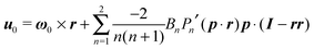 | (32) |
with r a point on the squirmer surface, and far from the organism:The force- and torque-free conditions to the zeroth-order are given by| |  | (34) |
| |  | (35) |
Notice that, in the low Deborah number analysis, the viscoelastic stress tensor instantaneously reaches its pseudo-steady value, and hence no initial condition is required for it.
Due to the linearity of the Stokes equations, the solution of the above system of partial differential equations is the superposition of the solution for the motion of a squirmer in a quiescent Newtonian fluid with arbitrary orientation p and that of a ‘passive’ sphere suspended in a Newtonian fluid undergoing a shear flow u∞ at infinity. Hence, the total zeroth-order translational velocity is given by the velocity of an unconfined squirmer in a quiescent Newtonian fluid  31 (as a ‘passive’ sphere in shear flow has no translational velocity in the reference frame we have chosen, see Section 3). The total rotational velocity is given by the rotational velocity of a ‘passive’ sphere in a Newtonian shear flow
  with k the z-axis unit vector (as the microorganism has no self-induced rotational velocity). The zeroth-order translational and rotational velocities reported above can also be derived from the reciprocal theorem as previously shown in the literature8 and summarized in a recent book.58 The total Newtonian velocity flow field u0 can be written as the sum of an ‘active’ contribution u0,a and a ‘passive’ contribution u0,p. The ‘active’ flow field is given by31
| | 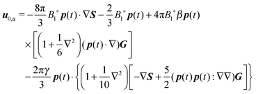 | (36) |
where
S is the Green's function for a point source in an unconfined Newtonian fluid:
49| |  | (37) |
with
x the position vector of a point in the space and
r its magnitude. The tensor
G is instead the Green's function for a point force in an unconfined fluid:
49| | 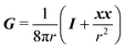 | (38) |
The ‘passive’ contribution is well-known in the literature, as it was originally derived by Einstein, and is reported here employing the nomenclature used in Greco
et al.:
59| | 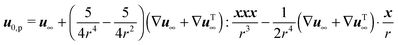 | (39) |
Finally, the zeroth-order (Newtonian) flow field is obtained as
Appendix B: first-order problem
The dimensionless equations of the first-order problem are found by substituting eqn (23) into eqn (15) and (16) and retaining only the first-order terms (i.e., the terms that depend linearly on De):with u1 the first-order flow field and Σ1 the first-order stress tensor given by| | | Σ1 = −p1I + (1 − ηr)(∇u1 + ∇uT1) + τ1 | (43) |
where τ1 is| | 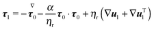 | (44) |
Substituting the expression of τ1 into eqn (43) we obtain| | 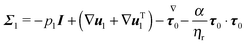 | (45) |
Since only the first two terms of the right-hand side of eqn (45) are the unknowns, it is convenient to introduce the following definition:| | | σ1 = −p1I + (∇u1 + ∇uT1) | (46) |
Eqn (42) is then rewritten as| |  | (47) |
where the left-hand side contains the unknowns and the right-hand side contains (known) contributions from the zeroth-order solution. We emphasize that the time derivative of the zeroth-order flow field appearing in  is computed by time differentiation and, thus, no specific treatment is required.
The first-order mass balance in eqn (41) and the first-order momentum balance in eqn (42) are equipped with the first-order boundary conditions on the particle surface, in a reference frame translating with the particle:
and far from the organism:
Finally, the force- and torque-free conditions hold for the first-order problem:
| |  | (50) |
| |  | (51) |
B.1 First-order rotational velocity
In principle, the unknown fields p1 and u1 plus the first-order squirmer translational U1 and rotational ω1 velocities can be obtained from the solution of eqn (41), (47), (50) and (51). In what follows, however, we show that the first-order squirmer rotational velocity ω1 can be obtained without the explicit knowledge of the first-order velocity and pressure fields, by making use of the generalized reciprocity theorem49 from Stokes flow theory.
We proceed by defining an auxiliary Stokes problem, namely, the rotation of a sphere with a rotational velocity ![[small omega, Greek, circumflex]](https://www.rsc.org/images/entities/b_i_char_e0b4.gif) , suspended in an unbounded quiescent Newtonian fluid. (All the quantities related to the auxiliary problem are denoted with a hat superscript.) We emphasize that in principle any Stokes problem might be chosen as an auxiliary problem in the reciprocity theorem. Typical choices are rigid body motions like translation and rotation.20 The choice of the auxiliary problem made in the present work is motivated by the fact that we are interested in the rotational rate of the particle and not in the translational velocity. The dimensionless equations governing this problem are
, suspended in an unbounded quiescent Newtonian fluid. (All the quantities related to the auxiliary problem are denoted with a hat superscript.) We emphasize that in principle any Stokes problem might be chosen as an auxiliary problem in the reciprocity theorem. Typical choices are rigid body motions like translation and rotation.20 The choice of the auxiliary problem made in the present work is motivated by the fact that we are interested in the rotational rate of the particle and not in the translational velocity. The dimensionless equations governing this problem are
| | ∇·![[capital Sigma, Greek, circumflex]](https://www.rsc.org/images/entities/b_i_char_e139.gif) = 0 = 0 | (53) |
The stress tensor of the auxiliary problem is given by
| | = −![[p with combining circumflex]](https://www.rsc.org/images/entities/i_char_0070_0302.gif) I + ∇û + ∇ûT I + ∇û + ∇ûT | (54) |
The boundary conditions to the auxiliary Stokes problem are
| | | û = × r | (55) |
on the spherical surface and
far from the sphere.
The derivation in this appendix closely follows that originally reported by Lauga,20,60 subsequently used in Datt et al.38 and De Corato et al.,19 and recently summarized in a book chapter.18 The generalized reciprocity theorem states that
| |  | (57) |
We can make some simplifications in the above equation: (i) the second volume integral of the right-hand side is identically zero (see
eqn (53)); (ii) the velocities
û and
u1 are replaced by the expressions given in
eqn (55) and (48), respectively, and the well known property of cross product (
a ×
b)·
c =
a·(
b ×
c) is used; (iii) in the first volume integral of the right-hand side, ∇·
σ1 is substituted by the expression given in
eqn (47). Hence,
eqn (57) becomes
| |  | (58) |
By using the identity
w·∇·
W = ∇·(
w·
W) − ∇
w:
W (
w and
W are a vector and a tensor, respectively), we rewrite the volume integral in
eqn (58) as the sum of two volume integrals, and transform the volume integral containing the overall divergence into a surface integral to obtain
| |  | (59) |
Eqn (59) can be further manipulated: (i) in the third surface integral the velocity on the boundary is substituted with the boundary condition in
eqn (55) and the aforementioned property of cross product is used; notice that, after this substitution, the rotational velocity
appears in the third integral; (ii) such rotational velocity
is constant and is put outside the integrals; (iii) also the rotational velocity
ω1 in the second surface integral is constant and is put outside the integral; (iv) the resulting integral expresses the drag torque on the rotating sphere in the auxiliary problem and it is simply −8π
. Therefore, we get
| | 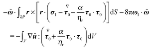 | (60) |
The surface integral in the above equation is identically zero as it expresses the first-order torque-free condition
(51). Thus, we have
| | 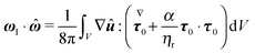 | (61) |
The
x,
y and
z components of the first-order rotational velocity
ω1 can therefore be computed by evaluating the integral on the right-hand side (which has an analytical solution) employing three different auxiliary problems, namely the rotation of a sphere around the
x,
y and
z axis, respectively. In conclusion, we end up with the following expression for the first-order angular velocity:
| |  | (62) |
with
i,
j, and
k the
x-,
y-, and
z-axis unit vectors, respectively.
References
- K. M. Ottemann and J. F. Miller, Roles for motility in bacterial-host interactions, Mol. Microbiol., 1997, 24(6), 1109–1117 CAS.
- N. A. Hill and T. J. Pedley, Bioconvection, Fluid Dynam. Res., 2005, 37(1), 1–20 CrossRef.
- N. Darnton, L. Turner, K. Breuer and H. C. Berg, Moving fluid with bacterial carpets, Biophys. J., 2004, 86(3), 1863–1870 CrossRef CAS PubMed.
- D. L. Koch and G. Subramanian, Collective hydrodynamics of swimming microorganisms: living fluids, Annu. Rev. Fluid Mech., 2011, 43, 637–659 CrossRef.
- E. Lauga, Bacterial hydrodynamics, Annu. Rev. Fluid Mech., 2016, 48, 105–130 CrossRef.
- J. Elgeti, R. G. Winkler and G. Gompper, Physics of microswimmers-single particle motion and collective behavior: a review, Rep. Prog. Phys., 2015, 78(5), 056601 CrossRef CAS PubMed.
-
S. Childress, Mechanics of Swimming and Flying, Cambridge Univ Press, 1981 Search PubMed.
- H. A. Stone and A. D. T. Samuel, Propulsion of microorganisms by surface distortions, Phys. Rev. Lett., 1996, 77(19), 4102 CrossRef CAS PubMed.
- C. Dombrowski, L. Cisneros, S. Chatkaew, R. E. Goldstein and J. O. Kessler, Shearing active gels close to the isotropic-nematic transition, Phys. Rev. Lett., 2004, 93(9), 098103 CrossRef PubMed.
- I. H. Riedel, K. Kruse and J. Howard, A self-organized vortex array of hydrodynamically entrained sperm cells, Science, 2005, 308(5732), 300–303 CrossRef PubMed.
- E. Lauga and T. R. Powers, The hydrodynamics of swimming microorganisms, Rep. Prog. Phys., 2009, 72(9), 096601 CrossRef.
- K. Miki and D. E. Clapham, Rheotaxis guides mammalian sperm, Curr. Biol., 2013, 23(6), 443–452 CrossRef CAS PubMed.
- V. Kantsler, J. Dunkel, M. Blayney and R. E. Goldstein, Rheotaxis facilitates upstream navigation of mammalian sperm cells, eLife, 2014, 3, e02403 Search PubMed.
- K. Ishimoto and E. A. Gaffney, Fluid flow and sperm guidance: a simulation study of hydrodynamic sperm rheotaxis, J. R. Soc., Interface, 2015, 12(106), 20150172 CrossRef PubMed.
- D. Saintillan, The dilute rheology of swimming suspensions: a simple kinetic model, Exp. Mech., 2010, 50(9), 1275–1281 CrossRef.
- H. M. López, J. Gachelin, C. Douarche, H. Auradou and E. Clément, Turning bacteria suspensions into superfluids, Phys. Rev. Lett., 2015, 115(2), 028301 CrossRef PubMed.
- C. Montecucco and R. Rappuoli, Living dangerously: how Helicobacter pylori survives in the human stomach, Nat. Rev. Mol. Cell Biol., 2001, 2(6), 457–466 CrossRef CAS PubMed.
-
G. J. Elfring and E. Lauga, Theory of locomotion through complex fluids, in Complex Fluids in Biological Systems, ed. S. E. Spagnolie, Springer, 2015, pp. 283–317 Search PubMed.
- M. De Corato, F. Greco and P. L. Maffettone, Locomotion of a microorganism in weakly viscoelastic liquids, Phys. Rev. E: Stat., Nonlinear, Soft Matter Phys., 2015, 92(5), 053008 CrossRef CAS PubMed.
- E. Lauga, Locomotion in complex fluids: integral theorems, Phys. Fluids, 2014, 26(8), 081902 CrossRef.
- L. Zhu, E. Lauga and L. Brandt, Self-propulsion in viscoelastic fluids: pushers vs. pullers, Phys. Fluids, 2012, 24(5), 051902 CrossRef.
- L. Zhu, M. Do-Quang, E. Lauga and L. Brandt, Locomotion by tangential deformation in a polymeric fluid, Phys. Rev. E: Stat., Nonlinear, Soft Matter Phys., 2011, 83(1), 011901 CrossRef PubMed.
- E. Lauga, Propulsion in a viscoelastic fluid, Phys. Fluids, 2007, 19(8), 083104 CrossRef.
- S. Yazdi, A. M. Ardekani and A. Borhan, Locomotion of microorganisms near a no-slip boundary in a viscoelastic fluid, Phys. Rev. E: Stat., Nonlinear,
Soft Matter Phys., 2014, 90(4), 043002 CrossRef PubMed.
- G.-J. Li, A. Karimi and A. M. Ardekani, Effect of solid boundaries on swimming dynamics of microorganisms in a viscoelastic fluid, Rheol. Acta, 2014, 53(12), 911–926 CrossRef CAS PubMed.
- S. Yazdi, A. M. Ardekani and A. Borhan, Swimming dynamics near a wall in a weakly elastic fluid, J. Nonlinear Sci., 2015, 25(5), 1153–1167 CrossRef CAS.
- A. M. Ardekani and E. Gore, Emergence of a limit cycle for swimming microorganisms in a vortical flow of a viscoelastic fluid, Phys. Rev. E: Stat., Nonlinear, Soft Matter Phys., 2012, 85(5), 056309 CrossRef CAS PubMed.
- A. J. T. M. Mathijssen, T. N. Shendruk, J. M. Yeomans and A. Doostmohammadi, Upstream swimming in microbiological flows, Phys. Rev. Lett., 2016, 116(2), 028104 CrossRef PubMed.
- G. D'Avino and P. L. Maffettone, Particle dynamics in viscoelastic fluids, J. Non-Newtonian Fluid Mech., 2015, 215, 80–104 CrossRef.
- M. J. Lighthill, On the squirming motion of nearly spherical deformable bodies through liquids at very small Reynolds numbers, Comm. Pure Appl. Math., 1952, 5(2), 109–118 CrossRef.
- J. R. Blake, A spherical envelope approach to ciliary propulsion, J. Fluid Mech., 1971, 46(1), 199–208 CrossRef.
- T. Ishikawa and T. J. Pedley, The rheology of a semi-dilute suspension of swimming model micro-organisms, J. Fluid Mech., 2007, 588, 399–435 Search PubMed.
- A. A. Evans, T. Ishikawa, T. Yamaguchi and E. Lauga, Orientational order in concentrated suspensions of spherical microswimmers, Phys. Fluids, 2011, 23(11), 111702 CrossRef.
- K. Ishimoto and E. A. Gaffney, Squirmer dynamics near a boundary, Phys. Rev. E: Stat., Nonlinear, Soft Matter Phys., 2013, 88(6), 062702 CrossRef PubMed.
- G. J. Li and A. M. Ardekani, Hydrodynamic interaction of microswimmers near a wall, Phys. Rev. E: Stat., Nonlinear, Soft Matter Phys., 2014, 90(1), 013010 CrossRef PubMed.
- B. Delmotte, E. E. Keaveny, F. Plouraboué and E. Climent, Large-scale simulation of steady and time-dependent active suspensions with the force-coupling method, J. Comput. Phys., 2015, 302, 524–547 CrossRef.
- T. Ishikawa, M. P. Simmonds and T. J. Pedley, Hydrodynamic interaction of two swimming model micro-organisms, J. Fluid Mech., 2006, 568, 119–160 CrossRef.
- C. Datt, L. I. Zhu, G. J. Elfring and O. S. Pak, Squirming through shear-thinning fluids, J. Fluid Mech., 2015, 784, R1 CrossRef.
-
R. G. Larson, Constitutive Equations for Polymer Melts and Solutions: Butterworths Series in Chemical Engineering, Butterworth-Heinemann, 2013 Search PubMed.
- K. Drescher, R. E. Goldstein, N. Michel, M. Polin and I. Tuval, Direct measurement of the flow field around swimming microorganisms, Phys. Rev. Lett., 2010, 105(16), 168101 CrossRef PubMed.
- T. Ishikawa and M. Hota, Interaction of two swimming Paramecia, J. Exp. Biol., 2006, 209(22), 4452–4463 CrossRef PubMed.
- C. Geuzaine and J.-F. Remacle, Gmsh: a 3d finite element mesh generator with built-in pre- and post-processing facilities, Int. J. Numer. Meth. Eng., 2009, 79(11), 1–24 Search PubMed.
- A. N. Brooks and T. J. R. Hughes, Streamline Upwind/Petrov-Galerkin formulations for convection dominated flows with particular emphasis on the incompressible Navier-Stokes equations, Comp. Meth. Appl. Mech. Eng., 1982, 32, 199–259 CrossRef.
- R. Fattal and R. Kupferman, Constitutive laws for the matrix-logarithm of the conformation tensor, J. Non-Newtonian Fluid Mech., 2004, 123, 281–285 CrossRef CAS.
- M. A. Hulsen, R. Fattal and R. Kupferman, Flow of viscoelastic fluids past a cylinder at high Weissenberg number: stabilized simulations using matrix logarithms, J. Non-Newtonian Fluid Mech., 2005, 127, 27–39 CrossRef CAS.
- G. D'Avino, M. A. Hulsen, F. Snijkers, J. Vermant, F. Greco and P. L. Maffettone, Rotation of a sphere
in a viscoelastic liquid subjected to shear flow. Part I: simulation results, J. Rheol., 2008, 52(6), 1331–1346 CrossRef.
-
D. C. Rapaport, The Art of Molecular Dynamics Simulation, Cambridge University Press, New York, 1995 Search PubMed.
- G. D'Avino, M. A. Hulsen, F. Greco and P. L. Maffettone, Bistability and metabistability scenario in the dynamics of an ellipsoidal particle in a sheared viscoelastic fluid, Phys. Rev. E: Stat., Nonlinear, Soft Matter Phys., 2014, 89(4), 043006 CrossRef PubMed.
-
C. Pozrikidis, Boundary Integral and Singularity Methods for Linearized Viscous Flow, Cambridge University Press, 1992 Search PubMed.
- S. E. Spagnolie and E. Lauga, Hydrodynamics of self-propulsion near a boundary: predictions and accuracy of far-field approximations, J. Fluid Mech., 2012, 700, 105–147 CrossRef.
-
E. Guazzelli and J. F. Morris, A Physical Introduction to Suspension Dynamics, Cambridge University Press, 2012 Search PubMed.
- P. Brunn, The slow motion of a sphere in a second-order fluid, Rheol. Acta, 1976, 15(3), 163–171 CrossRef CAS.
- F. Gauthier, H. L. Goldsmith and S. G. Mason, Particle motions in non-newtonian media, Rheol. Acta, 1971, 10(3), 344–364 CrossRef CAS.
-
A. Morozov and S. E. Spagnolie, Introduction to complex fluids, in Complex Fluids in Biological Systems, Springer, 2015, pp. 3–52 Search PubMed.
- D. Z. Gunes, R. Scirocco, J. Mewis and J. Vermant, Flow-induced orientation of non-spherical particles: effect of aspect ratio and medium rheology, J. Non-Newtonian Fluid Mech., 2008, 155(1), 39–50 CrossRef CAS.
-
C. W. Macosko, Rheology: Principles, Measurements and Applications, Wiley Online Library, 1994 Search PubMed.
- C. Brennen, An oscillating-boundary-layer theory for ciliary propulsion, J. Fluid Mech., 1974, 65(4), 799–824 CrossRef.
-
S. Spagnolie, Complex Fluids in Biological Systems: Experiment, Theory and Computation, Springer, 2014 Search PubMed.
- F. Greco, G. D'Avino and P. L. Maffettone, Rheology of a dilute suspension of rigid spheres in a second order fluid, J. Non-Newtonian Fluid Mech., 2007, 147(1), 1–10 CrossRef CAS.
- E. Lauga, Life at high Deborah number, Europhys. Lett., 2009, 86(6), 64001 CrossRef.
|
| This journal is © The Royal Society of Chemistry 2017 |
Click here to see how this site uses Cookies. View our privacy policy here. 
 is called puller, as its maximum tangential velocity is on the frontal hemisphere; in other words, a puller generates propulsion from the front. Squirmers with a negative ratio
  are called pushers, as they generate propulsion from the rear. When B2 = 0, the organism is called neutral. The B3 mode is responsible for a force quadrupole in the fluid and can be used to model fore–aft symmetric differences in cilia beating. In a quiescent Newtonian fluid, the translational velocity of the squirmer is simply equal to
  as shown in the original paper of Blake.31 Note that a squirmer has no self-induced rotational velocity as the slip velocity in eqn (1) through which the microorganism propels is axisymmetric.


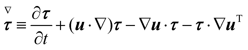


 which represents the ratio between the microorganism and flow characteristic velocities;
  which denotes the type of squirmer (neutral, puller or pusher); and
  which is the ratio between the third and the first mode of Blake's expansion. A Newtonian fluid with constant viscosity η0 is obtained by setting De = 0, whereas a ‘passive’ sphere undergoing shear flow in a viscoelastic fluid is obtained for B1* = 0. Realistic values of β range between −1 and 1.40,41 In this paper, we consider the three kinds of microorganisms by setting β = 0 for the neutral, β = 1 for the puller and β = −1 for the pusher. Experimental results on ciliated organisms have shown that the third mode is generally lower than the first one.41 In this work, we selected values of γ in the range [−1, 1]. Further rheological dimensionless parameters are the mobility parameter α and the viscosity ratio ηr = ηp/η0; unless otherwise specified, we set α = 0.2 (denoting a shear-thinning fluid) and ηr = 0.91. Finally, the last dimensionless parameter to be specified is the initial orientation p0.


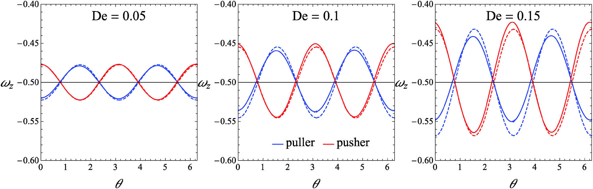


 , whereas the magnitude of the angular velocity is again |ω| = |ωz|. Since both velocities are periodic, we take the average over a period. Similar to the neutral squirmer, both De and B1* slow down the translational and angular velocities as compared to the Newtonian case. A comparison between Fig. 6b and 8b also shows that a puller swims slower than a neutral squirmer, in agreement with previous numerical calculations.21


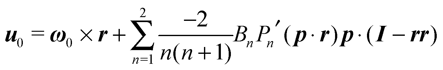

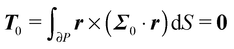
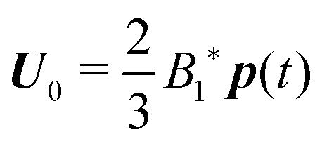 31 (as a ‘passive’ sphere in shear flow has no translational velocity in the reference frame we have chosen, see Section 3). The total rotational velocity is given by the rotational velocity of a ‘passive’ sphere in a Newtonian shear flow
  with k the z-axis unit vector (as the microorganism has no self-induced rotational velocity). The zeroth-order translational and rotational velocities reported above can also be derived from the reciprocal theorem as previously shown in the literature8 and summarized in a recent book.58 The total Newtonian velocity flow field u0 can be written as the sum of an ‘active’ contribution u0,a and a ‘passive’ contribution u0,p. The ‘active’ flow field is given by31

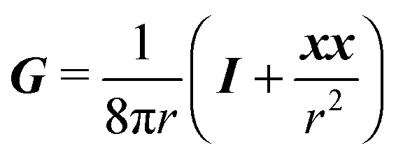
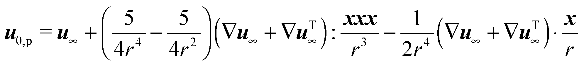

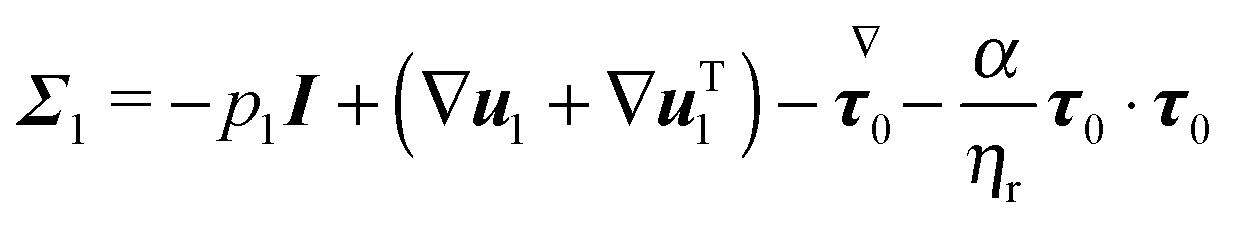

 is computed by time differentiation and, thus, no specific treatment is required.