
 Open Access Article
 This Open Access Article is licensed under a Creative Commons Attribution-Non Commercial 3.0 Unported Licence
Introducing DDEC6 atomic population analysis: part 3. Comprehensive method to compute bond orders†
Thomas A. Manz
Department of Chemical & Materials Engineering, New Mexico State University, Las Cruces, NM 88003-8001, USA. E-mail: tmanz@nmsu.edu
First published on 25th September 2017
Abstract
Developing a comprehensive method to compute bond orders is a problem that has eluded chemists since Lewis's pioneering work on chemical bonding a century ago. Here, a computationally efficient method solving this problem is introduced and demonstrated for diverse materials including elements from each chemical group and period. The method is applied to non-magnetic, collinear magnetic, and non-collinear magnetic materials with localized or delocalized bonding electrons. Examples studied include the stretched O2 molecule, 26 diatomic molecules, 3d and 5d transition metal solids, periodic materials with 1 to 8748 atoms per unit cell, a biomolecule, a hypercoordinate molecule, an electron deficient molecule, hydrogen bound systems, transition states, Lewis acid–base complexes, aromatic compounds, magnetic systems, ionic materials, dispersion bound systems, nanostructures, and other materials. From near-zero to high-order bonds were studied. Both the bond orders and the sum of bond orders for each atom are accurate across various bonding types: metallic, covalent, polar-covalent, ionic, aromatic, dative, hypercoordinate, electron deficient multi-centered, agostic, and hydrogen bonding. The method yields similar results for correlated wavefunction and density functional theory inputs and for different SZ values of a spin multiplet. The method requires only the electron and spin magnetization density distributions as input and has a computational cost scaling linearly with increasing number of atoms in the unit cell. No prior approach is as general. The method does not apply to electrides, highly time-dependent states, some extremely high-energy excited states, and nuclear reactions.
1. Introduction
Bond order helps us understand and predict chemical behaviors. In organic chemistry, electrophilic and nucleophilic addition reactions can take place across a multiple-order bond but not across a single-order bond.1 Thus, if we want to determine whether a bond can potentially undergo an electrophilic or nucleophilic addition reaction, we first need to find its bond order. The sum of bond orders (SBO) for an atom in a material can also help us understand its reactivity. For example, a carbon atom normally prefers a SBO of ∼4, because it has four valence electrons to share in covalent bonding. Because a carbon monoxide (CO) molecule has a carbon SBO of only 2.58, it is highly reactive and would like to form other materials with a carbon SBO of ∼4 such as carbon dioxide (CO2). Thus, both the individual bond orders and the SBOs provide key insights into chemical reactivity trends. Bond orders and other bond indices are sometimes used to draw, classify, and search the connectivity of chemical structures (e.g., substructure searches in chemical databases) and to quantify similarity between different chemical structures.1–10Bond order is a widely used concept throughout the chemical sciences. Bond order is widely taught in basic and advanced chemistry courses.1,6 Bond order is also widely used in scientific research. A search for “bond order” (with quotation marks) in Google Scholar returned 152![[thin space (1/6-em)]](https://www.rsc.org/images/entities/char_2009.gif) 000 results.
000 results.
In spite of this popularity, no satisfactory universal definition for bond order currently exists. As explained in Section 2 below, all prior methods for computing bond order have extremely severe fundamental limitations. In this article, I present the first comprehensive method for computing bond orders from quantum mechanically computed electron and spin magnetization density distributions of electronic energy eigenstates. This new method can serve as a practical definition of bond order across diverse material types.
The earliest bond order assignment methods used heuristic electron assignment.11 Different heuristic methods correctly predict bonding properties in some materials but not in other materials. Lewis structures,12 which were introduced ∼100 years ago, could explain the single bond in H2 and the triple bond in N2, but failed to predict the extremely stable SF6 molecule. Valence shell electron pair repulsion (VSEPR) theory was then introduced to explain the geometry of molecules like SF6 that contain a central atom.13 In some cases, the failure of a heuristic method might only be apparent after the fact when experiments become available. For example, the Kekulé structure originally predicted alternating single and double bonds in the benzene molecule, but experiments showed all C–C bonds in benzene are equivalent. The concept of mesomerism was then introduced to explain aromaticity and other forms of multi-center bonding.14 These heuristic models continue to be taught in chemistry courses today, because they are useful when they work.6 Each of these methods provides a simple pictorial representation of chemical bonding without requiring a computer calculation.
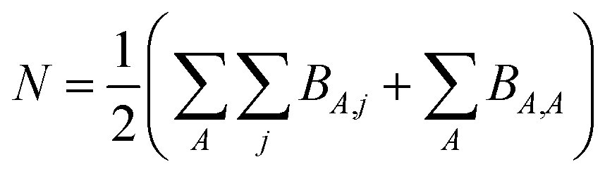
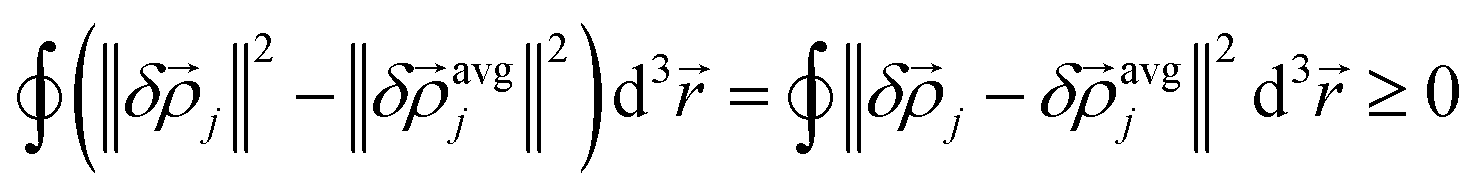
However, heuristic electron assignment can never approach universality, because it assigns bond orders in countable increments (e.g., whole numbers, half-numbers, one-thirds, etc.) while the bond order must properly be defined over the continuous set of non-negative real numbers. For a material containing N electrons in the unit cell, we can define a matrix BA,j that equals the number of electrons dressed-exchanged between an atom A in the reference unit cell and a particular atom j located anywhere in the material. Then,
 | (1) |
Equations analogous to eqn (1) hold for several chemical descriptors that partition the system's electrons into atom–atom pairwise components: (1) the atom–atom overlap populations,15 (2) the localization–delocalization matrix16 containing localization and delocalization indices,17,18 (3) bond orders computed using my comprehensive bond order equation, (4) the contact exchanges, and some others. The Laplacian bond index19 does not satisfy a normalization analogous to eqn (1). Except when the density matrices are idempotent, Mayer15,20 and Cioslowski21 bond indices do not satisfy a normalization analogous to eqn (1).18
The term “delocalization index” has sometimes been used to represent different things.22,23 For clarity, I use the terms second-order delocalization index (SODI), first-order delocalization index (FODI), Mayer bond index (MBI), and density-derived delocalization index (DDDI) to distinguish. Higher-order n-centered delocalization indices can be constructed from higher-order density matrices.24 The domain-averaged Fermi hole analysis of Ponec25 is related to delocalization indices and Ciosloski21 bond indices.
The SODI gets its name because it is a functional of the second-order density matrix. The SODI partitions the exchange–correlation (XC) hole, ρXC_hole(![[r with combining right harpoon above (vector)]](https://www.rsc.org/images/entities/i_char_0072_20d1.gif) ,′), into atom–atom pairwise components:
,′), into atom–atom pairwise components:
 | (2) |
|
fj() = ρj(j)/ρ()
| (3) |
that is assigned to atom j.17,26 Because the XC hole is a fundamental physical quantity closely related to the system's energy, the SODI should yield approximately consistent results across different correlated quantum chemistry methods27 and different SZ values of a spin multiplet. The SODI is computationally expensive, because it requires sixth-order integration of a function of and ′ in eqn (2). This can be re-written as the products of two three-dimensional integrals summed over the second-order density matrix components, but the large number of second-order density matrix components makes it expensive to compute and store.24 SODI measures something distinct from bond order.17 In some cases, SODI values approximately track bond orders, but in other cases SODI values and bond orders are quite different.17,22,27 For example, the SODI of N2 is ∼2.2–2.4 while this molecule has an ideal triple bond.17,22,27 Because it requires the second-order density matrix and is expensive to compute, the SODI will not be considered further here.
The FODI and MBI are functionals of the first-order density matrix.18,20 For atom A ≠ j,
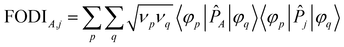 | (4) |
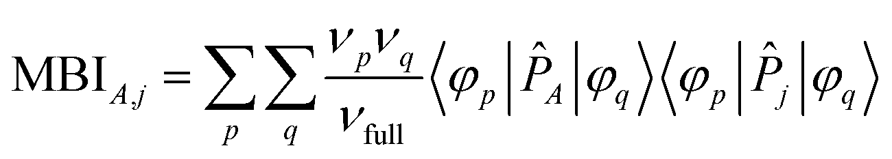 | (5) |
![[P with combining circumflex]](https://www.rsc.org/images/entities/i_char_0050_0302.gif) j is the atomic population analysis projector for atom j. The natural orbitals ({φp}) and their occupancies ({νp}) are the eigenvectors and eigenvalues, respectively, of the first-order density matrix. Different atomic population analysis schemes can be used to define the atomic projectors {j}: quantum chemical topology (e.g., QCT FODI and QCT MBI), natural population analysis (e.g., NAO MBI), Becke fuzzy partitioning (e.g., Fuzzy FODI and Fuzzy MBI), etc.15,22,28–30 For idempotent density matrices (i.e., all (νp/νfull) ∈ {0,1}), the FODI and MBI are equal. For a single-determinant Hartree–Fock calculation, the SODI, FODI, and MBI are equal.
j is the atomic population analysis projector for atom j. The natural orbitals ({φp}) and their occupancies ({νp}) are the eigenvectors and eigenvalues, respectively, of the first-order density matrix. Different atomic population analysis schemes can be used to define the atomic projectors {j}: quantum chemical topology (e.g., QCT FODI and QCT MBI), natural population analysis (e.g., NAO MBI), Becke fuzzy partitioning (e.g., Fuzzy FODI and Fuzzy MBI), etc.15,22,28–30 For idempotent density matrices (i.e., all (νp/νfull) ∈ {0,1}), the FODI and MBI are equal. For a single-determinant Hartree–Fock calculation, the SODI, FODI, and MBI are equal.
The DDDI is a new concept introduced in this article. The DDDI is an explicit functional of the electron and spin magnetization density distributions. Because it does not require computing basis function pair atomic overlaps, DDDI is easier to apply to large systems than SODI, FODI, and MBI. Across different types of quantum chemistry methods (e.g., DFT, coupled-cluster, and configuration interaction), DDDI yields more consistent agreement with conventional bond orders than SODI, FODI, and MBI. Because this article shows a DDDI based on DDEC6 partitioning can be constructed to give consistently accurate bond orders, the term DDEC6 bond order will be used here instead of DDEC6 DDDI.
2. Problems with prior computational approaches
Each computational bond index approach can be categorized by two criteria:(1) Whether it (A) can handle the general case of noncollinear spin magnetism or (B) requires electrons to be categorized as spin-up or spin-down (i.e., collinear spin magnetism).
(2) Whether it (A) is an explicit functional of the total electron density (ρ()) and spin magnetization density distributions, (B) explicitly depends on individual first-order density matrix components or eigenstates, (C) depends only on the system's geometry, or (D) explicitly depends on higher than first-order density matrices.
Category 1B cannot achieve universality, because it cannot describe noncollinear spin magnetism. As explained in the next paragraph, category 2B cannot achieve universality, because it exhibits unphysical dependence on the first-order density matrix representation. Category 2C, which depends only on the system's geometry, requires extensive empirical fitting. For example, bond-order-to-bond-length correlations can be developed for each pair of chemical elements,31 but this would require many empirically fitted parameters to cover the entire periodic table. To achieve high accuracy, bond-order-to-bond-length correlations would also need to incorporate other factors such as coordination number.32 Category 2D involves computationally expensive formulations, because of the high-order density matrices involved. Therefore, a computationally efficient universal first-principles approach to computing bond orders requires category 1A2A.
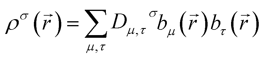
A universal method for computing bond orders cannot explicitly depend on individual first-order density matrix components or eigenstates. The first-order density matrix is related to the electron and spin densities by
 | (6) |
)} are the basis set functions. σ takes on one value for non-magnetism, two values for collinear magnetism, and four values for non-collinear magnetism. The density matrix eigenvectors are the natural spin orbitals, and its eigenvalues are the number of electrons (i.e., occupancies) in the natural spin orbitals. Two different density matrices can yield the same electron and spin magnetization densities and the same system energy, but different density matrix components and eigenstates. For example, a planewave basis set contains basis functions of the form  . If
. If ![[G with combining right harpoon above (vector)]](https://www.rsc.org/images/entities/i_char_0047_20d1.gif) (a) + (b) = (c) + (d) for some four basis functions (as is usually the case), then the electron density depends on Da,b + Dc,d but not individually on Da,b or Dc,d. However, the density matrix eigenstates depend on Da,b and Dc,d and not merely their sum. In the limit of a complete basis set, the density matrix components form an over-complete representation of the electron density distribution; that is, many different electron density matrices yield the same electron density distribution. A quantity that is a functional of the density matrix is thus not necessarily a functional of the electron density. At the zero of temperature, the density matrix for a nondegenerate density functional theory (DFT) state has only fully occupied and empty natural orbitals; that is, the density matrix eigenvalues are 0 or 1 for collinear magnetism and 0 or 2 for non-magnetism.33 In contrast, a correlated wavefunction that is N-representable is only required to have eigenvalues on the continuous interval [0,1] for collinear magnetism and [0,2] for non-magnetism.33,34 By the Hohenberg–Kohn theorems, the exact DFT and exact correlated wavefunction converge to the same electron density and energy.35 For spin-polarized materials, this was generalized to show the exact DFT and exact correlated wavefunction converge to the same electron density, spin magnetization density, and energy.36,37 Therefore, if a bond order method is constructed as a functional of the electron density matrix components or eigenstates, but not of the electron and spin magnetization distributions, it shall not necessarily yield same results for different quantum chemistry calculations even if those quantum chemistry calculations yield the same energy, electron density, and spin magnetization density. Such explicit dependence on irrelevant calculation details is completely unphysical.
(a) + (b) = (c) + (d) for some four basis functions (as is usually the case), then the electron density depends on Da,b + Dc,d but not individually on Da,b or Dc,d. However, the density matrix eigenstates depend on Da,b and Dc,d and not merely their sum. In the limit of a complete basis set, the density matrix components form an over-complete representation of the electron density distribution; that is, many different electron density matrices yield the same electron density distribution. A quantity that is a functional of the density matrix is thus not necessarily a functional of the electron density. At the zero of temperature, the density matrix for a nondegenerate density functional theory (DFT) state has only fully occupied and empty natural orbitals; that is, the density matrix eigenvalues are 0 or 1 for collinear magnetism and 0 or 2 for non-magnetism.33 In contrast, a correlated wavefunction that is N-representable is only required to have eigenvalues on the continuous interval [0,1] for collinear magnetism and [0,2] for non-magnetism.33,34 By the Hohenberg–Kohn theorems, the exact DFT and exact correlated wavefunction converge to the same electron density and energy.35 For spin-polarized materials, this was generalized to show the exact DFT and exact correlated wavefunction converge to the same electron density, spin magnetization density, and energy.36,37 Therefore, if a bond order method is constructed as a functional of the electron density matrix components or eigenstates, but not of the electron and spin magnetization distributions, it shall not necessarily yield same results for different quantum chemistry calculations even if those quantum chemistry calculations yield the same energy, electron density, and spin magnetization density. Such explicit dependence on irrelevant calculation details is completely unphysical.
In the past few decades, many approaches for computing bond orders from quantum chemistry calculations have been proposed, but all prior approaches lack sufficient chemical accuracy and universality. Bond index methods in category 1A2A include the Wheatley–Gopal38 and Laplacian19 overlap-to-bond-order correlations, but these have insufficient chemical accuracy because they incorrectly use constant bond-order-to-overlap ratios. Other bond index methods fall into categories that cannot achieve universality. Category 1A2B includes the MBI and FODI applied to overlapping (e.g., Fuzzy) or non-overlapping (e.g., QCT) density-based charge partitions.15,18,20,22,39 Bond order methods in category 1A2C include geometry-to-bond-order correlations.31,32 Category 1B2B includes natural bond orbital (NBO),40,41 natural localized molecular orbital (NLMO),42 adaptive natural density partitioning (ANDP),43,44 Ciosloski,21,45 MBI in the natural atomic orbital46 basis (NAO MBI),29 natural orbitals for chemical valence (NOCV),47 stockholder projector analysis48 and others; these methods produce localized orbitals that provide insights into orbital hybridization modes at the expense of inherent limitations for describing materials with delocalized bonding electrons. Because the NOCV and their associated Gopinathan–Jug49 (aka Nalewajski-Mrozek50) bond indices depend not only on individual density matrix components for the material of interest but also dramatically on somewhat arbitrary choice of reference fragments,50,51 they are not uniquely defined and so will not be computed in this article. Category 1A2D includes the SODI and multi-centered delocalization indices based on higher-order density matrices; these are computationally expensive.24
Only near equilibrium bond length is twice the bond order necessarily similar to the bonding orbital occupancies minus the antibonding orbital occupancies. This fundamental limitation arises, because as a bond is stretched the orbital occupancies and characters (e.g., bonding, antibonding, lone pair, lone valence) may change at a markedly different rate than electron exchanges between the two atoms. Consider the O2 molecule as an example. Near its equilibrium bond length, this molecule contains 1s core electrons; doubly occupied σ2s and 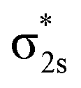 orbitals; doubly occupied σ2pz, π2px and π2py orbitals; and singly occupied
 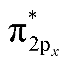 and
and 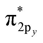 orbitals. As the O2 bond length is stretched beyond its equilibrium value, the orbital occupancies and their characters will remain similar until a critical point where they begin to suddenly change. In contrast, the exchange of electrons between the two atoms will smoothly decrease without a delay as the bond is stretched, because electrons of the second atom start moving away from the exchange holes of the first atom. Due to this fundamental mismatch in behaviors, stretched bond orders cannot be accurately computed via differences in bonding and antibonding orbital occupancies. This is true irrespective of the particular definition of bonding and antibonding orbitals. Consequently, all bond indices that first localize orbitals and then subtract antibonding orbital occupancies from bonding orbital occupancies do not accurately describe stretched bond orders.
Fig. 1 shows this for stretched O2 using intrinsic bonding orbitals52 (IBO) and natural localized molecular orbitals.42 The occupancy bond index (OBI) is defined as
| OBI = (∑(bonding orbital occupancies) − ∑(antibonding orbital occupancies))/2 | (7) |
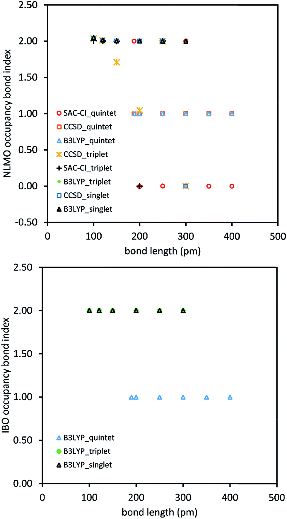 | ||
| Fig. 1 For stretched bonds, the bond order does not resemble the occupancy bond index. The NLMO and IBO occupancy bond indices for stretched O2 are shown in the top and lower graphs, respectively. The bond order should smoothly decrease towards zero as the bond length increases, but the occupancy bond indices do not produce this trend. | ||
Quantum chemistry calculations were performed for the O2 singlet, triplet, and quintet states at different bond lengths using the coupled cluster singles doubles (CCSD), symmetry adapted cluster configuration interaction (SAC-CI), and B3LYP exchange–correlation methods. These were then analyzed using 13 bond indices. The failure modes for each bond index were tallied and are reported in Table 1. Type 1 error fails occurred when a bond index assigned a difference ≥0.3 for the same geometry and spin multiplicity (i.e., singlet, triplet, or quintet) to results for different exchange–correlation methods (i.e., CCSD, SAC-CI, and B3LYP). For a given spin state, the bond order should change smoothly rather than abruptly with increasing bond distance. To quantify this effect, the ratio (BI(d))2/(BI(d+0.5 Å)*BI(d−0.5 Å)) was computed for each bond index (BI). This ratio (aka type 2 metric) is 1 for a purely exponential decay and close to 1 for other smooth curves that do not change abruptly. Type 2 error fails occurred when this type 2 metric was ≤½ or ≥2, which indicates the bond index versus bond distance curve changed abruptly. Type 3 error fails occurred when the bond index calculation failed to converge to any numeric value. Since ANDP is an extension of NBO to 2 or more bonding centers,43 its results for a diatomic (e.g., O2) molecule are identical to NBO.
| Method category | Type 1 error fails | Type 2 error fails | Type 3 error fails | |
|---|---|---|---|---|
| ANDP BI | 1B2B | 11/15 | 10/20 | 1/48 |
| Ciosloski BI | 1B2B | 6/8 | 2/10 | 15/48 |
| DDEC6 BO | 1A2A | 0/15 | 0/24 | 0/48 |
| DDEC6 CE | 1A2A | 0/15 | 0/24 | 0/48 |
| DDEC6 OP | 1A2A | 0/15 | 0/24 | 0/48 |
| Fuzzy FODI | 1A2B | 15/15 | 1/24 | 0/48 |
| Fuzzy MBI | 1A2B | 14/15 | 3/24 | 0/48 |
| Laplacian BI | 1A2A | 0/15 | 5/24 | 0/48 |
| NAO MBI | 1B2B | 14/15 | 5/24 | 0/48 |
| NBO BI | 1B2B | 11/15 | 10/20 | 1/48 |
| NLMO BI | 1B2B | 8/15 | 8/23 | 1/48 |
| QCT FODI | 1A2B | 15/15 | 3/24 | 0/48 |
| QCT MBI | 1A2B | 14/15 | 3/24 | 0/48 |
Each method that failed exhibited huge errors. For example, methods that failed via type 1 error exhibited max errors of 1.82 to 2.00 bond order. Also, these errors were not rare. Each method that failed at least one type 1 test failed more than 50% of type 1 tests. These failures were not caused by the choice of stretched O2 system, but rather by fundamental flaws of the failing methods. Specifically, all methods of category 2B exhibited pronounced type 1 errors, because this class of methods depends on specific density matrix components or eigenstates rather than being a functional of the electron and spin density distributions. Some methods that required orbital localization (i.e., ANDP, Cioslowski, NBO, NLMO) exhibited convergence failure (type 3 error) for at least one geometry. Overall, these results show prior bond indices fail frequently.
Fig. 2 plots DDEC6 bond order versus bond distance (d) for each O2 spin state. For the triplet, DDEC6 bond orders for SZ = 1 (CCSD) differed by less than 0.06 from those for SZ = 0 (SAC-CI) indicating a reasonably consistent treatment of these nearly degenerate spin states. For the quintet, DDEC6 bond orders for SZ = 2 (CCSD) differed by ≤0.10 from those for SZ = 0 (SAC-CI) indicating a reasonably consistent treatment of these nearly degenerate spin states. Because the DDEC6 bond order is a functional of the electron and spin densities, the CCSD and B3LYP results were reasonably consistent (max difference = 0.07).
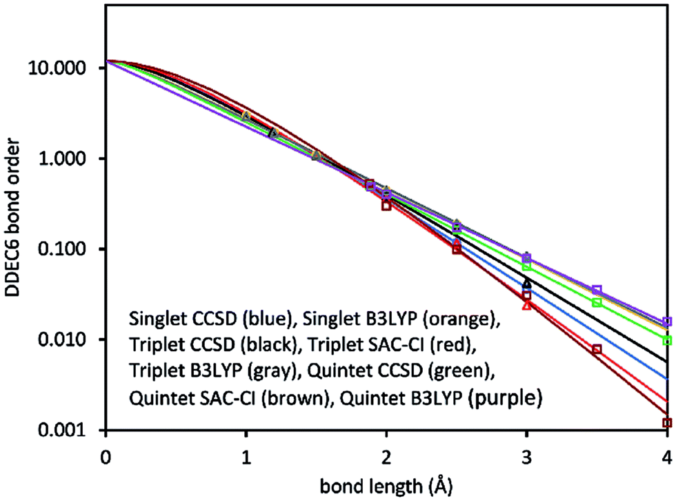 | ||
| Fig. 2 DDEC6 bond order versus bond length for the O2 molecule singlet (circles), triplet (triangles), and quintet (squares) spin states. The lines show the fitted model functions listed in Table 2. | ||
The computed data in Fig. 2 were fit to curves of the form
 | (8) |
Since the DDEC6 atomic electron distributions have exponentially decaying tails, and the DDEC6 bond orders roughly track the density overlaps between atoms, the DDEC6 bond orders decay exponentially with sufficiently large d. In the intermediate distances, DDEC6 bond orders can presumably have whatever behavior is required by the chemistry. Several studies showed SODI often exhibits sigmoidal shapes for covalent bond dissociation, exponential shapes for nonbonded interactions, and bell-shaped curves for charge-transfer.53 Eqn (8) fits the first two kinds of curves. Pauling showed the heuristic bond order for a specific pair of elements decays approximately exponentially with the equilibrium bond length.31
Pendas et al. argued SODI should decay exponentially with distance in gapped materials (e.g., semi-conductors and insulators) but algebraically in zero-gap materials (e.g., metallic conductors).54,55 If this is true, then DDEC6 bond orders and SODI exhibit much different decay laws in zero-gap materials. As shown in the Results and Discussion below, the DDEC6 SBOs accurately describe the number of bonding electrons per atom for a wide variety of material types, including conductors, semi-conductors, and insulators.
3. Theory
3.1 The dressed exchange hole
Bond order is not a direct experimental observable. The comprehensive bond order equation (eqn (22) below) expresses bond order in terms of a mathematical formula, but the various terms in this formula must be calculated rather than directly measured experimentally; therefore, bond order is not directly and unambiguously reducible to experimentally measured properties. For many systems, bond orders are correlated to some experimental properties (e.g., different bond lengths for a fixed element pair in organic molecules are correlated to bond order56), but such correlations fall short of a universal definition.If bond order is not a direct experimental observable, then how can we know whether a proposed definition is good or bad? One is not free to choose an arbitrary definition for bond order, because as shown in Sections 1 and 2 above many proposed definitions fail. This is analogous to deciding whether a proposed definition for a new standard unit is good or bad. Some considerations are: (a) how precisely can measurements be reproduced using a single method?57 (b) how precisely can measurements be reproduced using different methods?57 (c) is the new definition approximately in concert with prior definitions so it does not cause needless confusion?57 For example, the International System of Units has redefined the meter (unit of length) several times over the last few centuries, but always in such a way to make length measurements more reproducible while approximately in concert with the previous definition.57 Any definition with poor reproducibility can be discarded. The computed bond order should not be unduly sensitive to choice of basis set, exchange–correlation theory, or SZ value in a spin multiplet.
Mayer suggested bond order quantifies the number of electrons exchanged between two atoms in a material.20 Here, the term ‘exchanged’ refers to quantum mechanical exchange that occurs because an electron is a fermion. As shown in Section 2 above, MBI is not a functional of the electron and spin density distributions. Besides this limitation, there is another fundamental limitation. Consider the stretched [H2]+ system containing two atoms and one electron. When the two H atoms in this system are so far apart that the electron density in the middle is zero, then the electron density on the left side can be completely assigned to the left atom and the electron density on the right side can be completely assigned to the right atom. In this case, the MBI, FODI, SODI, and Cioslowki bond index are ½ for symmetric [H2]+ irrespective of how far apart the atoms are, and even if the atoms are infinitely far apart.
The uncertainty principle
 | (9) |
| (σx)intrinsic = h/(4πσp) | (10) |
When the bond length (d) is comparable to the intrinsic blurring in electron position (i.e., d ≈ (σx)intrinsic), then the electron inseparably belongs jointly to both atoms. When the bond length is much greater than the intrinsic blurring in electron position (i.e., d ≫ (σx)intrinsic), then the symmetric [H2]+ system can undergo quantum decoherence to yield either (a) H⋯[H+] or (b) [H+]⋯H. Such environmentally-induced decoherence of quantum superpositions is a well-established phenomenon.59 In this case, a measurement could yield the H+ cation on the left side or right side with equal probability, with the other atom being a neutral H atom. In the symmetry broken (a) or (b) systems or their symmetric quantum superposition, the bond order should arguably be zero, because the atoms are far apart and have non-overlapping electron distributions.
If we accept this argument that the bond order should be zero when atoms are so far apart that the electron density in the space between them is zero, then we must create a definition of bond order that is not a strict quantification of the number of electrons exchanged between two atoms. After the above argument involving the [H2]+ system, we might first be tempted to propose that bond order is a quantification of the number of electrons blurred between two atoms via the uncertainty principle. However, this definition is also insufficient, because its strict application would not necessarily produce bond orders close to the conventional values (e.g., ∼1 for H2, ∼3 for N2, etc.). Therefore, I decided to develop a more comprehensive definition of bond order.
From this argument, bond order quantifies some form of delocalization of electrons between atoms in a material, but this delocalization is neither strictly electron exchange nor strictly quantum blurring. Quantum blurring acts on indistinguishable particles. Specifically, indistinguishable particles are jointly blurred while distinguishable particles are independently blurred. In a multi-electronic system, some of the same-spin electrons are indistinguishable. Same-spin electrons undergo exchange. Therefore, it is the same-spin electrons that form the exchange and quantum blurring interactions leading to bond order. The delocalization of electrons leading to bond order can thus be described by a mathematical formalism resembling the exchange interaction, even though it is not strictly identical. Therefore, instead of partitioning the pure exchange hole among atoms to compute bond orders, we will instead partition a modified exchange hole (called the “dressed exchange hole”) to compute bond orders.
This dressed exchange hole is a modification of the pure exchange hole constructed for the sole purpose of computing bond orders. Like the pure exchange hole, the dressed exchange hole is constructed to exclude exactly one electron (eqn (S9) of ESI†). This dressed exchange hole may be constructed to be either more diffuse or more contracted than the pure exchange hole. If the atom-partitioned pure exchange hole integrates to larger (smaller) than accurate bond order, then we will construct the dressed-exchange hole to be more contracted (diffuse) than the pure exchange hole. Since making the hole more contracted (diffuse) decreases (increases) the calculated bond order, this modification makes the atom-partitioned dressed-exchange hole yield accurate bond orders. In cases where the atom-partitioned pure exchange hole already integrates to accurate bond order, then the dressed-exchange hole need not be more diffuse or contracted than the pure exchange hole.
This dressed exchange hole can incorporate the intrinsic quantum blurring associated with the uncertainty principle by setting the dressed exchange between two atoms A and j to zero when their DDEC6 atomic electron distributions (i.e., ρDDEC6A(A) and ρDDEC6j(j)) do not overlap. Specifically, the intrinsic quantum blurring of an electron belonging to atom A acts in the region of space where ρDDEC6A(A) > 0. If ρDDEC6A(A) and ρDDEC6j(j) overlap, then some of their electrons are indistinguishable, because they occupy the same spatial positions (i.e., the region of space where ρDDEC6A(A) and ρDDEC6j(j) overlap). Because some of their electrons are indistinguishable (i.e., shared), the bond order between atoms A and j is nonzero. If ρDDEC6A(A) and ρDDEC6j(j) do not overlap, then their electrons are distinguishable because they occupy distinguishable spatial positions. Because all of their electrons are distinguishable (i.e., not shared), the bond order between atoms A and j is zero in this case. Extending this argument, when the overlap between ρDDEC6A(A) and ρDDEC6j(j) is large (small), then the bond order between atoms A and j is also large (small).
In the ESI,† general mathematical properties of the dressed exchange hole are used to derive upper and lower bounds and scaling properties of the bond order. Actual construction and numerical integration of a dressed exchanged hole at every position in space would be computationally expensive, because this would require a six-dimensional integration over and ′ positions to yield the bond order. As described in Section S5 of ESI,† three of these integration dimensions are associated with property averaging. By using suitable algebraic correlations for property averaging over the dressed exchange hole, we can reduce the six-dimensional integration to a series expansion of three-dimensional integrations. As described in Section S6 of ESI,† a comprehensive bond order equation can be constructed that requires only three-dimensional integrations. This reduction from a six-dimensional integration over and ′ positions to three-dimensional integrations over positions is accurate, because it follows the derived upper and lower bounds and scaling properties of the bond order.
3.2 Summary of equations to compute comprehensive bond orders
In this article, a capital letter (e.g., A, B, etc.) will be used to represent an atom in the reference unit cell while atoms anywhere in the material will be represented by small letter indices (e.g., j). In a periodic material, atom j is labeled by (B,![[small script l]](https://www.rsc.org/images/entities/char_e146.gif) 1, 2, 3), where B is an atom in the reference unit cell and 1, 2, and 3 are the translation whole numbers along the lattice vectors
1, 2, 3), where B is an atom in the reference unit cell and 1, 2, and 3 are the translation whole numbers along the lattice vectors ![[v with combining right harpoon above (vector)]](https://www.rsc.org/images/entities/i_char_0076_20d1.gif) 1, 2, and 3, respectively, to give the nuclear position
1, 2, and 3, respectively, to give the nuclear position
![[R with combining right harpoon above (vector)]](https://www.rsc.org/images/entities/i_char_0052_20d1.gif) j = B + 11 + 22 + 33 j = B + 11 + 22 + 33
| (11) |
B is the nuclear position of atom B. For a non-periodic material, the vectors 1, 2, and 3 can be chosen to define any parallelepiped completely enclosing the electron distribution. In non-periodic materials, 1 = 2 = 3 = 0 for all atoms. In materials having one periodic dimension, 2 = 3 = 0 for all atoms. In materials having two periodic dimensions, 3 = 0 for all atoms.|
j = − j
| (12) |
j) to position . rj = ‖j‖ is the distance from atom j's nuclear position to position . The condition j ≠ A means that j ≠ A.
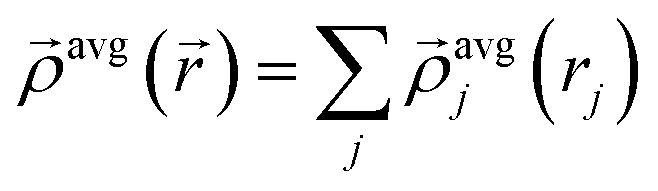
To construct a comprehensive bond order, the first step is to express the atomic exchange propensity (i.e., the tendency of each atom to exchange electrons with other atoms) as functionals of {ρ(),![[m with combining right harpoon above (vector)]](https://www.rsc.org/images/entities/i_char_006d_20d1.gif) ()}, where () is the spin magnetization density vector that handles either collinear or non-collinear magnetism. To each atom j is assigned an atomic electron density ρj(j) and an atomic spin magnetization density vector j(j) that are combined to form the four-vector
()}, where () is the spin magnetization density vector that handles either collinear or non-collinear magnetism. To each atom j is assigned an atomic electron density ρj(j) and an atomic spin magnetization density vector j(j) that are combined to form the four-vector
![[small rho, Greek, vector]](https://www.rsc.org/images/entities/i_char_e137.gif) j(j) = (ρj(j),j(j)) j(j) = (ρj(j),j(j))
| (13) |
|
avgj(rj) = (ρavgj(rj),avgj(rj))
| (14) |
j(j) over the exchange hole and (b) a weighted average of avgj(rj) over the exchange hole. Here, this is called the confluence of atomic exchange propensities. From the basic identity
 | (15) |
j is more sensitive than avgj to changes in the basis set, exchange–correlation theory, and charge and spin partitioning algorithm. Therefore, more stable results will occur if the atomic exchange propensity is based on avgj(rj) rather than on j(j).
We begin by defining the contact exchange CEA,j for A ≠ j as the electron exchange that would occur between atoms A and j if the (modified) exchange hole centered around each position were a Dirac delta function that integrates to 1 but has negligible radius:
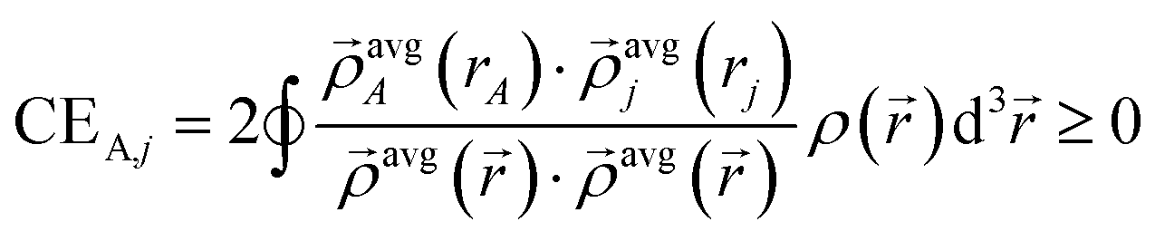 | (16) |
 | (17) |
 | (18) |
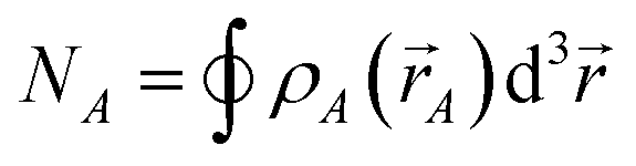
| CEA,A = NA − ½SCEA | (19) |
 | (20) |
As derived in Sections S2–S4 of ESI,† the ratio of bond order to contact exchange for an atom pair is bound by
| 1 ≲ ΦA,j = (BA,j/CEA,j) ≲ 2 | (21) |
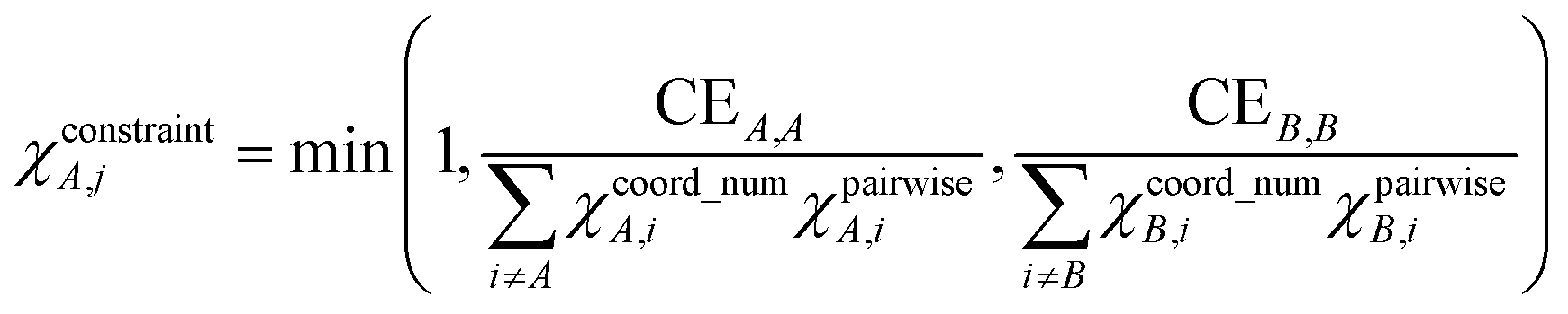
| BA,j = CEA,j + χcoord_numA,jχpairwiseA,jχconstraintA,j = CEA,j + ΛA,j | (22) |
is in fact not a Dirac delta function but has a non-negligible spatial extent. ΛA,j equals the product of (a) χpairwiseA,j accounting for pairwise interactions, (b) χcoord_numA,j accounting for coordination number effects, and (c) χconstraintA,j that imposes a constraint on the density-derived localization index (DDLI) BA,A. As derived in Section S6 of ESI,† eqn (22) is unique, because it has the simplest mathematical form capable of accurately describing the primary bond order effects.
The contact-exchange-weighted coordination number
 | (23) |
| χcoord_numA,j = 1 − (tanh((CA + Cj − 2)/K3))2 | (24) |
The pairwise term is given by
| χpairwiseA,j = min(ΩA,j,CEA,j) | (25) |
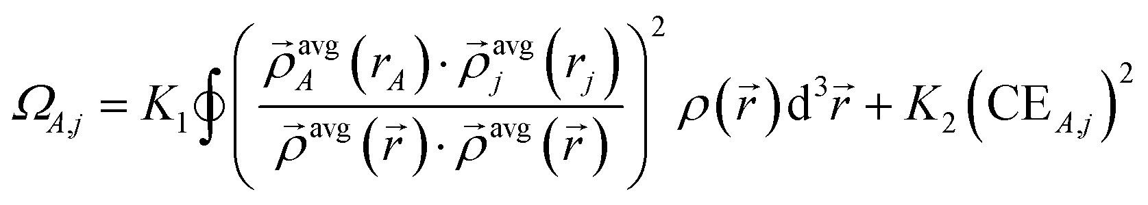 | (26) |
The parameters
 | (27) |
The sum of bond orders (SBO) for atom A is
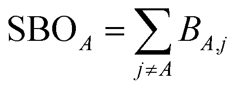 | (28) |
 | (29) |
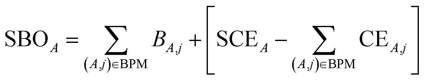
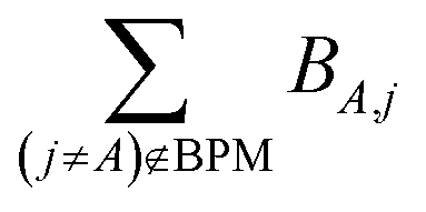 for those atom pairs not included in the bond pair matrix. In such a way, eqn (29) computes SBOA including all atom pairs j ≠ A, not just those included in the bond pair matrix. For the presently chosen cutoffs (i.e., bond_print_threshold = 0.001 and cutoff_radius = 5 Å), the bracketed term in eqn (29) is nearly always <0.02, because the system geometry typically only allows a few dozen atoms j to be only slightly outside the cutoff criteria for inclusion of (A,j) in the bond pair matrix and atoms j well outside the inclusion cutoff criteria will contribute negligibly to SBOA.
The DDLI of atom A is found by
| BA,A = NA − ½SBOA | (30) |
| 2BA,A ≥ CEA,A ≥ BA,A ≥ 0 | (31) |
 | (32) |
Fig. 3 concisely illustrates relationships between key equations used to compute DDEC6 bond orders. Blue text annotations explain key terms in each equation. Arrows indicate the sources of information used in each equation. These arrows show which equations are used to compute quantities used in other equations. Each variable reappearing in several different equations is marked with a specific color of squiggly underline (note: sometimes a variable reappears inside a summation). Red boxes enclose the main equation and key concepts. These key concepts act as the source of information for some equations.
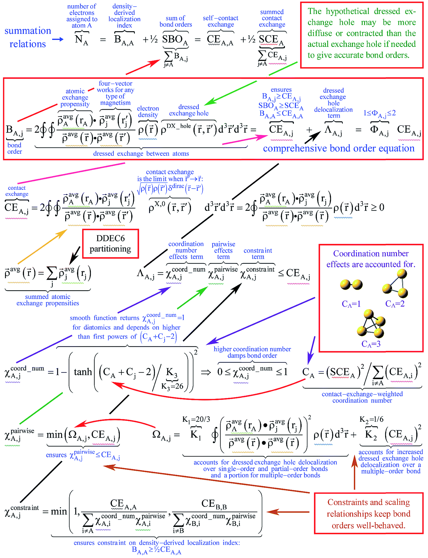 | ||
| Fig. 3 Diagram showing key relationships between equations for computing DDEC6 bond orders. Red boxes enclose the main equation and high level concepts. Arrows indicate the sources of selected inputs or concepts used in each equation. Each variable reappearing in several different equations is marked with a specific color of squiggly underline (note: sometimes a variable reappears inside a summation). Blue text annotations explain key terms. | ||
To better understand constraint (31), consider the bond order versus bond length (d) curve for a homodiatomic molecule AB. In the hypothetical d → 0 limit, both atoms become equivalent because they have the same nuclear position and atomic number (such a limit is purely hypothetical, because in a real scenario the atoms might undergo a nuclear fusion reaction). In this limit, ρavgA(rA) = ½ρavg() for all . This gives CEA,A = CEB,B = ½CEA,B = ¼N = ½NA, where N is the total number of electrons. From eqn (31) it directly follows that ¼NA ≤ BA,A ≤ ½NA in this limit. Finally, from eqn (30) it directly follows that NA ≤ SBOA = BA,B ≤ (3/2)NA in this limit. Because CEA,B becomes large in the d → 0 limit, the quadratic term in eqn (26) causes BA,B to approach the upper limit of (3/2)NA. Even though such a limit is purely hypothetical, it tells us the d → 0 intercept of the bond order versus bond length curve for a homodiatomic molecule is p1 = (3/2)NA. For d > 0, CEA,B decreases causing BA,B < (3/2)NA for a homodiatomic molecule at physically realizable bond lengths.
If we roughly interpret the historical idea of bond order as the number of “electron pairs” “shared” between two atoms, then the maximum physically realizable bond order in a homodiatomic molecule would be BA,B ≈ NA, because there are N = 2NA electrons in the material. One should be cautious about this conventional notion of bond order, because it does not strictly hold in the d → 0 limit. In the d → 0 limit of a diatomic molecule, the comprehensive bond order equation gives BA,B → (3/2)NA which is 1.5 times the number of electron pairs. This behavior results from two factors. First, for the singlet H2 molecule near its equilibrium bond length the computed bond order should be ∼1 to achieve approximate backwards compatibility with the historical notion of bond order. Second, for optimal chemical relevance, when using an overlapping atoms paradigm (e.g., DDEC6 partitioning as opposed to QCT's non-overlapping compartments) the bond order should increase as atomic density overlaps increase. Because the density overlap between overlapping H atoms in H2 increases as bond length decreases, the computed bond order exceeds 1 (the number of electron pairs) for singlet H2 at highly compressed bond lengths. Thus, either we have to relax the notion of bond order as being a strict quantification of “electron pairs” or we have to relax the notion of bond order as being sensitive to atomic density overlaps. Because a chemical bond can be formed without pairing any electrons (e.g., [H2]+), the choice is easy.
As examples, DDEC6 bond order versus bond length is plotted in Fig. 4 for the H2 singlet and triplet and [H2]+ doublet. [H2]+ shows chemical bonding can be achieved even by a single electron. For all three molecules, the bond orders smoothly decrease with increasing bond length. The data was fit to the model curve of eqn (8). The fitted parameters for these systems and the stretched O2 systems (Fig. 2) are listed in Table 2. The squared correlation coefficients >0.99 indicate the model described the data well.
 | ||
| Fig. 4 DDEC6 bond order versus stretched bond length for the H2 singlet, H2 triplet, and [H2]+ doublet spin states. The lines show the fitted model functions listed in Table 2. | ||
| Molecule | Spin state | XC theory | p1 | p2 (Å−1) | p3 (Å) | Squared correlation coefficient |
|---|---|---|---|---|---|---|
| [H2]+ | Doublet | Exact | 0.75 | 1.4687 | 1.2104 | 0.9915 |
| H2 | Singlet | Exact | 1.5 | 2.0284 | 1.9089 | 0.9993 |
| H2 | Triplet | Exact | 1.5 | 1.6708 | 0.7712 | 0.9982 |
| O2 | Singlet | CCSD | 12 | 2.3951 | 0.7304 | 0.9995 |
| O2 | Singlet | B3LYP | 12 | 1.8095 | 0.2287 | 0.9987 |
| O2 | Triplet | CCSD | 12 | 2.1866 | 0.5653 | 0.9950 |
| O2 | Triplet | SAC-CI | 12 | 2.7481 | 1.0708 | 0.9958 |
| O2 | Triplet | B3LYP | 12 | 1.7844 | 0.2031 | 0.9985 |
| O2 | Quintet | CCSD | 12 | 1.8591 | 0.1954 | 0.9999 |
| O2 | Quintet | SAC-CI | 12 | 3.2094 | 1.7067 | 0.9934 |
| O2 | Quintet | B3LYP | 12 | 1.6720 | 0.0000 | 0.9988 |
Garcia-Revilla et al. reported SODI curves for H2 singlet and triplet.53 With minor differences, the shapes of the H2 singlet and triplet curves are roughly similar for the DDEC6 bond order compared to the SODI. However, the triplet state is farther below the singlet state for the SODI53 than for the DDEC6 bond order. In contrast, for [H2]+ the SODI is constant at 0.5 irrespective of the bond length, while the DDEC6 bond order decreases smoothly with increasing bond length. A different kind of bonding analysis, called the electron delocalization range (EDR), has been reported for stretched H2 singlet and [H2]+.60 EDR quantifies electron distance profiles rather than bond orders, and it is hard (not intuitive) to interpret.60
3.3 Choice of charge and spin partitioning method
An appropriate charge and spin partitioning method must be used to compute the bond orders defined by eqn (22). Obviously, the assigned {ρj(j)} and {j(j)} must sum to ρ() and () at each position . To be chemically feasible, the assigned spin magnetization density is bound by:|
0 ≤ ‖A(A)‖ ≤ ρA(A)
| (33) |
|
ρavgA(rA) ≈ ρA(A) ≈ real atom
| (34) |
 | (35) |
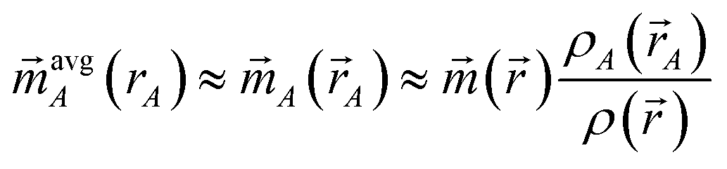
The electron distribution assigned to each atom should have features resembling a real atom. Specifically, the tail of ρavgA(rA) should decay approximately exponentially with increasing rA, and the assigned ρavgA(rA) should be neither too diffuse nor too contracted. To meet the condition that assigned bond orders for nearly degenerate spin states (e.g., SZ = 0 and SZ = ±1 triplet states) are nearly equal: (i) the assigned A(A) should resemble proportional spin partitioning as defined on the right-hand side of eqn (35) and (ii) the assigned {ρA(A)} should be a functional of {ρ()} alone without depending on {()}.
The following stockholder charge partitioning methods are suboptimal for use with the comprehensive bond order equation, because they fail to satisfy some of these requirements: Hirshfeld (H),61 Hirshfeld Iterative (HI),62 Iterative Stockholder Atoms (ISA),63 Fractionally Occupied Hirshfeld Iterative (FOHI),64 Gaussian Iterative Stockholder Atoms (GISA),65 Hirshfeld Extended (HE),66 basis space iterative stockholder atoms with density fitting (BS-ISA+DF),67 and Minimal Basis Iterative Stockholder (MBIS).68,69 The H, HI, FOHI, and HE methods do not specifically optimize ρA(A) to resemble ρavgA(rA). The ISA and GISA methods do not specifically optimize the tail of ρavgA(rA) to decay approximately exponentially with increasing rA. The H, HI, ISA, FOHI, GISA, HE, BS-ISA+DF, and MBIS methods lack constraints to prevent buried atoms from becoming too diffuse or too contracted. The FOHI assigned {ρA(A)} depend on both the electron and spin density distributions rather than being a functional of {ρ()} alone.64 Sometimes, the HI (and by extension FOHI) methods do not converge to a unique solution.70 The H method often underestimates the net atomic charge (NAC) magnitudes,71 while the HI method often overestimates them.72 The ISA, GISA, and HE methods exhibit poor chemical or conformational transferability.65,68,73
The DDEC6 charge partitioning method of Manz and Gabaldon Limas70,74 is well-suited for computing bond orders, because DDEC6 is optimized to satisfy all of the requirements listed here.70,74 The DDEC6 charge partitioning method simultaneously optimizes ρA(A) to resemble ρavgA(rA) and a charge-compensated reference ion of the same chemical element in a similar (but not necessarily identical) charge state.70,74 It uses constraints to prevent the assigned {ρA(A)} from becoming too diffuse or too contracted.70,74 Moreover, the number of electrons assigned to each atom in the material is optimized to resemble the number of electrons in the volume dominated by each atom, which greatly improves the accuracy of describing charge transfer in materials.70,74 DDEC6 uses the spin partitioning method of Manz and Sholl,75 which optimizes the assigned atomic spin magnetization density (A(A)) to simultaneously resemble its spherical average (avgA(rA)) and proportional spin partitioning (right side of eqn (35)) subject to constraint (33). DDEC6 is computationally efficient and always converges to a unique solution in seven charge partitioning steps (i.e., a small number of iterations).70 Moreover, DDEC6 is the only partitioning method published to date that meets all of these requirements. The DDEC6 method provides exceptionally accurate charge and spin partitioning across an extremely diverse range of material types.70,74
The relationship between DDEC6 partitioning and the confluence of atomic exchange propensities is summarized in Fig. 5. There are three main reasons for using the confluence of atomic exchange propensities. First, good spatial transferability of the atomic exchange propensities is required, because the exchange interaction occurs over the exchange hole around each position . Since contours of constant rA pass through more points in the exchange hole than A does, avgA(rA) may be a better choice than A(A) to represent the atomic exchange propensity. Second, as shown in Section 5.3 below, the atomic exchange propensities should be similar to proportional spin partitioning to produce similar bond orders for different SZ values of a spin multiplet. Third, as derived in eqn (15) above, using avgA(rA) instead of A(A) reduces sensitivity to the choice of exchange–correlation theory, basis sets, and charge partitioning method. Together, these imply the atomic exchange propensities should be simultaneously optimized to resemble proportional spin partitioning, spherical averaging of charge, and spherical averaging of spin. As illustrated at the bottom of Fig. 5, the DDEC6 method does this.
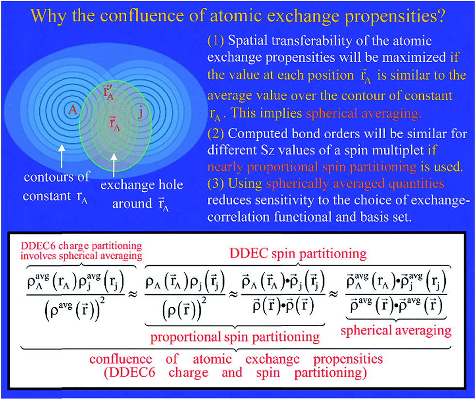 | ||
| Fig. 5 Graphic explaining why the confluence of atomic exchange propensities is important and its relationship to DDEC6 charge and spin partitioning. | ||
The method does not apply to electrides, nuclear reactions, highly time-dependent states, and some extremely high-energy excited states. An electride is a material containing an electron as the anion.76 Because the DDEC6 method assigns all electron density to atoms, it is not optimal for studying electrides.70 Because the structures of atomic nuclei are assumed to be conserved during DDEC6 analysis, nuclear reactions also fall outside the scope of DDEC6 analysis. The method is also not applicable to highly time-dependent states when a state evolves so rapidly the orbiting electrons do not have time to approximately equilibrate with the nuclear motions. Finally, extremely high-energy excited states fall outside the scope of the DDEC6 method when they have atomic electron densities dramatically different from the reference ions used in the DDEC6 method. For example, excitations producing core electron vacancies are not well-described, because the currently available DDEC reference ions have no core electron vacancies. The method could potentially be extended to excited states with core electron vacancies by modifying the DDEC reference ions to include corresponding core electron vacancies, but this has not been tested.
4. Methods
4.1 Materials selection
The set of materials contained at least one element from each chemical group (i.e., groups 1–18, lanthanides, actinides, and transactinides) and at least one element from each periodic row (i.e., rows 1–7). The materials were chosen to include a wide range of bonding motifs: ionic, covalent, polar-covalent, metallic, electron deficient multi-center, hypercoordinate, aromatic, agostic, opportunistic, Lewis acid–base, multi-reference, dispersion, and hydrogen bonding. A wide range of material types were included: inorganic molecules, a biomolecule, organometallic complexes, ions, porous solids, nonporous solids (electrically conducting, semiconducting, and insulating), a solid surface, a polymer, sheets, nanoclusters, and an endohedral complex. In addition to ground state geometries, some transition states, and non-equilibrium geometries were included. Materials were included with no magnetism, collinear magnetism, and non-collinear magnetism. Different spin states were considered for some of the magnetic structures. Materials were also included to span a wide range of bond orders from nearly zero to quadruple bond.Individual materials were selected according to their familiarity, novelty, and computational availability. The stretched O2 molecule was selected for comparing computed bond indices, because O2 is a classic textbook example of bond order via a molecular orbital diagram.6,77 The diatomic molecules were chosen to include both common (e.g., halogen dimers, halogen acids, H2, O2, N2, NO, CO, etc.) and novel (e.g., Be2, Kr2, U2, etc.) entries spanning a wide range of bond orders. The U2 molecule was included, because its bonding properties were previously studied using high-level quantum chemistry calculations.78 The pure transition metal solids were selected, because they are a classic example of metallic bonding.6 Diborane (B2H6) was selected as a classic textbook example of an electron deficient molecule with multicenter bonding.6 SF6 was selected as a classic example of a hypercoordinate molecule.79 The Fe4C40H52N4O12 single molecule magnet was chosen as an example of non-collinear magnetism, because its DFT-optimized geometry and electron and spin magnetization distributions were already available75 (optimizing non-collinear magnetism structures is extremely difficult and time-consuming75). The ethylene polymerization transition state was chosen because it demonstrates agostic bonding and several bonds in an intermediate state between reactant and product. The biomolecule was chosen through a careful query of the Protein Data Bank to identify crystal structures of proteins containing a couple hundred atoms that have the positions of all hydrogen atoms refined without any disordered atoms. Only a few structures met this criterion. PDB entry 1ETM containing 160 non-solvent atoms was selected, because its resolution (0.89 Å), R-value work (0.065), clashscore (0), Ramachandran outliers (0), and sidechain outliers (0) indicate the crystal structure has been refined to exceptionally high fidelity.80 Diamond, silicon, graphite, graphene, boron nitride, and ice crystal structures were selected, because they are widely researched materials. The remaining materials were selected to highlight additional types of systems and bonding motifs.
4.2 Quantum chemistry methods
All quantum chemistry calculations in this article used the Born-Oppenheimer approximation. The Born–Oppenheimer approximation treats the electronic and nuclear motions as separable.81 This approximation is reasonable, because of the large differences in masses between electrons and atomic nuclei.81 The bond order method described in this article is only applicable to time-independent and modestly time-dependent states where the Born–Oppenheimer approximation is reasonable. Highly time-dependent states where the Born–Oppenheimer approximation fails are not suitable for use with this bond order method.Table 3 lists computational details for each material studied. For each material, the spin state, exchange–correlation (XC) method, basis set, and electron treatment are listed. CS and OS denote closed-shell and open-shell singlets, respectively. The electron treatments are: (a) fully relaxed non-relativistic all-electron (AE) calculation, (b) relativistic frozen core (RFC) that uses a scalar relativistic correction for valence electrons and high-level relativistic frozen core electrons, (c) fully relaxed relativistic all-electron (RAE) calculation using 4th order Douglas–Kroll–Hess method with spin–orbit coupling (GAUSSIAN 09 keyword DKHSO which includes a finite-size Gaussian nuclear model82), (d) non-relativistic relaxation of valence electrons and replacement of core electrons with a relativistic effective core potential (RECP), and (e) non-relativistic all-electron calculation freezing some core electrons during the electron correlation calculation (FC). Some calculations marked as RECP used RECP on the heavier atoms but all electrons on the lighter atoms. For each material, the geometry type (experimental, optimized, transition state, constrained, or increments) is also listed. The literature references for each geometry and electron density distribution are also listed.
| System | Spin (S) | XC method | Basis set | Electron treatment | Geometry type | Geometry reference | Density reference |
|---|---|---|---|---|---|---|---|
| a MUGBS on Db and aug-cc-pvqz on F atoms.b Geometry optimized but constrained to octahedral symmetry.c Since the experimental hexagonal ice crystal contains many fractionally occupied H atom sites,95 the geometry for electron density generation had to choose an appropriate fraction of these to populate with actual H atoms.d The ice surface geometry is a slab with several ice layers (extracted from the ice crystal structure) followed by >10 Å vacuum space.e AE for CCSD and FC for SAC-CI.f The CISD method for a two-electron system (e.g., stretched H2) is an exact full configuration interaction calculation.g AE except RECP on Rb, Te, I, and Cs.h The HF calculation for a one-electron (e.g., stretched [H2]+) system is an exact exchange–correlation calculation.i AE except RECP on Te. | |||||||
| 1ETM | 0 (CS) | PBE | Planewave | RFC | Experiment | 80 (solvent removed) | This work |
| B2H6 | 0 (CS) | PW91 | 6-311++G** | AE | Optimized | This work | This work |
| B4N4 | 0 (CS) | PW91 | 6-311++G** | AE | Optimized | 72 | 72 |
| BN nanotube | 0 (CS) | PW91 | Planewave | RFC | Optimized | 72 | 72 |
| BN sheet | 0 (CS) | PBE | Planewave | RFC | Optimized | 74 | 74 |
| [DbF6]− | 0 (CS) | PBE | a | RAE | Constr. opt.b | This work | This work |
| [Eu@C60]+ | 4 | PBE | Planewave | RFC | Optimized | 70 | 70 |
| Graphene | 0 (CS) | PBE | Planewave | RFC | Optimized | This work | This work |
| H3N·BF3 | 0 (CS) | PBE | 6-311++G** | AE | Optimized | This work | This work |
| Ice crystal | 0 (CS) | PBE | Planewave | RFC | Experiment | c | This work |
| Ice surface | 0 (CS) | PBE | Planewave | RFC | Experiment | d | This work |
| Na3 | ½ | PBE+D3 | aug-cc-pvtz | AE | Optimized | This work | This work |
| Fe4O12N4C40H52 | Noncollinear | PW91 | Planewave | RFC | Optimized | 75 | 75 |
| Organomet. cation | 0 (CS) | OLYP | 6-311++G** | AE | Optimized | 89 | 89 |
| Cu3BTC2 MOF | 0 (OS) | PW91 | Planewave | RFC | Optimized | 90 | 90 |
| Diamond, Si, NaF, and NaCl solids | 0 (CS) | PBE | Planewave | RFC | Optimized | This work | This work |
| Graphite | 0 (CS) | PBE | Planewave | RFC | Experiment | 91 | This work |
| h-BN solid | 0 (CS) | PBE | Planewave | RFC | Experiment | 92 | This work |
| Li, Na, & K solids | 0 (CS) | PBE | Planewave | RFC | Optimized | This work | This work |
| Natrolite | 0 (CS) | PBE | Planewave | RFC | Optimized | 73 | 73 |
| Ozone | 0 (CS) | CAS-SCF | aug-cc-pvtz | FC | Optimized | 72 | 72 |
| Polyfluoroprene | 0 (CS) | PBE | 6-311++G** | AE | Optimized | This work | This work |
| SF6 | 0 (CS) | M06L | aug-cc-pvtz | AE | Optimized | This work | This work |
| Silylene | 0 & 1 | CCSD & SAC-CI | aug-cc-pvtz | e | Optimized | This work | This work |
| Stretched H2 | 0 & 1 | Exactf | aug-cc-pvqz | AE | Increments | This work | This work |
| Stretched O2 | 0, 1, & 2 | CCSD, SAC-CI, & B3LYP | daug-cc-pvqz | AE | Increments | This work | This work |
| [H–H–F] | ½ | CCSD | aug-cc-pvtz | FC | Transition state | 93 | 93 |
| Polymerization chain initiation | 0 (CS) | OLYP | LANL2DZ | RECP | Transition state | 94 | 94 |
| 26 diatomics | Various | PBE | MUGBS | RAE | Optimized | This work | This work |
| 23 diatomics | Various | CCSD | def2qzvppd | g | Optimized | This work | This work |
| U2 | 3 | CCSD | Largecore SDD | RECP | Optimized | This work | This work |
| Stretched [H2]+ | ½ | Exacth | def2qzvppd | AE | Increments | This work | This work |
| Be2 | 0 (CS) | SAC-CI | def2qzvppd | FC | Optimized | This work | This work |
| S2, Se2, & Te2 | 1 | SAC-CI | def2qzvppd | i | Optimized | This work | This work |
| 20 pure transition metal solids | Various | PBE | Planewave | RFC | Optimized | This work | This work |
All planewave quantum chemistry calculations were performed using the Vienna ab initio simulation package (VASP). VASP uses the projector augmented wave (PAW83,84) method to represent each chemical element using an all-electron relativistic frozen-core method.85,86 In each case, the PAW for the corresponding exchange–correlation functional (PBE87 or PW91 (ref. 88)) was used. The planewave cutoff energy, k-point mesh, and orbital occupancy smearing parameters were chosen to achieve results effectively converged near the complete basis set limit. A planewave cutoff energy no smaller than 400 eV was used for each material. The k-point mesh was chosen so the product of number of k-points times the unit cell volume was at least 4000 Å3; this corresponds to the number of k-points along each lattice direction times the lattice vector length being at least 16 Å. For the pure transition metal solids, the presented results correspond to: (a) a planewave cutoff energy of 750 eV, (b) the number of k-points along each lattice direction times the lattice vector length being at least 32 Å, (c) a fermi smearing parameter value of 0.05 eV, (d) forces on each atom converged to within 0.01 eV Å−1, (e) electronic energy converged to within 10−5 eV, and (f) using the PAW potentials recommended on the VASP website. For the pure transition metal solids, additional tests showed that reducing the planewave cutoff energy to 400 eV, reducing the k-point mesh so the product of number of k-points times the unit cell volume was ∼4000 Å3, and using fewer number of valence electrons in the PAW potential (i.e., larger number of frozen core electrons) led to no appreciable differences in results. Therefore, the results can be considered converged near the complete basis set limit.
For molecules, a variety of exchange–correlation methods and basis sets were used to demonstrate the feasibility of computing useful bond orders from different levels of theory. All quantum chemistry calculations using Gaussian basis sets were performed in the GAUSSIAN 09 software.96 Basis sets of at least triple zeta quality with added polarization and diffuse functions were used in all cases except the polymerization chain initiation transition state (LANL2DZ basis set) and the uranium dimer CCSD calculation (largecore SDD basis set) for which calculations converged only using smaller basis sets. The 6-311++G**, LANL2DZ, aug-cc-pvtz, aug-cc-pvqz, and daug-cc-pvqz basis sets were included in GAUSSIAN 09.96 The def2qzvppd and SDD basis sets were obtained from the EMSL basis set exchange.97,98 The SDD basis set used for the uranium dimer CCSD calculation had a RECP that replaced 78 core electrons. The LANL2DZ basis set used a RECP to replace 10 (Ti) and 28 (Br) core electrons. The def2qzvppd basis set used a RECP to replace 28 (Rb, Te, I) and 46 (Cs) core electrons. All other calculations were all-electron. The MUGBS basis set is the universal Gaussian basis set from Manz and Sholl that has the same form for every chemical element.72 MUGBS yields atomic population results near the complete basis set limit. Different DFT methods used included pure, meta, hybrid, and dispersion-corrected functionals: OLYP,99 PBE,87 M06L,100 B3LYP,101,102 and PBE with Grimme's D3 dispersion correction103 (PBE+D3). Two coupled-cluster methods were used: CCSD104 and SAC-CI.105,106 Two configuration interaction methods were used: CAS-SCF107 and CISD.108
DDEC6 bond order analysis was programmed into the CHARGEMOL program. DDEC6 analysis is always performed using an effective all-electron density.70 In cases where a frozen core was used in the quantum chemistry calculation (e.g., VASP PAW results), the frozen core electrons were included in the DDEC6 analysis.70 In cases where a RECP was used in the quantum chemistry calculation, the core electrons replaced by the RECP were added back in at the start of DDEC6 analysis.70
For stretched O2, other bond indices were computed using the following software programs. NBO and natural population analysis (NPA) were performed using the NBO 6 program.109,110 The NBO keywords BNDIDX RESONANCE NLMO were included in the analysis. The NBO bond index was computed by subtracting the anti-bonding NBO populations from the bonding NBO populations and then dividing by two (eqn (7)). Because the NAOs computed during NPA are orthonormal, the MBI in the NAO basis (i.e., NAO MBI) equals the spin-resolved Wiberg bond index printed by the NBO 6.0 program. The NLMO occupancy bond index was also printed by the NBO 6.0 program.
The Laplacian bond index, Fuzzy FODI, QCT FODI, Fuzzy MBI, and QCT MBI were computed using the MultiWFN111 program. With the following minor modifications, the wfx file output from GAUSSIAN 09 was used as the input to the MultiWFN program. Since the FODI used the square roots of natural orbital occupancies (eqn (4)), any natural orbital occupancies less than zero were changed to zero. This was only a minor adjustment, because such occupancies were already close to zero. Very high quality integration grids were used for all of the MultiWFN calculations. The Fuzzy FODI and Fuzzy MBI were computed using MultiWFN's default atomic radii and k = 3 value for Becke112 electron density partitioning. As shown in eqn (4) and (5), the FODI and MBI have analogous mathematical forms, except the FODI uses the product of square roots of two natural orbital occupancies while the MBI uses the product of two natural orbital occupancies divided by νfull. To compute the Fuzzy MBI and the QCT MBI, a second wfx file was prepared in which the natural orbital occupancies were squared and divided by νfull; this resulted in the recovery of the MBI formula when the square roots were taken. This tricked the MultiWFN program into computing the Fuzzy MBI and the QCT MBI from the Fuzzy FODI and QCT FODI routines, respectively.
Cioslowski's covalent bond index was computed in GAUSSIAN 09.21,96 Because Cioslowski's covalent bond index did not converge when using the daug-cc-pvqz basis set, the CEP-121G* basis set was used instead. The CEP-121G* basis set is included in GAUSSIAN 09 (ref. 96) and uses a RECP combined with a small basis set. This allowed some Cioslowski bond indices to be computed, but many still did not converge even using this simpler basis set.
Intrinsic bond orbitals (IBOs) were computed using the IboView v20150427 program.52,113 Because IboView v20150427 only computes IBOs when using fully occupied orbitals,113 the IBOs could only be computed using DFT results and not using coupled-cluster or configuration interaction results. To compute the IBOs, the DFT calculation was performed in GAUSSIAN 09 and then converted into Molden file format using the Molden114 program; then the Molden file was loaded into IboView. Because of technical issues in the file conversion of spherical versus Cartesian g basis functions, the aug-cc-pvtz basis set was used instead of daug-cc-pvqz. For stretched O2, the IBOs were computed using a localization exponent of both 2 and 4, and the results obtained using the two different exponents were similar.
4.3 Linear scaling computational cost
DDEC6 charge and spin partitioning was performed using the CHARGEMOL code.115 DDEC6 charge and spin partitioning achieved linearly scaling computational time and memory by using a cutoff radius of 5 Å outside which each atom's electron and spin density are set to zero.70,74 As the unit cell is made larger by adding more atoms, the required memory and computational time per atom remains bounded by the 5 Å cutoff radius for each atom. The updated CHARGEMOL code that computes bond orders via the comprehensive bond order equation will be publically released upon acceptance of this article for publication.An algorithm for computing the bond orders was constructed for which both the computational time and memory required scaled linearly with increasing number of atoms in the unit cell. This was accomplished by using a bond print threshold of 0.001. Bond orders smaller than this threshold were not printed. Although bond orders less than the bond print threshold of 0.001 were not printed, they were implicitly included in the SBO for each atom using eqn (29).
At the beginning of bond order analysis, a bond pair matrix was constructed that listed all translation symmetry unique pairs of atoms that might potentially have a bond order equal to or exceeding the bond print threshold. Section S7 of ESI† describes the algorithm for doing this. For each bond pair, the relevant integration volume is defined by those positions simultaneously closer than cutoff_radius to atoms A and j (i.e.,{rA ≤ cutoff_radius} ∩ {rj ≤ cutoff_radius}). Section S8 of ESI† describes the algorithm used to identify a parallelepiped enclosing the relevant integration volume for each bond pair.
The relevant terms in the bond order equation were then computed using numeric integration. Any suitable integration method could potentially be used. The present CHARGEMOL implementation used an integration grid with points uniformly distributed along the three lattice vectors of the unit cell (or along the x, y, z directions for non-periodic materials). The spacing of integration points along each direction was ≤0.14 bohr.
This algorithm for computing bond orders had excellent computational performance even for systems containing many thousands of atoms in the unit cell. Fig. 6 plots data for periodic ice crystal supercells containing 12, 96, 324, 768, 1500, 2592, 4116, 6144, and 8748 atoms. The blue line is the total DDEC6 analysis computational time that included reading density grids, core electron partitioning, charge partitioning, bond order computation, output file printing, etc. For the total computational time, bond order computational time, and total random access memory (RAM), the fitted power laws in Fig. 6 have exponents close to one which indicates near-linear scaling with increasing number of atoms in the unit cell. These calculations were performed on a single core in an Intel Xeon E5 processor. The largest calculation (8748 atoms) took 15.3 hours total time (7.1 hours for bond order analysis) and 12 GB RAM using 251942400 grid points.
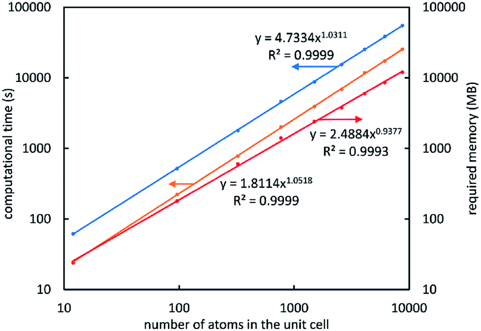 | ||
| Fig. 6 The computational time and memory requirements scale linearly with increasing number of atoms in the unit cell. This plot contains data for periodic ice crystal supercells. The blue line is the total DDEC6 analysis computational time. The orange line is the computational time for bond order computation. The red line is the total amount of random access memory (RAM) required to perform the entire DDEC6 analysis. | ||
4.4 Statistical analysis
Four different types of statistical analysis were used in this work. First, statistical analysis was used to quantify the failure modes of different bond index methods for different spin states and bond lengths of the oxygen molecule. Second, statistical analysis was used to fit parameter values in the comprehensive bond order equation. Third, statistical analysis was used to quantify the performance of the comprehensive bond order equation across diverse chemical systems. Fourth, statistical analysis was used to quantify the accuracy of computed material geometries.Statistical analysis used to quantify the failure modes of different bond index methods is now summarized. Three different failure modes were investigated: (1) failure of the bond index method to produce similar bond indices for similar electron density distribution inputs, (2) failure of the bond index method to produce a smooth curve of the bond index with increasing bond length, and (3) failure of the bond index method to converge to a solution. Mostly importantly, the conclusions drawn were robust to the choice of test system and threshold between success and failure. First, fundamental attributes of the bond index methods themselves rather than particular choice of test system determined which methods passed or failed each mode. Specifically, all bond index methods that were (were not) a functional of the electron and spin distributions passed (failed) the type 1 test set. Only the type 2A bond index methods (i.e., bond index is a functional of the electron and spin distributions) that used an exponentially decaying electron density tail for each atom passed the type 2 test set. Some of the bond index methods that required orbital localization (i.e., ANDP, Cioslowski, NBO, and NLMO) exhibited convergence failure (type 3 error) for at least one geometry.
Because the performance difference between passing and failing methods was huge, these findings were robust to the precise choice of threshold between success and failure. In other words, each method that failed did so in a spectacular and unambiguous manner. Specifically, each method failing the type 1 test set had at least one type 1 error ≥1.82. The type 1 error threshold was set to 0.3. Therefore, even increasing the type 1 error threshold by a factor of six would not have caused any methods failing the type 1 test set to pass it. For the stretched O2 molecule, the maximum type 1 error for methods passing the type 1 test set was 0.13. Therefore, more than an order of magnitude difference in performance separated those methods passing the type 1 test set from those failing it. With the type 1 error threshold set to 0.3, each failing method managed to fail profusely. Specifically, each failing method managed to fail more than 50% of the type 1 tests, even though only one failure would have been sufficient to classify the method as failing. Among the 13 different bond indices tested, only the DDEC6 bond order, DDEC6 contact exchange, DDEC6 overlap population, and the Laplacian bond index passed the type 1 test set. The Laplacian bond index failed 5 of 24 type 2 tests. Moreover, in all five of these failures, the type 2 error metric was ≤0.24. Even if the type 2 threshold between success and failure was made twice as generous (i.e., ≤1/4 or ≥4 for failure instead of ≤½ or ≥2), then the Laplacian bond index would still have failed 5 of 24 type 2 tests. Thus, overall conclusions about which bond index methods failed were insensitive to the precise threshold values separating success from failure.
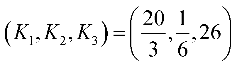
Statistical analysis used to fit parameter values in the comprehensive bond order equation is now summarized. The comprehensive bond order equation uses three parameter values: K1 = 20/3, K2 = 1/6, and K3 = 26. K1 affects the computed bond orders in all materials. K2 has a negligible effect when the contact exchange between two atoms is small (≪1) and a substantial effect when the contact exchange is large (≫1). K3 affects the computed bond orders only in materials having more than two atoms. Therefore, by careful choice of materials, I fitted the value of K1 first, then K2, and finally K3 rather than fitting all three parameter values simultaneously. In fitting the value of K1, I combined the results of Wheatley and Gopal's bond-order-to-overlap-population ratio correlation38 for small molecules with a new partition approximation of the dressed-exchange hole for diatomic molecules. The value of K2 was then fit via the observation that the bond-order-to-contact-exchange ratio for a quadruple bond approaches the upper bound of 2. The value of K3 was then optimized to give accurate SBOs for several materials whose target SBOs were determined using chemical arguments. Details of the derivation of the K1, K2, and K3 values are provided in Section S6 of ESI.†
Computational results across extremely diverse material types showed these K1, K2, and K3 values usually give bond orders and SBOs within ∼5% of optimality. Across the set of materials used for quantifying SBO transferability in Table 8, the SBOs (avg. ± st. dev.) were 0.98 ± 0.05 (H atoms), 3.19 ± 0.09 (B atoms), 3.96 ± 0.12 (C atoms), 3.43 ± 0.23 (N atoms), 2.22 ± 0.19 (O atoms), 1.06 ± 0.18 (F atoms), and 0.65 ± 0.17 (Na atoms). For H, B, and C, the standard deviations were ≤5% of the SBOs. For N, O, F, and Na, the standard deviations were greater than 5% of the SBOs, but this is due to physical reasons not computational error: (a) whether or not N atoms contain localized lone pairs (e.g., ∼3 versus ∼4 bonds per N atom), (b) Lewis acid–base lone-pair interactions, hydrogen-bonding, and extra π-bonding by O atoms, and (c) covalent versus ionic F and Na atoms. The SBOs for 55% of the 3d and 5d pure transition metal solids (Table 6) differed by ≤5% from the heuristic SBOs. For the period 1 and 2 homodiatomic molecules H2, Li2, N2, O2, and F2, the computed DDEC6 bond orders are all within 7% of the heuristic bond orders. For heavier homodiatomics, there are larger differences owing to physical effects such as partial exchange hole localization by semi-core electrons (e.g., Cs2) and bond strengthening effects (e.g., Cl2), which are described by the DDEC6 bond orders but not by the heuristic bond orders.
Increasing the accuracy of the computed bond orders and SBOs to within ∼1% of optimality is not feasible in practice at this time for the following reasons. First, approximations within the comprehensive bond order equation are not only due to the K1, K2, and K3 values, but also due to its overall functional form. Second, nearly exact electron and spin distributions are only available for small molecules and not for large dense materials with heavy atoms owing to the intrinsic difficulties associated with solving the multi-electronic equation exactly for large numbers of particles. Third, the charge and spin partitioning method employed (i.e., DDEC6) introduces approximations that affect the computed bond orders and SBOs. Taken together, it is infeasible to drive all cumulative errors in the computed bond orders and SBOs to better than ∼1% accuracy at this time, although errors better than ∼5% are typical as can be inferred from the comments in the previous paragraph.
Statistical analysis was used to quantify the performance of the comprehensive bond order equation across diverse chemical systems. SBO statistics (i.e., average, minimum, maximum, and standard deviation) were computed for each chemical element that appeared in at least five different materials, where diatomic molecules, stretched bonds, and transition states were excluded. These elements were H, B, C, N, O, F, and Na. Their SBO statistics are summarized in Table 8. Bond order statistics (i.e., average, minimum, and maximum) were computed for each bond type appearing in at least two different materials and having a total of at least five bonds of the given type. For transition states, bonds that formed or broke during the chemical reaction were not included in the bond type statistics. All bonds of the same type had the same nearest neighbors. For example, one C–C bond type had the first carbon atom bound to one C and one H atoms, and the second C atom bound to two C atoms. Thirteen such bond types were identified: six C–C bond types, three C–H bond types, two O–H bond types, one B–N bond type, and one C–F bond type. Their statistics are presented in Fig. 9. As discussed above, failure mode statistics were collected for the stretched O2 molecule, and heuristic versus DDEC6 SBOs were compared for the 3d and 5d transition metal solids.
The consistency of bond orders computed using coupled-cluster and DFT was quantified for 26 diatomic molecules. The DDEC6 bond order computed using the PBE exchange–correlation functional was −0.03 lower on average than the DDEC6 bond order computed using coupled-cluster, and the rms difference was 0.16. This shows reasonable consistency between the PBE and coupled-cluster results. For the stretched O2 molecule, the DDEC6 bond order computed using B3LYP was 0.02 higher on average than the DDEC6 bond order computed using coupled-cluster, and the rms difference was 0.03. This shows reasonable consistency between the B3LYP and coupled-cluster results.
Moreover, bond order statistics were computed for different SZ values comprising a spin multiplet. Because the different SZ values comprising a spin multiplet have energies that differ by only a small amount due to spin–orbit coupling, their optimized geometries and electron distributions are similar. Even though their spin distributions are dramatically different, their exchange–correlation energies are similar. Therefore, their computed bond orders should be close, but not necessarily identical. Six spin multiplets were studied at their equilibrium bond lengths: O2 quintet and the triplet states of O2, S2, Se2, Te2, and SiH2. The high SZ (i.e., SZ = S) state was computed using CCSD. The SZ = 0 state was computed using SAC-CI. The DDEC6 bond order for SZ = 0 was 0.01 higher on average than for SZ = S, and the rms difference was 0.04. CCSD (SZ = S) and SAC-CI (SZ = 0) based DDEC6 bond orders were also compared for the O2 quintet and triplet states at different bond lengths. The quintet state was studied at 188 (equilibrium), 200, 250, 300, 350, and 400 pm bond lengths. The triplet state was studied at 100, 120 (equilibrium), 150, 200, 250, and 300 pm bond lengths. The DDEC6 bond order for SZ = 0 was 0.03 lower on average than for SZ = S, and the rms difference was 0.04. These results show reasonable consistency in DDEC6 bond orders across SZ values comprising a spin multiplet.
In addition to the statistical analysis described above, accuracies of computed geometries for the diatomic molecules and pure transition metal solids were assessed through comparisons to previously published reference values. Except in a few cases where accurate experimental bond lengths were not readily available (i.e., [H2]+, Kr2, U2), all reference values are from experimental measurements. Reference bond lengths for the diatomic molecules were taken from Schaad and Hicks116 ([H2]+), Lim et al.117 (K2, Rb2, Cs2), Merritt et al.118 (Be2), Ogilvie and Wang119 (Kr2), Gagliardi and Roos78 (U2), and the CRC Handbook of Chemistry and Physics120 (all other diatomics). The coupled-cluster diatomic bond lengths were within 0.1% ± 1.4% (avg. ± st. dev.) of the reference values. The PBE-computed diatomic bond lengths were within 1.0% ± 2.6% (avg. ± st. dev.) of the reference values. This shows the computed diatomic bond lengths were highly accurate. The PBE-computed molar densities for the 3d and 5d pure transition metal solids were within −0.3% ± 6.1% (avg. ± st. dev.) of the experimental values listed in the CRC Handbook of Chemistry and Physics.120
5. Results and Discussion
5.1 Application to diatomic molecules
Table 4 summarizes bonding properties for 26 diatomic molecules chosen to represent a variety of chemical groups. At the equilibrium bond length, 0 < heuristic BO ≲ ½(bonding electrons − antibonding electrons). The right-hand inequality accounts for bond polarity in hetero-diatomics or electrostatic repulsion in [H2]+. For U2, a CASPT2 study78 showed that valence electrons occupy the following bonding orbitals: 7sσg (2 e), 6dπu (4 e), 6dσg (0.97 e), 6dδg (0.98 e) with the remaining valence electrons localized in nearly non-bonding 5f orbitals. Summing the reported78 bonding minus anti-bonding orbital populations and dividing by 2 gives 4.24, but neglecting the weakly overlapping 5f orbitals reduces the heuristic bond order to 4. Except for Kr2 (5.2% error), all coupled-cluster (CC) bond lengths were within 2.3% of experiments. The DFT-computed (PBE functional) bond lengths were also in reasonable agreement to experiments. Basis sets and other computational details are listed in Table 3.| 2S + 1 | B.D.E.a (kJ mol−1) | Heuristic B.O. | B.L.E. C.C. (%) | B.O. C.C. | B.O./C.E. ratio C.C. | B.O./O.P. ratio C.C. | B.L.E. PBE (%) | B.O. PBE | Δ(B.O.) PBE-C.C. | |
|---|---|---|---|---|---|---|---|---|---|---|
| a All bond dissociation energies except [H2]+ from ref. 120. | ||||||||||
| Hydrogen dimers | ||||||||||
| H2 | 1 | 436 | 1 | 0.1 | 0.94 | 1.68 | 1.69 | 1.2 | 0.93 | −0.009 |
| [H2]+ | 2 | ∼270 | ∼½ | 0.0 | 0.30 | 1.59 | 1.56 | 7.0 | 0.26 | −0.036 |
|
||||||||||
| Halogen dimers | ||||||||||
| F2 | 1 | 159 | ∼1 | −1.7 | 0.98 | 1.54 | 1.54 | 0.0 | 0.97 | −0.014 |
| Cl2 | 1 | 243 | ∼1 | −0.3 | 1.36 | 1.60 | 1.61 | 0.9 | 1.31 | −0.045 |
| Br2 | 1 | 194 | ∼1 | −0.4 | 1.26 | 1.58 | 1.60 | 1.1 | 1.19 | −0.078 |
| I2 | 1 | 152 | ∼1 | −1.1 | 1.26 | 1.59 | 1.60 | 0.7 | 1.18 | −0.078 |
|
||||||||||
| Halogen acids | ||||||||||
| HF | 1 | 570 | 0–1 | −0.4 | 0.80 | 1.52 | 1.50 | 1.4 | 0.82 | 0.025 |
| HCl | 1 | 431 | 0–1 | −0.4 | 0.99 | 1.62 | 1.60 | 1.1 | 0.97 | −0.016 |
| HBr | 1 | 366 | 0–1 | −0.3 | 0.99 | 1.62 | 1.61 | 1.1 | 0.97 | −0.021 |
|
||||||||||
| Alkali metal dimers | ||||||||||
| Li2 | 1 | 105 | ∼1 | 0.3 | 0.93 | 1.69 | 1.79 | 2.0 | 0.86 | −0.067 |
| Na2 | 1 | 75 | ∼1 | −0.6 | 0.78 | 1.64 | 1.82 | 0.2 | 0.71 | −0.073 |
| K2 | 1 | 57 | ∼1 | 1.0 | 0.70 | 1.62 | 1.89 | 1.5 | 0.64 | −0.067 |
| Rb2 | 1 | 49 | ∼1 | 1.6 | 0.66 | 1.60 | 1.90 | 2.1 | 0.60 | −0.058 |
| Cs2 | 1 | 44 | ∼1 | 1.2 | 0.62 | 1.60 | 1.87 | 2.1 | 0.56 | −0.054 |
|
||||||||||
| Weakly bound | ||||||||||
| Be2 | 1 | 59 | >0 | 2.3 | 0.65 | 1.57 | 1.64 | −3.1 | 0.70 | 0.054 |
| Kr2 | 1 | 5 | >0 | 5.2 | 0.03 | 1.42 | 1.43 | 8.0 | 0.03 | −0.001 |
|
||||||||||
| Group 16 dimers | ||||||||||
| O2 | 3 | 498 | ∼2 | −1.1 | 1.96 | 1.66 | 1.67 | 0.9 | 1.86 | −0.099 |
| S2 | 3 | 430 | ∼2 | −0.5 | 2.09 | 1.69 | 1.70 | 1.0 | 1.97 | −0.125 |
| Se2 | 3 | 331 | ∼2 | −0.9 | 1.87 | 1.66 | 1.66 | 1.2 | 1.69 | −0.178 |
| Te2 | 3 | 258 | ∼2 | −1.3 | 1.76 | 1.65 | 1.64 | 0.9 | 1.60 | −0.158 |
|
||||||||||
| Other p-block dimers | ||||||||||
| CO | 1 | 1077 | 2–3 | −0.5 | 2.58 | 1.75 | 1.78 | 0.6 | 2.51 | −0.068 |
| N2 | 1 | 945 | ∼3 | −0.5 | 2.92 | 1.79 | 1.82 | 0.4 | 2.84 | −0.074 |
| NO | 2 | 631 | ∼2½ | −0.9 | 2.40 | 1.72 | 1.74 | 0.5 | 2.32 | −0.077 |
| P2 | 1 | 489 | ∼3 | −0.7 | 2.55 | 1.76 | 1.76 | 0.5 | 2.43 | −0.129 |
|
||||||||||
| d-Block dimers | ||||||||||
| Cu2 | 1 | 182 | ∼1 | 2.1 | 1.05 | 1.58 | 1.55 | 0.0 | 1.11 | 0.061 |
|
||||||||||
| f-Block dimers | ||||||||||
| U2 | 7 | 222 | ∼4 | 1.3 | 3.79 | 1.82 | 1.95 | −7.0 | 4.48 | 0.693 |
The DDEC6 BOs followed the general trend of the heuristic BOs with the following caveats. First, the BO of [H2]+ is less than ½, because electrostatic repulsion between the partially charged H atoms gives a longer equilibrium bond length than for H2. Fig. 4 shows approximately exponential decay of the stretched H2 and [H2]+ bond orders with increasing bond length (see Section S9 of ESI† for a detailed breakdown of contributions to the optimized [H2]+ ion's bond order). Second, bond energies usually decrease when going down a chemical group, but the diatomic halogens have a maximum bond energy at Cl2 not F2. The DDEC6 BOs for diatomic halogens also exhibit a maximum at Cl2. The DDEC6 BOs for Cl2, Br2, and I2 are 1.26–1.36 while that for F2 is 0.98. Third, exchange between bonding and semi-core electrons can decrease delocalization of the bonding electrons leading to lower bond order. This effect is more pronounced when both bonding electrons and semi-core electrons are diffuse, such as occurs for elements to the left of each periodic row or for multiple-order bonds in heavy elements. In Table 4, this effect is evident for the heavy alkali metal dimers, for P2, and for Te2. This is related to the observation that period 2 elements form multiple-order bonds more easily in organic compounds than heavier elements.121
Table 4 includes several consistency checks. The DDEC6 BOs computed using the PBE functional were −0.03 lower on average than those computed using CC, with an rms difference of 0.16. This shows the method works well for both CC and DFT. For CC, the BO/CE ratios ranged from 1.42–1.82, which are within the feasible range of 1–2 (eqn (21)). The BO/OP ratios were similarly 1.43–1.95.
Owing to its multi-reference character,118 Be2 had to be modeled using SAC-CI instead of CCSD (using the def2qzvppd basis set, my CCSD and SAC-CI calculations yielded bond lengths of 4.56 (CCSD) and 2.51 (SAC-CI) Å compared to the experimental bond length118 of 2.45 Å). The molecular orbital diagram for Be2 predicts a “weak single bond” due to mixing of atomic s-pz orbitals to create a 1σg(2 e)1σu(2 e) molecular valence electron configuration, where “the 1σg orbital is bonding and the 1σu orbital is slightly anti-bonding”.6 Multi-reference configuration interaction calculations by Kalemos confirm the Be2 bond is sp hybridized.122 The DDEC6 BO of 0.65 for Be2 is indeed moderately less than one. Its dissociation energy (59 kJ mol−1) is similar to that for K2.
There is not an one-to-one correspondence between bond orders and bond energies. For example, the quadruply bonded U2 has much smaller dissociation energy than the singly bonded H2.
5.2 Application to pure transition metal solids
Pure transition metal solids contain partially filled and highly delocalized valence bands that make them good electrical conductors. Methods that study bonding by localizing orbitals have difficulties for metallic systems due to the inherent delocalization of conducting electrons. The bond orders introduced here are ideal for studying conducting metals, because no orbital localization is required. In fcc Cu, the DFT-computed QCT MBI between two adjacent Cu atoms has been reported as 0.26,123 which agrees with the DDEC6 bond order of 0.25 here.The 3d and 5d transition metal solids were studied as examples. Table 5 compares the experimental and computed magnetic alignment and atomic spin moments (ASMs) for each material. The experimental and calculated magnetic properties were in good agreement for all materials except Mn. Mn exhibits an extremely delicate magnetic ordering that is beyond the accuracy reach of existing DFT functionals.124 A range of values is reported for Mn, because the unit cell contains numerous inequivalent types of Mn sites.124
| Element | Low energy phase | Exp. ASM | Calc. ASM | Exp. magnetic alignment | Calc. magnetic alignment |
|---|---|---|---|---|---|
| a From ref. 125.b From ref. 124. A range of values is reported, because the different Mn atoms are not equivalent; the ASM magnitudes of individual Mn atoms in the structure fall at various points within this range.c From ref. 126. | |||||
| 3d transition metal elements | |||||
| Sc | hcp | 0 | 0.00 | None | Incipient |
| Ti | hcp | 0 | 0.00 | None | None |
| V | bcc | 0 | 0.00 | None | None |
| Cr | bcc | ∼0.4a | 1.05 | Anti-ferro | Anti-ferro |
| Mn | Alpha | 0–2.83b | 0–2.79b | Non-collinear | Incipient |
| Fe | bcc | 2.22c | 2.21 | Ferro | Ferro |
| Co | hcp | 1.71c | 1.61 | Ferro | Ferro |
| Ni | fcc | 0.61c | 0.64 | Ferro | Ferro |
| Cu | fcc | 0 | 0.00 | None | None |
| Zn | Distort. hcp | 0 | 0.00 | None | None |
|
|||||
| 5d transition metal elements | |||||
| Lu | hcp | 0 | 0 | None | None |
| Hf | hcp | 0 | 0 | None | None |
| Ta | bcc | 0 | 0 | None | None |
| W | bcc | 0 | 0 | None | None |
| Re | hcp | 0 | 0 | None | None |
| Os | hcp | 0 | 0 | None | None |
| Ir | fcc | 0 | 0 | None | None |
| Pt | fcc | 0 | 0 | None | None |
| Au | fcc | 0 | 0 | None | None |
| Hg | Rhom. | 0 | 0 | None | None |
The heuristic SBO = min(2 + min((NV − 2 − |ASM|), (12 − NV − |ASM|)), 6) has the following explanation. NV is the number of valence electrons, where a completely filled 4f shell is classified into core. First, two valence electrons are assumed to be available for s- or p-hybridized bonding, because in the aufbau principle there would nominally be predicted to remain 2 valence electrons outside the d-subshell. The remaining valence electrons are assumed to inhabit the d-subshell. Second, electrons that contribute to the ASM are assumed to be localized in d-orbitals that do not contribute to bonding. Because there are five d-orbitals that will fill via Hund's rule, the number of partially filled d-orbitals available for bonding is min((NV − 2), 10 − (NV − 2)) − |ASM|. Third, because the maximum number of close-packed nearest neighbors is 12 and each bond connects two atoms, the translational symmetry will normally accommodate up to 12/2 = 6 independent bonds to each atom. Consequently, the maximum natural SBO for an atom is 6, and SBOs >6 are exceptional.
Table 6 lists the experimental molar (mol L−1) and mass (g cm−3) densities and DFT-computed (PBE functional) molar densities. Except for Hg (−19% error), Mn (16% error), and Au (−5.5%), all computed molar densities were within ±5% of experiments. Across the 3d series, the density increases rapidly from Sc to Cr, changes slowly from Mn to Cu, and then decreases dramatically for Zn. The DDEC6 SBOs followed a trend similar to the densities. Due to complications mentioned above, a precise comparison of the DDEC6 and heuristic SBOs was not possible for Mn. For all other 3d elements, the heuristic and DDEC6 SBOs differed by ≤0.9.
| Element | Group (NV) | Low energy phase | Exp. molar dens. (mol L−1) | DFT molar dens. | Exp. mass dens. (g/cm3) | Heuristic SBO | DDEC6 SBO | SBO/SCE | SBO/SOP | Largest bond order |
|---|---|---|---|---|---|---|---|---|---|---|
| 3d transition metal elements | ||||||||||
| Sc | 3 | hcp | 66.5 | 67.2 | 2.99 | 3 | 2.77 | 1.16 | 1.24 | 0.24 |
| Ti | 4 | hcp | 94.1 | 95.8 | 4.506 | 4 | 3.52 | 1.14 | 1.18 | 0.30 |
| V | 5 | bcc | 117.8 | 123.3 | 6.0 | 5 | 4.10 | 1.13 | 1.15 | 0.39 |
| Cr | 6 | bcc | 137.5 | 141.1 | 7.15 | 4.95 | 4.36 | 1.12 | 1.13 | 0.41 |
| Mn | 7 | alpha | 132.9 | 153.6 | 7.3 | 3.21–6 | 3.82–4.70 | 1.08–1.14 | 1.08–1.14 | 0.72 |
| Fe | 8 | bcc | 140.9 | 146.2 | 7.87 | 3.79 | 3.97 | 1.12 | 1.12 | 0.37 |
| Co | 9 | hcp | 150.3 | 153.5 | 8.86 | 3.39 | 3.83 | 1.11 | 1.11 | 0.31 |
| Ni | 10 | fcc | 151.6 | 152.3 | 8.90 | 3.36 | 3.54 | 1.11 | 1.11 | 0.28 |
| Cu | 11 | fcc | 141.0 | 138.4 | 8.96 | 3 | 3.10 | 1.11 | 1.12 | 0.25 |
| Zn | 12 | Distort. hcp | 109.1 | 107.8 | 7.134 | 2 | 2.88 | 1.15 | 1.15 | 0.31 |
|
||||||||||
| 5d transition metal elements | ||||||||||
| Lu | 3 | hcp | 56.2 | 56.7 | 9.84 | 3 | 3.15 | 1.17 | 1.24 | 0.27 |
| Hf | 4 | hcp | 74.5 | 73.9 | 13.3 | 4 | 4.16 | 1.16 | 1.20 | 0.36 |
| Ta | 5 | bcc | 90.6 | 90.8 | 16.4 | 5 | 5.07 | 1.16 | 1.18 | 0.50 |
| W | 6 | bcc | 105.0 | 102.7 | 19.3 | 6 | 5.77 | 1.16 | 1.16 | 0.56 |
| Re | 7 | hcp | 111.7 | 111.1 | 20.8 | 6 | 5.88 | 1.14 | 1.14 | 0.48 |
| Os | 8 | hcp | 118.7 | 116.3 | 22.587 | 6 | 5.72 | 1.14 | 1.14 | 0.49 |
| Ir | 9 | fcc | 117.4 | 114.4 | 22.562 | 5 | 5.10 | 1.14 | 1.14 | 0.41 |
| Pt | 10 | fcc | 110.2 | 106.2 | 21.5 | 4 | 4.20 | 1.14 | 1.15 | 0.34 |
| Au | 11 | fcc | 98.0 | 92.6 | 19.3 | 3 | 3.41 | 1.14 | 1.14 | 0.28 |
| Hg | 12 | Rhom. | 67.5 | 54.9 | 13.5336 | 2 | 1.72 | 1.16 | 1.16 | 0.17 |
Across the 5d series, the density increases by more than a factor of two from Lu to Os, changes little from Os to Ir, and decreases by >40% from Ir to Hg. Likewise, the DDEC6 SBO increases, reaches a maximum, and then decreases. For each 5d element, the DDEC6 and heuristic SBOs differed by ≤0.41. The DDEC6 SBOs for W, Re, and Os are all ∼6. For a given SBO, one would expect a slight increase in density moving to the right within the 5d block, because the atomic mass increases and the atom slightly contracts. This explains why Os is slightly denser than W and Re. Upon going from Os to Ir, the heuristic and DDEC6 SBOs decrease along with the density. This explains why Os is the densest 5d element. Moreover, Os is the densest of all naturally occurring stable elements.120
The avg(DDEC6 SBO − heuristic SBO) = −0.048 (3d elements except Mn), 0.019 (5d elements), and −0.013 (3d & 5d elements except Mn). Thus, the overall average difference between DDEC6 and heuristic SBOs was tiny. The rms difference was 0.40. This correspondence between DDEC6 and heuristic SBOs ensures the computed DDEC6 bond orders are chemically accurate.
The last column in Table 6 lists the largest DDEC6 bond order for each material. This corresponded to the bond order between nearest neighbors. Because the bond order falls off approximately exponentially with increasing distance, the majority of the SBO is caused by nearby atoms with atoms far away contributing little.
It is not possible to obtain accurate bond orders using a constant bond-order-to-contact-exchange or bond-order-to-overlap-population ratio correlation. Specifically, the SBO/SCE ratio was 1.08–1.17 for the pure transition metal solids (Table 6) but 1.42–1.82 for the diatomics (Table 4). The DDEC6 bond-order-to-overlap-population ratios were similar to the bond-order-to-contact-exchange ratios.
5.3 Applications to spin multiplets
When no external magnetic field is applied, the various SZ values (e.g., SZ = −1, 0, 1) of a spin multiplet (e.g., triplet) differ in energy by only a small amount due to spin–orbit coupling.77 Here, the O2 triplet, O2 quintet, S2 triplet, Se2 triplet, Te2 triplet, and SiH2 triplet spin states were studied as examples. The ground state of silylene (SiH2) is a singlet,127 while the ground states of O2, S2, Se2, and Te2 are triplets.120 Here, the CCSD method was used to compute the electron and spin density distributions for SZ = S values: 0 for singlet, 1 for triplet, and 2 for quintet. The SAC-CI method was used to compute the electron and spin density distributions for SZ = 0. The spin density distributions of different SZ values of a spin multiplet must be dramatically different, because their integral is 2SZ. On the other hand, the electron density distributions of different SZ values of a spin multiplet are similar. This is illustrated by several density-derived descriptors listed in Table 7: optimized bond length, dipole moment magnitude, electronic spatial extent, and quadrupole moment eigenvalues. As shown in Table 7, these density-derived descriptors had similar values for the different SZ values comprising a spin multiplet. The small differences that occurred are in part due to the slightly different cutoffs of the CCSD and SAC-CI methods which produce an approximate rather than exact wavefunction.| S | SZ | Opt. bond length (Å) | μ | 〈r2〉 | Traceless quadrupole eigenvalues | |
|---|---|---|---|---|---|---|
| O2 | 1 | 1 | 1.19 | 0 | 22.7 | −0.18, 0.09, 0.09 |
| O2 | 1 | 0 | 1.20 | 0 | 22.6 | −0.20, 0.07, 0.12 |
| O2 | 2 | 2 | 1.88 | 0 | 23.3 | −0.39, −0.38, 0.77 |
| O2 | 2 | 0 | 1.88 | 0 | 23.5 | −0.43, −0.41, 0.84 |
| S2 | 1 | 1 | 1.88 | 0 | 56.4 | −0.47, −0.47, 0.94 |
| S2 | 1 | 0 | 1.88 | 0 | 56.4 | −0.48, −0.44, 0.92 |
| Se2 | 1 | 1 | 2.15 | 0 | 80.0 | −0.75, −0.75, 1.51 |
| Se2 | 1 | 0 | 2.15 | 0 | 80.1 | −0.74, −0.63, 1.37 |
| Te2 | 1 | 1 | 2.52 | 0 | 116.7 | −1.17, −1.17, 2.34 |
| Te2 | 1 | 0 | 2.52 | 0 | 117.2 | −1.13, −1.02, 2.15 |
| SiH2 | 1 | 1 | 1.48 | 0.02 | 34.8 | −0.82, 0.38, 0.44 |
| SiH2 | 1 | 0 | 1.48 | 0.04 | 34.8 | −0.83, 0.38, 0.45 |
The different SZ values comprising a spin multiplet have similar chemical reactivities. For example, molecular oxygen comprises about 20% of air. This molecular oxygen is primarily in the triplet spin state comprised of SZ = −1, 0, and +1 values. When burning an object such as wood in air, the different SZ values of the O2 triplet state react with essentially the same rates. In contrast, spin triplet and spin singlet O2 molecules have vastly different reactivities.
Because bond orders are intended to describe chemical properties, the similar chemical reactivities, energies, geometries, and density-derived descriptors of different SZ values comprising a spin multiplet imply their bond orders should also be similar. However, we will stop short of requiring their bond orders to be identical, because their energies, geometries, and density-derived properties are not exactly equal due to spin–orbit coupling. To produce similar bond orders for different SZ values comprising a spin multiplet, one might propose making the bond order a functional of the electron density distribution alone without any dependence on the spin density distribution. However, that would not be the most fundamental approach. Since electrons with different spins are considered distinguishable particles that are independently quantum blurred and do not exchange, the particle delocalization and hence bond order should depend on both the electron and spin density distributions. For proportional spin partitioning, propA(A)ρ() = ρA(A)(). Therefore, proportional spin partitioning would make the atomic exchange propensities simultaneously proportional to {ρA(A)} and {propA(A)}, which would make them similar for different SZ values of a spin multiplet. Similar bond orders for different SZ values comprising a spin multiplet thus requires the confluence of atomic exchange propensities in which {A(A)} are optimized to resemble {propA(A)}.
Computed DDEC6 bond orders are shown in Fig. 7. For the singlet state (e.g., SiH2 singlet), the CCSD and SAC-CI methods define the same mathematical problem and differ only in the numerical cutoffs employed. Accordingly, the CCSD and SAC-CI computed DDEC6 bond orders for the Si–H bond in singlet SiH2 are nearly identical. The triplet (O2, S2, Se2, Te2, SiH2) and quintet (O2) results show the DDEC6 bond orders are reasonably consistent across the various SZ values comprising a spin multiplet.
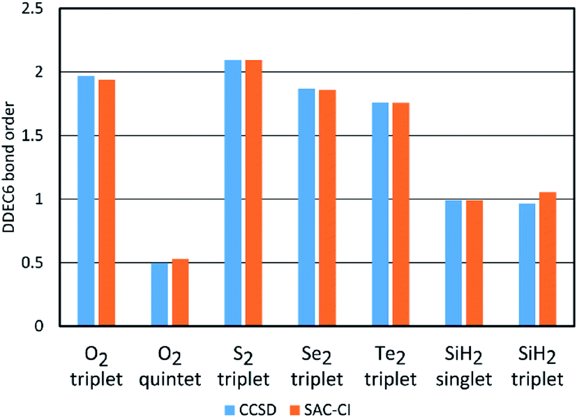 | ||
| Fig. 7 DDEC6 bond orders are reasonably consistent across the various SZ values comprising a spin multiplet. The CCSD results correspond to SZ = S, while the SAC-CI results correspond to SZ = 0. | ||
5.4 Application to non-collinear magnetism
Non-collinear magnetism occurs when the spin magnetization density direction,![[m with combining circumflex]](https://www.rsc.org/images/entities/i_char_006d_0302.gif) (), varies as a function of position in space. Computing accurate bond orders for non-collinear magnetism is challenging, because electrons in these systems cannot be classified as separately exchanging spin-up and spin-down populations. The comprehensive bond order equation is even accurate for systems having non-collinear magnetism. The Fe4O12N4C40H52 single molecule magnet is shown as an example in Fig. 8. DDEC6 NACs and ASMs for this material were previously reported in ref. 74. The non-collinear magnetism is shown by Fe ASM vectors (orange arrows) pointing in different directions. SBOs of ∼1 (H), ∼4 (C), ∼3.7 (N), and ∼2.5 (O) are in the typical range for organic and organometallic compounds. SBOs of 2–3 for O atoms are not unusual, because an isolated O atom has two unpaired valence electrons to share and can potentially participate in additional bonding via hydrogen bonds, Lewis acid–base lone pair interactions, or extra π-bonding. In this compound, the Fe atoms exhibited SBOs of ∼3. The individual computed bond orders were also reasonable, as shown by computed bond orders of 0.82–0.91 for C–H single bonds, the methanol C–O bond order of 1.18, and C–C bond orders of 1.15–1.53 in the aromatic C6 ring. These results show the DDEC6 bond order works well for non-collinear magnetism.
(), varies as a function of position in space. Computing accurate bond orders for non-collinear magnetism is challenging, because electrons in these systems cannot be classified as separately exchanging spin-up and spin-down populations. The comprehensive bond order equation is even accurate for systems having non-collinear magnetism. The Fe4O12N4C40H52 single molecule magnet is shown as an example in Fig. 8. DDEC6 NACs and ASMs for this material were previously reported in ref. 74. The non-collinear magnetism is shown by Fe ASM vectors (orange arrows) pointing in different directions. SBOs of ∼1 (H), ∼4 (C), ∼3.7 (N), and ∼2.5 (O) are in the typical range for organic and organometallic compounds. SBOs of 2–3 for O atoms are not unusual, because an isolated O atom has two unpaired valence electrons to share and can potentially participate in additional bonding via hydrogen bonds, Lewis acid–base lone pair interactions, or extra π-bonding. In this compound, the Fe atoms exhibited SBOs of ∼3. The individual computed bond orders were also reasonable, as shown by computed bond orders of 0.82–0.91 for C–H single bonds, the methanol C–O bond order of 1.18, and C–C bond orders of 1.15–1.53 in the aromatic C6 ring. These results show the DDEC6 bond order works well for non-collinear magnetism.
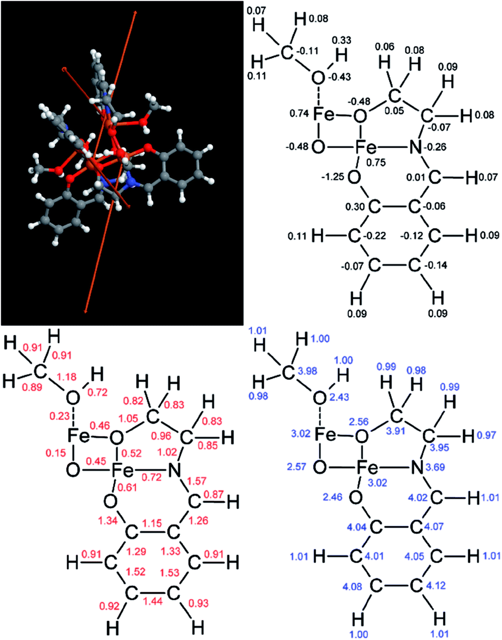 | ||
| Fig. 8 The Fe4O12N4C40H52 single molecule magnet (top left) contains a Fe4O4 distorted cuboid with Fe and O atoms on alternating corners attached to organic ligands. The non-collinear magnetism is shown by Fe ASM vectors (orange arrows) pointing in different directions. ASM vectors are negligible for the other atoms. The computed DDEC6 NACs (top right), bond orders (lower left), and SBOs (lower right) are shown for symmetry unique atoms. The full structure is formed by joining and overlapping four such units to form the Fe4O4 distorted cuboid bonded to four sets of methanol molecules and aromatic organic ligands. A methanol molecule is bound to each Fe atom via a Lewis acid-base interaction (dashed line) of bond order 0.23. | ||
5.5 Applications to other materials
DDEC6 bonding analysis gives excellent performance across a wide range of bonding types and materials. The DDEC6 bond orders and SBOs were tested and gave accurate results for the following bonding types: covalent, polar-covalent, ionic, aromatic, electron deficient multi-centered, dative (also called coordinate covalent bonding or Lewis acid–base interaction), metallic, dispersion, hypercoordinate, agostic, opportunistic, and hydrogen bonding. Stretched bonds, transition states, and ground state geometries were studied. A large variety of chemical structures were investigated: diatomics, biomolecules and other molecules, organometallic complexes, ions, collinear and non-collinear magnetic materials, sheets, polymers, spin multiplets, ionic solids, covalent solids (electrically insulating, conducting, and semi-conducting), porous and non-porous solids, Lewis adducts, catalysts, fullerenes, solid surfaces, metals, nanostructures, etc. The DDEC6 method is applicable to chemical elements 1 to 109.70As shown by numerous examples presented in this article, the valence electron configuration and the degree of coordinative saturation have primary roles in determining the SBO. Other structural details have secondary roles. Consider the Lu (hcp), Hf (hcp), Pt (fcc), and Au (fcc) crystal structures. Lu and Au have SBOs and nominal number of bonding electrons of ∼3, while Hf and Pt have SBOs and nominal number of bonding electrons of ∼4. Therefore, it is the valence electron configuration determining the number of bonding electrons not the crystal structure geometry that has the most influence on the SBO. Hypercoordinate systems can exhibit higher than typical SBOs. As shown in an example below, the S SBO for SF6 is 5.72. On the other hand, coordinatively unsaturated materials such as the CO molecule can exhibit lower than typical SBOs. For example, the C SBO for CO is only 2.58 compared to the typical C SBO of ∼4.
Table 8 reports SBO statistics for H, B, C, N, O, F, and Na atoms in the materials that were neither diatomics nor transition states. The H, B, C, and F SBOs were consistent with each of these elements sharing ∼1, ∼3, ∼4, and ∼1 bonding electrons per atom, respectively. Whether or not a N atom contained an electron lone pair (e.g., ∼3 versus ∼4 bonds per N atom) strongly affected its SBO. Lewis acid–base lone-pair interaction, hydrogen-bonding, or extra π-bonding by an O atom sometimes increased its SBO to ∼2.5. As expected, the Na atoms exhibited lower SBOs for the ionic materials than for the covalent materials.
| H | B | C | N | O | F | Na | |
|---|---|---|---|---|---|---|---|
| Avg. | 0.98 | 3.19 | 3.96 | 3.43 | 2.22 | 1.06 | 0.65 |
| St. dev. | 0.05 | 0.09 | 0.12 | 0.23 | 0.19 | 0.18 | 0.17 |
| Min. | 0.73 | 3.01 | 3.64 | 2.80 | 1.53 | 0.74 | 0.43 |
| Max. | 1.25 | 3.40 | 4.24 | 3.72 | 2.88 | 1.30 | 0.94 |
Fig. 9 reports statistics for bond types that occurred in at least two materials and at least five times in total. For transition states, bonds formed or broken during the chemical reaction were not included in the bond type statistics. The set of nearest neighbors defined each bond type. For example, one C–C bond type had the first carbon atom bound to one C and one H atoms, and the second C atom bound to two C atoms. Thirteen such bond types were identified: six C–C, three C–H, two O–H, one B–N, and one C–F. For each bond type, the DDEC6 bond orders had excellent transferability across different chemical structures.
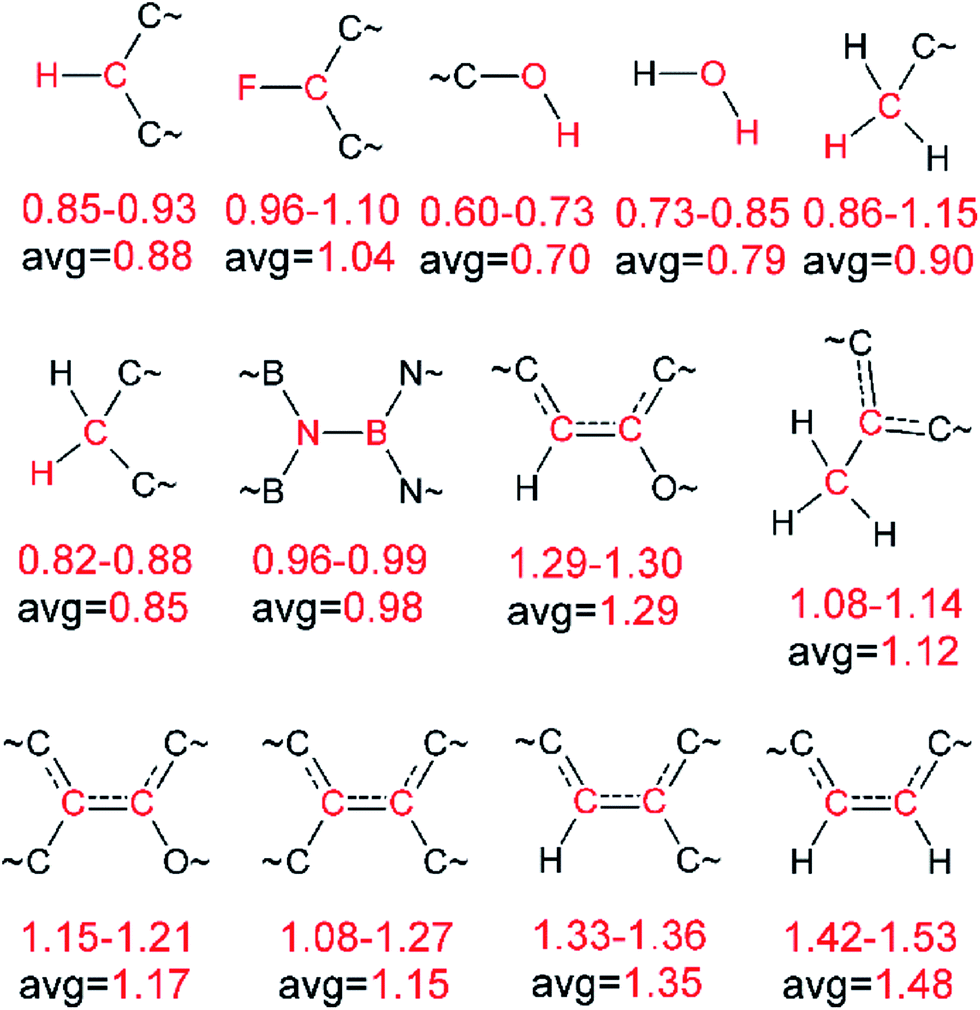 | ||
| Fig. 9 The range and average of DDEC6 bond orders for thirteen different bond types. The directly connected (red) and adjacent connected (black) atoms defined each bond type. A tilde (∼) indicates further bond connections to the remaining structure, but the specific form of these did not affect the bond type. Dashed lines indicate delocalized π-electrons. Each bond type displayed here occurred in at least five bonds distributed over at least two materials. DDEC6 bond orders for each bond type showed excellent transferability between different materials. | ||
The computed SBOs and bond orders are summarized in figures. Fig. 10 shows results for three nanostructured aromatic carbonaceous materials: graphene, graphite, and [Eu@C60]+. Fig. 11 summarizes results for five structures containing B–N bonds: H3N·BF3, B4N4, BN nanotube, BN sheet, and h-BN solid. Fig. 12 reports polyfluoroprene. Fig. 13 details diborane. Fig. 14 expresses results for three triatomics: [H–H–F] transition state, Na3 cluster, and ozone singlet. Fig. 15 displays the SF6 and [DbF6]− octahedral structures. Fig. 16 illustrates a synthetic analog of an enterotoxin produced by Escherichia coli bacterium. Fig. 17 depicts three hydrogen bonding structures: natrolite (a zeolite), the common ice crystal, and an ice surface. Fig. 18 illustrates seven simple solids: lithium, sodium, potassium, diamond, silicon, sodium fluoride, and table salt (sodium chloride). Fig. 19 depicts the Cu3BTC2 metal–organic framework exhibiting collinear anti-ferromagnetism. Fig. 20 reports two organometallic structures: (a) a chain initiation transition state for ethylene polymerization over a half-sandwich Ti catalyst ion pair, and (b) a half-sandwich Ti organometallic cation exhibiting opportunistic Ti–Br bonding.
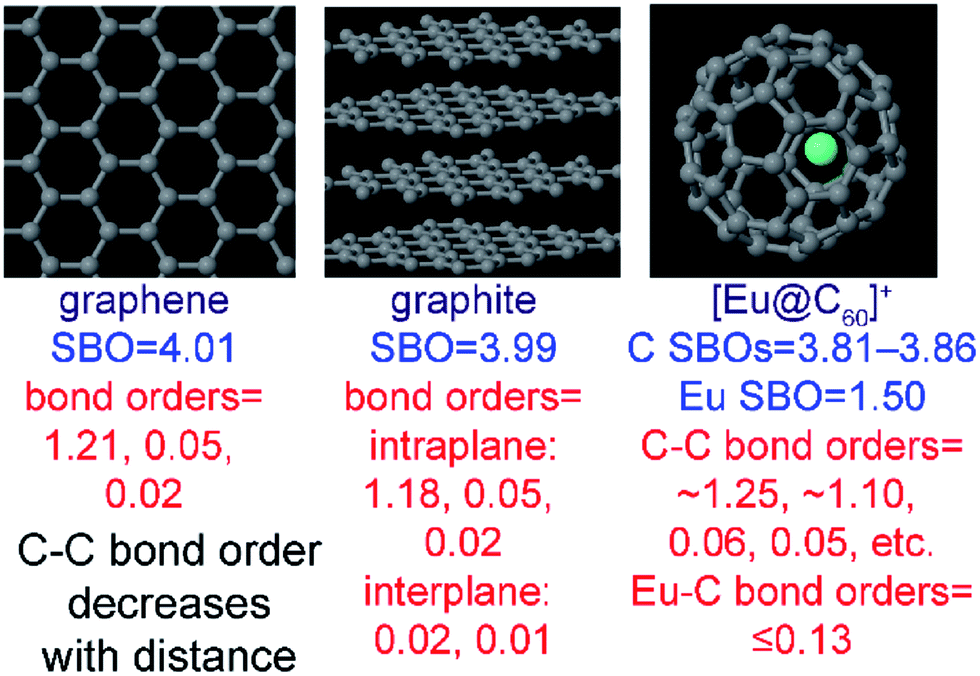 | ||
| Fig. 10 DDEC6 bonding analysis for three nanostructured materials with a high content of aromatic carbon atoms: graphene, graphite, and [Eu@C60]+. | ||
Fig. 10 illustrates three nanostructured materials with a high content of aromatic carbon atoms: graphene, graphite, and [Eu@C60]+. The DDEC6 SBO of each carbon atom is ∼4 in all three materials. This agrees with the fact that each carbon atom has four valence electrons to share in covalent bonding. Since each carbon atom in these structures is covalently bound to three adjacent carbon atoms, the bond order between adjacent carbon atoms would be expected to be 4/3 = 1.33 if all four valence electrons were shared only between nearest neighbors. However, there is a small amount of electron sharing between non-nearest neighbors, which reduces the C–C bond orders between nearest neighbors to slightly less than 4/3. For graphite, the DDEC6 bond order of 1.18 between adjacent C atoms is similar to the previously reported QCT MBI of 1.20.123 Graphene and graphite contain only one type of nearest neighbor bond. Weak London dispersion forces hold graphite layers on top of each other, and the DDEC6 bond orders between carbon atoms in different graphitic planes is ≤0.02. The C60 fullerene (aka buckyball) has the shape of a truncated icosahedron containing twenty hexagons and twelve pentagons. Each carbon atom in C60 has one bond of ∼1.25 order for a shared hexagon–hexagon edge and two bonds of ∼1.10 order for shared pentagon–hexagon edges. In the [Eu@C60]+ endohedral fullerene, all of the Eu–C bond orders are ≤0.13. These examples demonstrate the comprehensive bond order equation accurately applies to nanostructured carbonaceous materials.
Fig. 11 shows computed DDEC6 SBOs (blue) and selected bond orders (red) for five structures containing B–N bonds. H3N·BF3 is a Lewis acid–base adduct having a B–N bond order of 0.54. H3N is the Lewis base that provides a shared electron pair to the Lewis adduct. The other four structures demonstrate the accuracy of the comprehensive bond order equation across systems having different numbers of periodic dimensions: no periodicity (B4N4), 1D periodicity (BN nanotube), 2D periodicity (BN sheet), and 3D periodicity (h-BN solid). In all five structures, the B–N bond is polar-covalent with B NACs of 0.73–0.97, N NACs of −0.83 to −0.73, B SBOs of 3.01–3.32, and N SBOs of 2.81–3.43. The hexagonally bonded BN nanotube, sheet, and solid have remarkably similar (i.e., transferable) bond orders and SBOs. In h-BN solid, the interlayer B–N bond order is 0.02, which indicates noncovalent interactions play an important role in the interlayer binding. Bonding in these hexagonal BN structures contrasts with graphene and graphite. In graphene and graphite, each C atom shares four bonding electrons and has bond orders greater than one with its three nearest neighbors. In the hexagonal BN structures, each B and N atom has single order bonds to each of its three nearest neighbors.
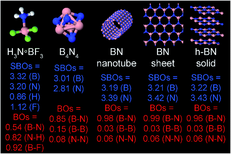 | ||
| Fig. 11 DDEC6 bonding analysis for five structures containing B–N bonds: H3N·BF3, B4N4 molecule, BN nanotube, BN sheet, and h-BN solid. | ||
Fig. 12 illustrates DDEC6 bonding analysis for polyfluoroprene. The C–C π-bond has a DDEC6 bond order of 1.64. The C–H, C–F, and other C–C bonds in the structure are approximately single bonds. The SBOs of ∼1 for H and ∼4 for C are consistent with the observation that each H (C) atom has one (four) electrons to covalently share. The SBO of F is greater than one (i.e., 1.30), because some of the F lone pairs exhibit a small overlap with nearby atoms.
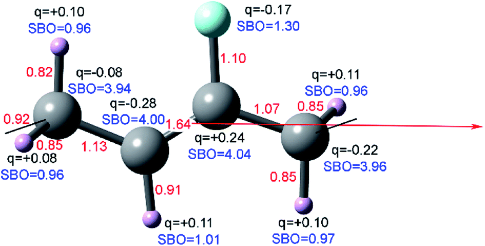 | ||
| Fig. 12 Computed DDEC6 bond orders (red), SBOs (blue), and NACs (black) for polyfluoroprene. This is an example of an organic polymer with one-dimensional periodic boundary conditions. The periodic lattice vector is illustrated by the red arrow. | ||
The diborane (i.e., B2H6) molecule is an example of an electron deficient molecule with multi-centered bonding. Fig. 13 summarizes DDEC6 analysis for diborane. The net atomic charges close to zero indicate nearly perfect covalent sharing of electrons among the atoms. The bond orders of 0.95 indicate single bonds between boron and the outer H atoms. The B–B bond and each bridging H–B bond are less than single order. The SBOs of ∼1 (∼3) for each H (B) atom are consistent with the observation that each H (B) atom has one (three) electrons to covalently share. The multi-centered bonding in diborane has been previously studied using a wide variety of other bond indices.15,17,22,25,38,52,128–131
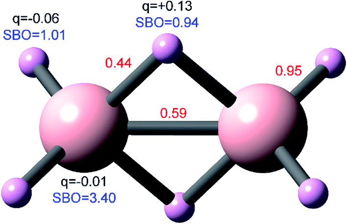 | ||
| Fig. 13 Computed DDEC6 bond orders (red), SBOs (blue), and NACs (black) for diborane. | ||
Fig. 14 summarizes DDEC6 analysis results for three triatomic systems: [H–H–F] transition state, Na3 cluster, and the ozone spin singlet. On the left is the transition state structure for the chemical reaction H2 + F ↔ H + HF. The computed results show the unpaired electron resides mainly on the F atom and the H–H bond is of higher order than the H–F bond in this transition state. The SBO of the middle H atom is 1.11. Because the SBO of the middle H atom is also approximately one in the reactant (i.e., H2 molecule) and product (i.e., HF molecule) states, this demonstrates an approximate (but not exact) conservation of total bond order along the reaction path. In the middle is shown the Na3 cluster. Because of the Jahn–Teller effect,132 this molecule forms an isosceles rather than an equilateral triangle. This triangle has two longer sides of bond order 0.22 and one shorter side of bond order 0.56. The computed results show the unpaired electron resides mainly on the Na atom that is farther from the other two Na atoms. On the right is shown the ozone singlet, which has significant multi-reference character. The bond order between the inner and outer oxygen atoms is 1.44. The bond order between the two outer oxygen atoms is 0.09. These three triatomic systems demonstrate the diversity of exchange–correlation methods that can be used to generate electron and spin density information used in DDEC6 analysis. The HF transition state was computed using a coupled-cluster method (i.e., CCSD). The Na3 cluster was computed using a dispersion-corrected density functional approximation (i.e., PBE+D3). The ozone singlet was computed using the complete active space self-consistent field (CAS-SCF) method, which is appropriate for studying multi-reference systems.
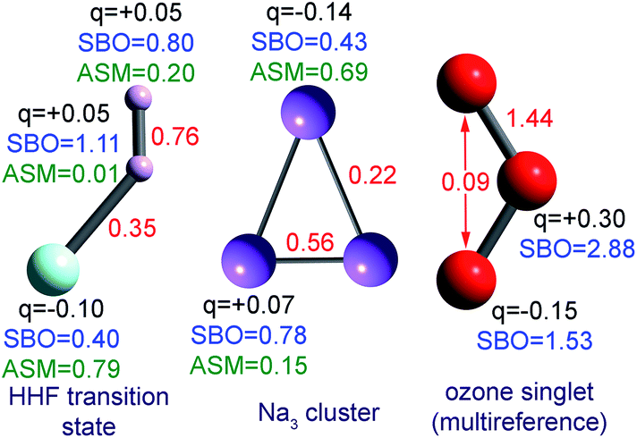 | ||
| Fig. 14 Computed DDEC6 bond orders (red), SBOs (blue), NACs (black), and ASMs (green) for three triatomic species. For the ozone singlet, the ASMs (not shown) are zero. | ||
Fig. 15 summarizes DDEC6 analysis for two hexafluorides: SF6 and [DbF6]−. SF6 is remarkably inert, has an estimated atmospheric lifetime of approximately 800–3200 years, and is one of the most potent greenhouse gases.133,134 It is used as an insulating dielectric in high voltage equipment,135,136 as a gas tracer,134,137,138 and in various specialized medical applications.139,140 The hypercoordinate nature of SF6 has been intensely debated.13,79,141–145 The computed DDEC6 NACs, S–F bond order of 0.95, and S SBO of 5.72 show SF6 contains six single-order S–F bonds rather than four multi-centered bonds. This result confirms that SF6 transcends the heuristic Lewis octet rule that predicts four rather than six shared electron pairs around the central sulfur atom. Dubnium is an artificially produced transactinide element with atomic number 105.120 The most stable dubnium isotope known to date has a half-life of approximately one day.120 Because of this short half-life, the chemistry of dubnium is not yet adequately explored.146 Shown here is a computed dubnium hexafluoride anion constrained to octahedral symmetry, but it is not yet known whether such a species actually exists in aqueous solutions.146 The Db–F bond length (2.00 Å) is longer than the S–F bond length (1.58 Å). The Db–F bond order (0.75) is also lower than the S–F bond order (0.95). Because Db is less electronegative than S, the F atoms have a more negative NAC in [DbF6]− than in SF6.
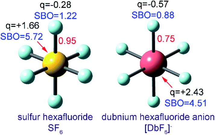 | ||
| Fig. 15 Computed DDEC6 bond orders (red), SBOs (blue), and NACs (black) for two hexafluorides. | ||
Bond orders help us understand the chemical structures of biomolecules. Fig. 16 illustrates a biomolecule (Protein Data Bank identifier 1ETM) that is a synthetic analog of an enterotoxin produced by Escherichia coli bacterium.80 1ETM is comprised of residues of the amino acids alanine, asparagine, cysteine, glutamic acid, glycine, leucine, proline, and a special modified protein residue. This structure contains three disulfide linkages with computed DDEC6 bond orders of 1.31–1.36 for S–S bonds and 1.02–1.06 for C–S bonds. Two carboxylic acid groups are present, and these have bond orders of 1.70–1.88 (C![[double bond, length as m-dash]](https://www.rsc.org/images/entities/char_e001.gif) O), 1.24–1.28 (C–OH), and 0.60–0.70 (O–H). The SBOs for each element were 0.73–1.25 (H), 3.83–4.24 (C), 3.39–3.72 (N), 2.03–2.28 (O), and 2.66–2.87 (S). The SBOs for H and C were consistent with covalent sharing of one and four valence electrons, respectively. The N and O SBOs were in typical range for organic compounds. Thus, the DDEC6 method is well-suited for studying biomolecules.
O), 1.24–1.28 (C–OH), and 0.60–0.70 (O–H). The SBOs for each element were 0.73–1.25 (H), 3.83–4.24 (C), 3.39–3.72 (N), 2.03–2.28 (O), and 2.66–2.87 (S). The SBOs for H and C were consistent with covalent sharing of one and four valence electrons, respectively. The N and O SBOs were in typical range for organic compounds. Thus, the DDEC6 method is well-suited for studying biomolecules.
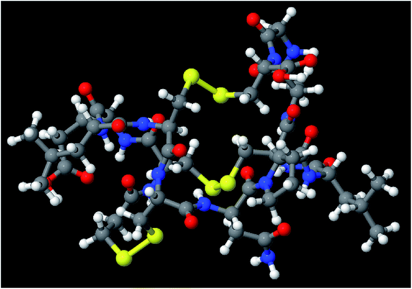 | ||
| Fig. 16 The 1ETM (Protein Data Bank identifier) biomolecule is a synthetic analog of an enterotoxin produced by Escherichia coli bacterium. Atoms are colored by element: H (white), C (gray), N (blue), O (red), S (yellow). This biomolecule is comprised of residues of the amino acids alanine, asparagine, cysteine, glutamic acid, glycine, leucine, proline, and a special modified protein residue. This structure contains three disulfide linkages. | ||
The DDEC6 method is well-suited for studying materials containing hydrogen bonds. Fig. 17 illustrates three materials containing hydrogen bonds: natrolite, ice crystal, and an ice solid surface. According to the IUPAC, “The hydrogen bond is an attractive interaction between a hydrogen atom from a molecule or a molecular fragment X–H in which X is more electronegative than H, and an atom or a group of atoms in the same or a different molecule, in which there is evidence of bond formation”.147 The hydrogen bond orders in these three materials were 0.07–0.13. The H NACs were 0.40–0.44. These results show the hydrogen bond contains a significant electrostatic character and a small covalent character.
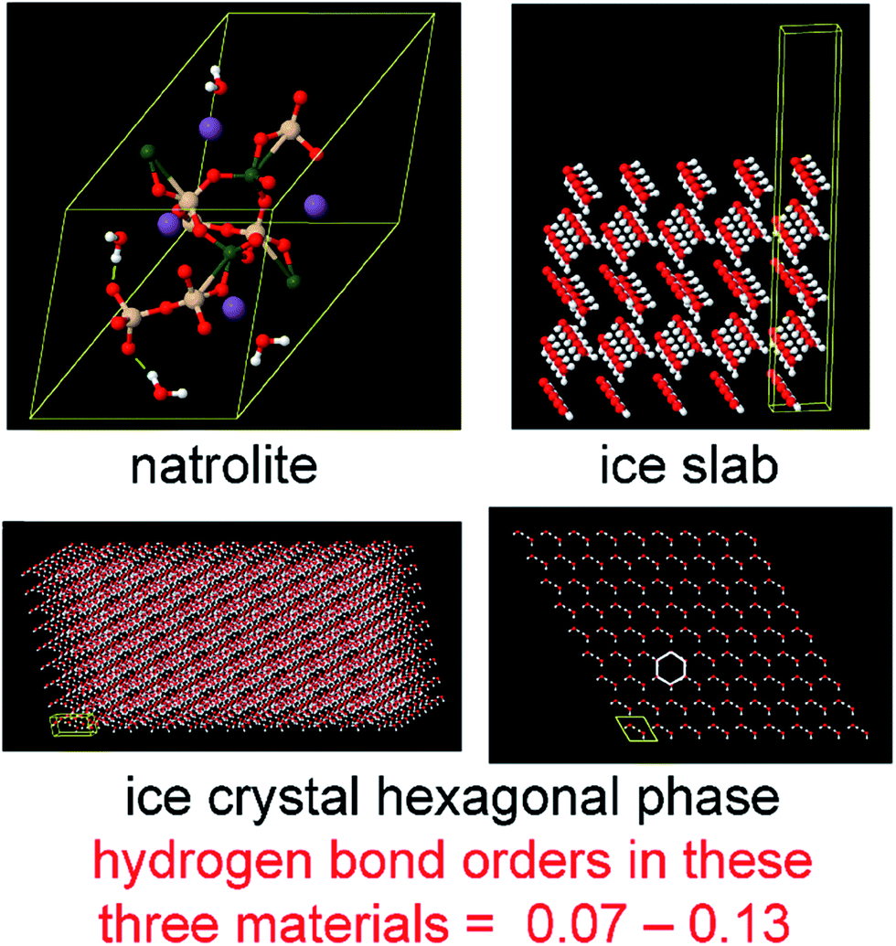 | ||
| Fig. 17 Three materials containing hydrogen bonds. In the structures shown above, the yellow lines mark the unit cell boundaries. Atoms are colored by element: H (white), O (red), Na (medium purple), Al (dark olive green), Si (desert sand). As shown in the top left, natrolite is a zeolite containing four water molecules per unit cell. As illustrated by the green lines, the hydrogen atoms from each water molecule hydrogen bond to the neighboring oxygen atoms bound to silicon. An ice slab is shown on the top right. Slabs are important test systems, because they contain both surface and buried atoms. The bottom left shows a large supercell of ice crystal hexagonal phase containing 8748 atoms. The bottom right shows an end view of the same structure with a hexagonal channel outlined in white. This hexagonal ice phase is the most common and makes up snowflakes and ice cubes. | ||
Fig. 18 shows DDEC6 bond orders and SBOs for seven simple solids. These include metallic covalent (Li, Na, K), insulating covalent (diamond), semi-conducting covalent (Si), and ionic (NaF, NaCl) solids. In the covalent solids, the SBOs of Li, Na, and K are ∼1, which is consistent with each of these elements having one valence electron to share in covalent bonding. In contrast, the previously reported QCT summed MBI of 1.60 for bcc Na overestimates the number of bonding electrons.123 The SBOs of C and Si are ∼4, which is consistent with each of these elements having four valence electrons to share in covalent bonding. The nearest neighbor C–C and Si–Si bond orders are slightly less than one in diamond and Si, because some electrons are shared between non-nearest neighbors. In the ionic solids NaF and NaCl, the SBOs of Na, F, and Cl are between 0 and 1, which reflects weak electron exchange between overlapping cations and anions. In these ionic solids, the F and Cl anions are more diffuse and have larger SBOs than the Na cations. DDEC6 bond orders for near neighbors in NaCl and diamond solids were 0.09 (Na–Cl), 0.03 (Cl–Cl), and 0.77 (C–C). For comparison, previously reported QCT MBI for NaCl and diamond solids were 0.07 (Na–Cl), 0.05 (Cl–Cl), and 0.91 (C–C).123
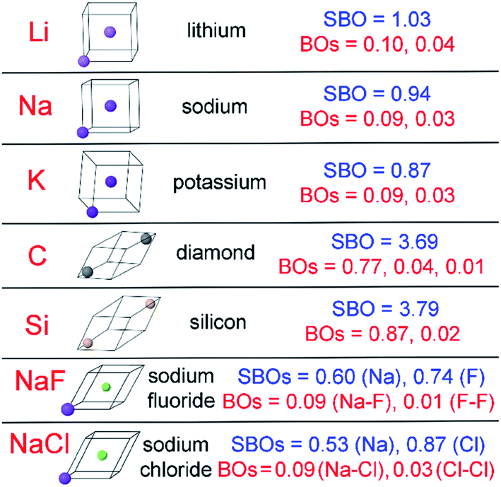 | ||
| Fig. 18 Computed DDEC6 SBOs and bond orders for seven simple solids. | ||
Fig. 19 summarizes DDEC6 analysis results for the Cu3BTC2 metal–organic framework (MOF). The 3-dimensional nanopore network is formed by connecting each Cu atom to four benzene-1,3,5-tricarboxylate (BTC) units and each BTC unit to six Cu atoms. Experiments by Zhang et al. showed there is anti-ferromagnetism between Cu atoms in each dimer.148 The DFT-computed magnetic structure is also collinear anti-ferromagnetism with each Cu dimer having one DDEC6 Cu ASM = +0.64 and one Cu ASM = −0.64. A small amount of electron spin (ASM = ±0.06) spills onto each O atom, while the C and H atoms are non-magnetic. The Cu (NAC = 0.83) and carboxylic C (NAC = 0.59) are positively charged, while the carboxylic O (NAC = −0.52) is negatively charged. As expected, C and H SBOs are ∼4 and ∼1, respectively. The O and Cu atoms have SBOs slightly greater than 2. The C–O bond order of the carboxylate group is near the ideal value of ∼1½, while the Cu–O bond order is ∼½. The Cu–Cu bond order (0.18) is weak.
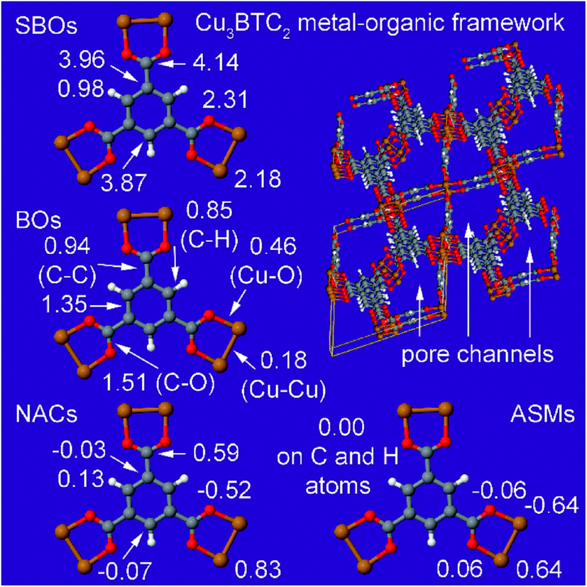 | ||
| Fig. 19 Computed DDEC6 SBOs, bond orders, NACs, and ASMs for the Cu3BTC2 metal–organic framework. Yellow lines mark the unit cell boundaries. Atoms are colored by element: H (white), C (gray), O (red), and Cu (copper). The illustrated SBOs, BOs, NACs, and ASMs are for the fully periodic crystal structure. | ||
Fig. 20 shows computed DDEC6 SBOs and bond orders (BO) for two half-sandwich Ti organometallic complexes. The top panel shows an ethylene polymerization backside chain initiation transition state having the structure [(C5Me5)Ti(OC6H2-2,6-Me2-4-Br)(CH3)(C2H4)]+ [MeB(C6F5)3]−. In this transition state, the ethylene CC bond is partially weakened (BO = 1.59) and bonds start to form between the incoming ethylene monomer and the Me initiating group (BO = 0.22) and Ti (BO = 0.31). There is also an agostic Ti–H(α-C) bond order = 0.07. The bottom panel shows a [(C5Me5)Ti(OC6H4-2-Br)(CH3)]+ cation exhibiting an opportunistic halogen bond between the Br and Ti atoms that dramatically impacts catalyst reactivity.89 The computed Ti–Br opportunistic BO is 0.24 and leads to this Br having a SBO of 1.47 instead of ∼1. The C–O aryloxide BO is 1.20 (top panel) and 1.33 (bottom panel). This is consistent with a study showing π-bonding along the Ti–O–C aryloxide linkage.149 This π-bonding produces a nearly linear Ti–O–C angle149 (top panel) but is bent by the Ti–Br opportunistic coordination (bottom panel). Each of the five carbon atoms in the pentagon is bonded to Ti with a BO = 0.13–0.21 to give a total Ti–C5 bond order of ∼1.
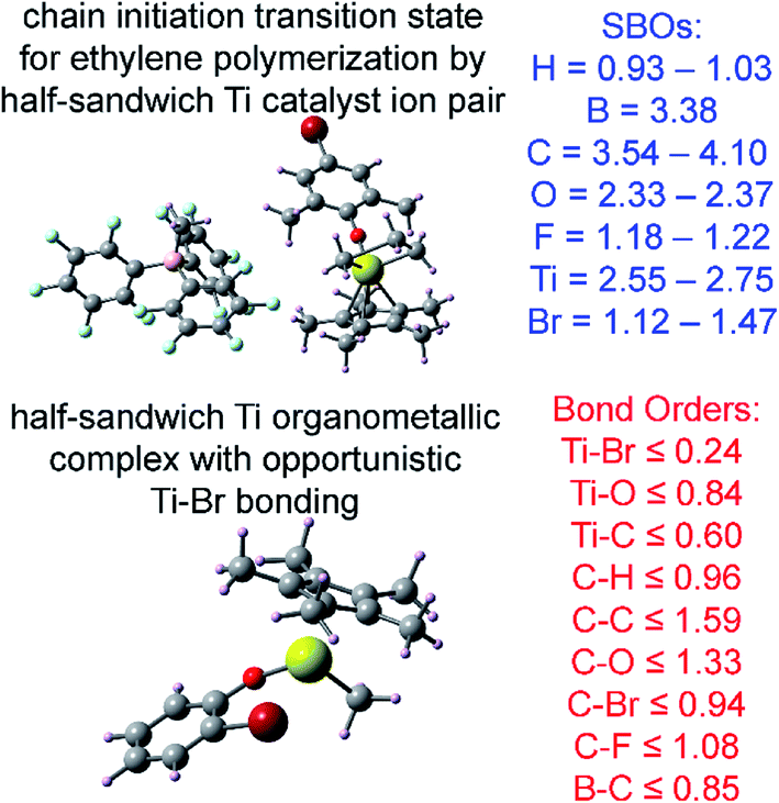 | ||
| Fig. 20 Computed DDEC6 SBOs and bond orders for two half-sandwich Ti organometallic complexes. | ||
6. Conclusions
The chemical sciences have lacked a suitable definition for bond order. The adaptive natural density partitioning (ANDP), Cioslowski, first-order delocalization index (FODI), Mayer, natural bond order (NBO), and natural localized molecular orbital (NLMO) bond indices do not provide approximately consistent results across different quantum chemistry methods (e.g., DFT, coupled-cluster, configuration interaction) and different SZ values of a spin multiplet, because these bond indices specifically depend on the natural orbitals and their occupancies which vary according to the quantum chemistry method. While the contact exchange, Laplacian bond index, and density-derived atom–atom overlap populations computed as functionals of the electron and spin magnetization density distributions do provide approximately consistent results across different quantum chemistry methods and different SZ values of a spin multiplet, those results are not constantly proportional to bond orders. The second-order delocalization index (SODI) that partitions the exchange–correlation hole into atom–atom pairwise components should yield similar results across different correlated quantum chemistry methods and SZ values of a spin multiplet. However, SODI measures something distinct from bond order.17 In some cases, SODI values approximately track bond orders, but in other cases SODI values and bond orders are quite different.17,22,27 Finally, the notion of bond orders as one-half the difference between bonding orbital and anti-bonding orbital occupancies does not work for stretched bonds.In this article, I presented a new theory of bond order that provides accurate results across an extremely diverse range of materials and bonding types. I showed bond order can be derived using a dressed exchange hole partitioned among atoms as a functional of the electron and spin magnetization density distributions. This dressed exchange hole differs from the pure exchange hole in ways that allow bond order to be more accurately computed. Also, I introduced the confluence of atomic exchange propensities that facilitates accurate and robust bond order computation. After introducing the contact exchange, I derived lower (1×) and upper (2×) bounds on the bond-order-to-contact-exchange ratio. Then, I derived a comprehensive equation (eqn (22)) for computing bond orders from first-principles quantum chemistry calculations. Terms in this equation are briefly explained in Fig. 3. This equation is unique and fundamental, because it has the simplest form that accurately captures the primary bond order effects. It applies to non-magnetic materials, collinear magnetism, and non-collinear magnetism. It depends only on the electron and spin magnetization density distributions. This makes bond orders easy to compute using widely available data conveniently output from nearly all quantum chemistry software packages. As shown in Fig. 6, its required computational time and memory scale linearly with increasing number of atoms in the unit cell, which even makes it applicable to systems containing many thousands of atoms.
DDEC6 atomic population analysis is optimal for computing the atomic electron and spin magnetization density distributions, {avgA(rA)} = {ρavgA(rA),avgA(rA)}, used as inputs to this comprehensive bond order equation. DDEC6 analysis satisfies the confluence of atomic exchange propensities. DDEC6 analysis also has exponentially decaying atom tails resembling real atoms, converges rapidly and robustly to a unique solution, has constraints to prevent buried atoms from becoming too diffuse or too contracted, provides a physically correct description of electron and spin transfer between atoms in materials, is computationally efficient, and applies to an extremely wide range of material types.70,74
Some students find learning chemistry difficult, because they have trouble memorizing which heuristic electron assignment model to apply to each chemical type. This comprehensive bond order could help students who prefer a more unified and computational approach to learning chemistry. Therefore, it may be appropriate to introduce into chemistry, materials science, and biochemistry textbooks for advanced college students adept at computer calculations.
This method can help anyone who wants to quantify bond orders in materials. It will be valuable to scientists and engineers by providing clearly defined bond order that can be computed and compared across various material types. For example, this will enable the study and comparison of bond orders for diatomic molecules reacting on a conducting metal surface, where bond orders must simultaneously account for localized bonding within diatomic molecules as well as highly delocalized bonding in the conducting metal. It can make bond order comparisons more unified across the many research articles published in chemical science journals.
Tests using an extremely diverse set of materials including at least one element from each chemical group (i.e., groups 1 to 18, lanthanides, actinides, and transactinides) and period (i.e., periodic rows 1 to 7) showed this method yields accurate results across most of the diversity of materials and bonding types encountered throughout the chemical sciences. It performed well for small molecules, a biomolecule, a polymer, porous solids, nonporous solids (electrically conducting, semiconducting, and insulating), a solid surface, a hypercoordinate molecule, an electron deficient molecule, hydrogen bound systems, transition states, Lewis acid–base complexes, aromatic compounds, magnetic systems, ionic materials, dispersion bound systems, nanostructures (clusters, tubes, sheets, etc.), and other materials. Notably, this method worked extremely well both for systems with localized bonding electrons (e.g., diatomic molecules) as well as for materials with highly delocalized bonding electrons (e.g., metallic solids). It worked well for stretched and compressed bond lengths.
Already, this new bond order improves our understanding of bonding in the 3d and 5d transition metal solids, Be2, and [H2]+. The molar and mass densities of pure 5d transition metal solids are correlated to their SBOs. The densest element osmium has SBO = ∼6. Be2 has a slightly lower than single-order covalent bond. [H2]+ has a bond order of ∼0.3 near its equilibrium length, and this decreases smoothly as the bond is stretched.
The computed DDEC6 bond orders were consistent across different quantum chemistry methods (e.g., DFT, coupled-cluster, configuration interaction) and different SZ values of a spin multiplet. Both the individual bond orders and the sum of bond orders for each atom in a material were shown to be reliably accurate across various bonding types: metallic, covalent, polar-covalent, ionic, aromatic, dative, hypercoordinate, electron deficient multi-centered, agostic, and hydrogen bonding. The DDEC6 bond orders also had good transferability between similarly bonded materials. Therefore, this new definition of bond order should be widely adopted by the chemical sciences.
Conflicts of interest
There are no conflicts to declare.Acknowledgements
NSF CAREER award DMR-1555376 provided financial support. The Extreme Science and Engineering Discovery Environment150 (NSF ACI-1053575) project TG-CTS100027 provided computational time on the Comet cluster at the San Diego Supercomputing Center and the Stampede cluster at the Texas Advanced Computing Center. The DDEC6 method is implemented in the CHARGEMOL software.115 I thank the reviewers for useful comments and for suggesting some of the references.References
- L. G. Wade and J. W. Simek, Organic Chemistry, Pearson, Glenview, IL, 9th edn, 2017 Search PubMed.
- Jmol: an open-source Java viewer for chemical structures in 3D, http://www.jmol.org/, accessed August 2017.
- R. M. Hanson, J. Appl. Crystallogr., 2010, 43, 1250–1260 CAS.
- D. D. Ridley, J. Chem. Inf. Comput. Sci., 2000, 40, 1077–1084 CrossRef CAS PubMed.
- D. D. Ridley, J. Chem. Educ., 2001, 78, 559–560 CrossRef CAS.
- R. L. Dekock and H. B. Gray, Chemical Structure and Bonding, University Science Books, Sausalito, CA, 2nd edn, 1989 Search PubMed.
- I. Sumar, R. Cook, P. W. Ayers and C. F. Matta, Phys. Scr., 2016, 91, 013001 CrossRef.
- C. F. Matta, I. Sumar, R. Cook and P. W. Ayers, in Applications of Topological Methods in Molecular Chemistry, ed. R. Chauvin, C. Lepetit, B. Silvi and E. Alikhani, Springer International Publishing, Cham, Switzerland, 2016, ch. 3, pp. 53–88 Search PubMed.
- M. Deshpande, M. Kuramochi, N. Wale and G. Karypis, IEEE Transactions on Knowledge and Data Engineering, 2005, 17, 1036–1050 CrossRef.
- C. Borgelt and M. R. Berthold, Mining Molecular Fragments: Finding Relevant Substructures of Molecules, in IEEE International Conference on Data Mining, IEEE, Maebashi City, Japan, 2002, pp. 51–58 Search PubMed.
- G. Frenking and A. Krapp, J. Comput. Chem., 2007, 28, 15–24 CrossRef CAS PubMed.
- G. N. Lewis, J. Am. Chem. Soc., 1916, 38, 762–785 CrossRef CAS.
- R. J. Gillespie, Coord. Chem. Rev., 2008, 252, 1315–1327 CrossRef CAS.
- R. C. Kerber, J. Chem. Educ., 2006, 83, 223–227 CrossRef CAS.
- I. Mayer and P. Salvador, Chem. Phys. Lett., 2004, 383, 368–375 CrossRef CAS.
- C. F. Matta, J. Comput. Chem., 2014, 35, 1165–1198 CrossRef CAS PubMed.
- X. Fradera, M. A. Austen and R. F. W. Bader, J. Phys. Chem. A, 1999, 103, 304–314 CrossRef CAS.
- R. L. Fulton, J. Phys. Chem., 1993, 97, 7516–7529 CrossRef CAS.
- T. Lu and F. W. Chen, J. Phys. Chem. A, 2013, 117, 3100–3108 CrossRef CAS PubMed.
- I. Mayer, Int. J. Quantum Chem., 1986, 29, 73–84 CrossRef CAS.
- J. Cioslowski and S. T. Mixon, J. Am. Chem. Soc., 1991, 113, 4142–4145 CrossRef CAS.
- E. Matito, M. Sola, P. Salvador and M. Duran, Faraday Discuss., 2007, 135, 325–345 RSC.
- J. Poater, M. Sola, M. Duran and X. Fradera, Theor. Chem. Acc., 2002, 107, 362–371 CrossRef CAS.
- E. Francisco, A. M. Pendas, M. Garcia-Revilla and R. A. Boto, Comput. Theor. Chem., 2013, 1003, 71–78 CrossRef CAS.
- R. Ponec, Int. J. Quantum Chem., 1998, 69, 193–200 CrossRef CAS.
- R. F. W. Bader and M. E. Stephens, J. Am. Chem. Soc., 1975, 97, 7391–7399 CrossRef CAS.
- Y. G. Wang, C. Matta and N. H. Werstiuk, J. Comput. Chem., 2003, 24, 1720–1729 CrossRef CAS PubMed.
- I. Mayer, J. Comput. Chem., 2007, 28, 204–221 CrossRef CAS PubMed.
- T. A. Manz and D. S. Sholl, in Computational Catalysis, ed. A. Asthagiri and M. Janik, RSC, Cambridge, UK, 2014, pp. 192–222 Search PubMed.
- P. Bultinck, D. L. Cooper and R. Ponec, J. Phys. Chem. A, 2010, 114, 8754–8763 CrossRef CAS PubMed.
- L. Pauling, J. Am. Chem. Soc., 1947, 69, 542–553 CrossRef CAS.
- D. W. Brenner, O. A. Shenderova, J. A. Harrison, S. J. Stuart, B. Ni and S. B. Sinnott, J. Phys.: Condens. Matter, 2002, 14, 783–802 CrossRef CAS.
- D. A. Mazziotti, Phys. Rev. E: Stat., Nonlinear, Soft Matter Phys., 2003, 68, 066701 CrossRef PubMed.
- A. J. Coleman, Rev. Mod. Phys., 1963, 35, 668–687 CrossRef.
- P. Hohenberg and W. Kohn, Phys. Rev. [Sect.] B, 1964, 136, B864–B871 CrossRef.
- U. von Barth and L. Hedin, J. Phys. C: Solid State Phys., 1972, 5, 1629–1642 CrossRef CAS.
- N. I. Gidopoulos, Phys. Rev. B: Condens. Matter Mater. Phys., 2007, 75, 134408 CrossRef.
- R. J. Wheatley and A. A. Gopal, Phys. Chem. Chem. Phys., 2012, 14, 2087–2091 RSC.
- J. G. Angyan, M. Loos and I. Mayer, J. Phys. Chem., 1994, 98, 5244–5248 CrossRef CAS.
- A. E. Reed, L. A. Curtiss and F. Weinhold, Chem. Rev., 1988, 88, 899–926 CrossRef CAS.
- B. D. Dunnington and J. R. Schmidt, J. Chem. Theory Comput., 2012, 8, 1902–1911 CrossRef CAS PubMed.
- A. E. Reed and F. Weinhold, J. Chem. Phys., 1985, 83, 1736–1740 CrossRef CAS.
- D. Y. Zubarev and A. I. Boldyrev, Phys. Chem. Chem. Phys., 2008, 10, 5207–5217 RSC.
- T. R. Galeev, B. D. Dunnington, J. R. Schmidt and A. I. Boldyrev, Phys. Chem. Chem. Phys., 2013, 15, 5022–5029 RSC.
- J. Cioslowski, Int. J. Quantum Chem., 1990, 38, 15–28 CrossRef.
- A. E. Reed, R. B. Weinstock and F. Weinhold, J. Chem. Phys., 1985, 83, 735–746 CrossRef CAS.
- M. Mitoraj and A. Michalak, J. Mol. Model., 2007, 13, 347–355 CrossRef CAS PubMed.
- D. Vanfleteren, D. Van Neck, P. Bultinck, P. W. Ayers and M. Waroquier, J. Chem. Phys., 2012, 136, 014107 CrossRef PubMed.
- M. S. Gopinathan and K. Jug, Theor. Chim. Acta, 1983, 63, 497–509 CrossRef CAS.
- R. F. Nalewajski and J. Mrozek, Int. J. Quantum Chem., 1994, 51, 187–200 CrossRef CAS.
- A. Michalak, R. L. DeKock and T. Ziegler, J. Phys. Chem. A, 2008, 112, 7256–7263 CrossRef CAS PubMed.
- G. Knizia, J. Chem. Theory Comput., 2013, 9, 4834–4843 CrossRef CAS PubMed.
- M. Garcia-Revilla, P. L. A. Popelier, E. Francisco and A. M. Pendas, J. Chem. Theory Comput., 2011, 7, 1704–1711 CrossRef CAS PubMed.
- A. Gallo-Bueno, M. Kohout and A. M. Pendas, J. Chem. Theory Comput., 2016, 12, 3053–3062 CrossRef CAS PubMed.
- A. M. Pendas, J. M. Guevara-Vela, D. M. Crespo, A. Costales and E. Francisco, Phys. Chem. Chem. Phys., 2017, 19, 1790–1797 RSC.
- F. H. Allen, O. Kennard, D. G. Watson, L. Brammer, A. G. Orpen and R. Taylor, J. Chem. Soc., Perkin Trans. 2, 1987, S1–S19 RSC.
- Resolution 1 of the 17th CGPM (1983), Definition of the metre, http://www.bipm.org/en/CGPM/db/17/1/, accessed July 2017.
- J. Erhart, S. Sponar, G. Sulyok, G. Badurek, M. Ozawa and Y. Hasegawa, Nat. Phys., 2012, 8, 185–189 CrossRef CAS.
- W. H. Zurek, Rev. Mod. Phys., 2003, 75, 715–775 CrossRef.
- A. Mehmood and B. G. Janesko, Int. J. Quantum Chem., 2016, 116, 1783–1795 CrossRef CAS.
- F. L. Hirshfeld, Theor. Chim. Acta, 1977, 44, 129–138 CrossRef CAS.
- P. Bultinck, C. Van Alsenoy, P. W. Ayers and R. Carbo-Dorca, J. Chem. Phys., 2007, 126, 144111 CrossRef PubMed.
- T. C. Lillestolen and R. J. Wheatley, Chem. Commun., 2008, 44, 5909–5911 RSC.
- D. Geldof, A. Krishtal, F. Blockhuys and C. Van Alsenoy, J. Chem. Theory Comput., 2011, 7, 1328–1335 CrossRef CAS PubMed.
- T. Verstraelen, P. W. Ayers, V. Van Speybroeck and M. Waroquier, Chem. Phys. Lett., 2012, 545, 138–143 CrossRef CAS.
- T. Verstraelen, P. W. Ayers, V. Van Speybroeck and M. Waroquier, J. Chem. Theory Comput., 2013, 9, 2221–2225 CrossRef CAS PubMed.
- A. J. Misquitta, A. J. Stone and F. Fazeli, J. Chem. Theory Comput., 2014, 10, 5405–5418 CrossRef CAS PubMed.
- T. Verstraelen, S. Vandenbrande, F. Heidar-Zadeh, L. Vanduyfhuys, V. Van Speybroeck, M. Waroquier and P. W. Ayers, J. Chem. Theory Comput., 2016, 12, 3894–3912 CrossRef CAS PubMed.
- T. A. Manz, 2017, arXiv:1701.01714 [physics.chem-ph].
- T. A. Manz and N. Gabaldon Limas, RSC Adv., 2016, 6, 47771–47801 RSC.
- E. R. Davidson and S. Chakravorty, Theor. Chim. Acta, 1992, 83, 319–330 CrossRef CAS.
- T. A. Manz and D. S. Sholl, J. Chem. Theory Comput., 2010, 6, 2455–2468 CrossRef CAS PubMed.
- T. A. Manz and D. S. Sholl, J. Chem. Theory Comput., 2012, 8, 2844–2867 CrossRef CAS PubMed.
- N. Gabaldon Limas and T. A. Manz, RSC Adv., 2016, 6, 45727–45747 RSC.
- T. A. Manz and D. S. Sholl, J. Chem. Theory Comput., 2011, 7, 4146–4164 CrossRef CAS PubMed.
- S. G. Dale, A. Otero-de-la-Roza and E. R. Johnson, Phys. Chem. Chem. Phys., 2014, 16, 14584–14593 RSC.
- P. Atkins and R. Friedman, Molecular Quantum Mechanics, Oxford University Press, Oxford, UK, 5th edn, 2011, pp. 215–220, 269–273 Search PubMed.
- L. Gagliardi and B. O. Roos, Nature, 2005, 433, 848–851 CrossRef CAS PubMed.
- D. E. Woon and T. H. Dunning, J. Phys. Chem. A, 2009, 113, 7915–7926 CrossRef CAS PubMed.
- T. Sato, H. Ozaki, Y. Hata, Y. Kitagawa, Y. Katsube and Y. Shimonishi, Biochemistry, 1994, 33, 8641–8650 CrossRef CAS PubMed.
- A. Szabo and N. Ostlund, Modern Quantum Chemistry, Dover, Mineola, NY, 1996, pp. 43–45 Search PubMed.
- L. Visscher and K. G. Dyall, At. Data Nucl. Data Tables, 1997, 67, 207–224 CrossRef CAS.
- G. Kresse and D. Joubert, Phys. Rev. B: Condens. Matter Mater. Phys., 1999, 59, 1758–1775 CrossRef CAS.
- P. E. Blochl, Phys. Rev. B: Condens. Matter Mater. Phys., 1994, 50, 17953–17979 CrossRef.
- J. Hafner, J. Comput. Chem., 2008, 29, 2044–2078 CrossRef CAS PubMed.
- G. Kresse and J. Furthmuller, Phys. Rev. B: Condens. Matter Mater. Phys., 1996, 54, 11169–11186 CrossRef CAS.
- J. P. Perdew, K. Burke and M. Ernzerhof, Phys. Rev. Lett., 1996, 77, 3865–3868 CrossRef CAS PubMed.
- J. P. Perdew, J. A. Chevary, S. H. Vosko, K. A. Jackson, M. R. Pederson, D. J. Singh and C. Fiolhais, Phys. Rev. B: Condens. Matter Mater. Phys., 1992, 46, 6671–6687 CrossRef CAS.
- T. A. Manz, S. Sharma, K. Phomphrai, K. A. Novstrup, A. E. Fenwick, P. E. Fanwick, G. A. Medvedev, M. M. Abu-Omar, W. N. Delgass, K. T. Thomson and J. M. Caruthers, Organometallics, 2008, 27, 5504–5520 CrossRef CAS.
- T. Watanabe and D. S. Sholl, J. Chem. Phys., 2010, 133, 094509 CrossRef PubMed.
- P. Trucano and R. Chen, Nature, 1975, 258, 136–137 CrossRef CAS.
- R. S. Pease, Acta Crystallogr., 1952, 5, 356–361 CrossRef CAS.
- T. A. Manz and D. S. Sholl, J. Comput. Chem., 2010, 31, 1528–1541 CAS.
- T. A. Manz, J. M. Caruthers, S. Sharma, K. Phomphrai, K. T. Thomson, W. N. Delgass and M. M. Abu-Omar, Organometallics, 2012, 31, 602–618 CrossRef CAS.
- A. Goto, T. Hondoh and S. J. Mae, J. Chem. Phys., 1990, 93, 1412–1417 CrossRef CAS.
- M. J. Frisch, G. W. Trucks, H. B. Schlegel, G. E. Scuseria, M. A. Robb, J. R. Cheeseman, G. Scalmani, V. Barone, B. Mennucci, G. A. Petersson, H. Nakatsuji, M. Caricato, X. Li, H. P. Hratchian, A. F. Izmaylov, J. Bloino, G. Zheng, J. L. Sonnenberg, M. Hada, M. Ehara, K. Toyota, R. Fukuda, J. Hasegawa, M. Ishida, T. Nakajima, Y. Honda, O. Kitao, H. Nakai, T. Vreven, J. A. Montgomery Jr, J. E. Peralta, F. Ogliaro, M. Bearpark, J. J. Heyd, E. Brothers, K. N. Kudin, V. N. Staroverov, T. Keith, R. Kobayashi, J. Normand, K. Raghavachari, A. Rendell, J. C. Burant, S. S. Iyengar, J. Tomasi, M. Cossi, N. Rega, J. M. Millam, M. Klene, J. E. Knox, J. B. Cross, V. Bakken, C. Adamo, J. Jaramillo, R. Gomperts, R. E. Stratmann, O. Yazyev, A. J. Austin, R. Cammi, C. Pomelli, J. W. Ochterski, R. L. Martin, K. Morokuma, V. G. Zakrzewski, G. A. Voth, P. Salvador, J. J. Dannenberg, S. Dapprich, A. D. Daniels, O. Farkas, J. B. Foresman, J. V. Ortiz, J. Cioslowski, and D. J. Fox, Gaussian 09 (Revision D.01), Gaussian Inc., Wallingford, CT, 2013 Search PubMed.
- K. L. Schuchardt, B. T. Didier, T. Elsethagen, L. S. Sun, V. Gurumoorthi, J. Chase, J. Li and T. L. Windus, J. Chem. Inf. Model., 2007, 47, 1045–1052 CrossRef CAS PubMed.
- D. Feller, J. Comput. Chem., 1996, 17, 1571–1586 CrossRef CAS.
- N. C. Handy and A. J. Cohen, Mol. Phys., 2001, 99, 403–412 CrossRef CAS.
- Y. Zhao and D. G. Truhlar, J. Chem. Phys., 2006, 125, 194101 CrossRef PubMed.
- A. D. Becke, J. Chem. Phys., 1993, 98, 5648–5652 CrossRef CAS.
- P. J. Stephens, F. J. Devlin, C. F. Chabalowski and M. J. Frisch, J. Phys. Chem., 1994, 98, 11623–11627 CrossRef CAS.
- S. Grimme, J. Antony, S. Ehrlich and H. Krieg, J. Chem. Phys., 2010, 132, 154104 CrossRef PubMed.
- J. D. Watts, J. Gauss and R. J. Bartlett, J. Chem. Phys., 1993, 98, 8718–8733 CrossRef CAS.
- H. Nakatsuji and K. Hirao, J. Chem. Phys., 1978, 68, 2053–2065 CrossRef CAS.
- H. Nakatsuji, Chem. Phys. Lett., 1979, 67, 334–342 CrossRef CAS.
- N. Yamamoto, T. Vreven, M. A. Robb, M. J. Frisch and H. B. Schlegel, Chem. Phys. Lett., 1996, 250, 373–378 CrossRef CAS.
- J. A. Pople, R. Seeger and R. Krishnan, Int. J. Quantum Chem., 1977, 12, 149–163 CrossRef.
- E. D. Glendening, J. K. Badenhoop, A. E. Reed, J. E. Carpenter, J. A. Bohmann, C. M. Morales, C. R. Landis and F. Weinhold, NBO 6.0, Theoretical Chemistry Institute, University of Wisconsin, Madison, WI, 2013 Search PubMed.
- E. D. Glendening, C. R. Landis and F. Weinhold, J. Comput. Chem., 2013, 34, 1429–1437 CrossRef CAS PubMed.
- T. Lu and F. W. Chen, J. Comput. Chem., 2012, 33, 580–592 CrossRef CAS PubMed.
- A. D. Becke, J. Chem. Phys., 1988, 88, 2547–2553 CrossRef CAS.
- G. Knizia, IboView (Version v20150427), University of Stuttgart, Stuttgart, Germany, 2015 Search PubMed.
- G. Schaftenaar and J. H. Noordik, J. Comput.-Aided Mol. Des., 2000, 14, 123–134 CrossRef CAS PubMed.
- T. A. Manz and N. Gabaldon Limas, Chargemol program for performing DDEC analysis, http://ddec.sourceforge.net/, accessed August 2017.
- L. J. Schaad and W. V. Hicks, J. Chem. Phys., 1970, 53, 851–852 CrossRef CAS.
- I. S. Lim, P. Schwerdtfeger, T. Sohnel and H. Stoll, J. Chem. Phys., 2005, 122, 134307 CrossRef PubMed.
- J. M. Merritt, V. E. Bondybey and M. C. Heaven, Science, 2009, 324, 1548–1551 CrossRef CAS PubMed.
- J. F. Ogilvie and F. Y. H. Wang, J. Mol. Struct., 1992, 273, 277–290 CrossRef CAS.
- CRC Handbook of Chemistry and Physics, ed. W. M. Haynes, CRC Press, Boca Raton, FL, 97th edn, 2016, pp. 9.73-9.78, 9.107-9.112, 12.216-12.217 Search PubMed.
- P. P. Power, Chem. Rev., 1999, 99, 3463–3503 CrossRef CAS PubMed.
- A. Kalemos, J. Chem. Phys., 2016, 145, 214302 CrossRef PubMed.
- A. I. Baranov and M. Kohout, J. Comput. Chem., 2011, 32, 2064–2076 CrossRef CAS PubMed.
- D. Hobbs, J. Hafner and D. Spisak, Phys. Rev. B: Condens. Matter Mater. Phys., 2003, 68, 014407 CrossRef.
- C. G. Shull and M. K. Wilkinson, Rev. Mod. Phys., 1953, 25, 100–107 CrossRef CAS.
- L. Pauling, Phys. Rev., 1938, 54, 899–904 CrossRef CAS.
- Y. Apeloig, R. Pauncz, M. Karni, R. West, W. Steiner and D. Chapman, Organometallics, 2003, 22, 3250–3256 CrossRef CAS.
- I. Bako, A. Stirling, A. P. Seitsonen and I. Mayer, Chem. Phys. Lett., 2013, 563, 97–101 CrossRef CAS.
- A. J. Bridgeman, G. Cavigliasso, L. R. Ireland and J. Rothery, Dalton Trans., 2001, 2095–2108 RSC.
- R. F. Nalewajski, J. Mrozek and G. Mazur, Can. J. Chem., 1996, 74, 1121–1130 CrossRef CAS.
- F. Weinhold and E. D. Glendening, NBO 6.0 Program Manual, University of Wisconsin, Madison, WI, 2013, pp. B.49-B.52 Search PubMed.
- H. A. Jahn and E. Teller, Proc. R. Soc. A, 1937, 161, 220–235 CrossRef CAS.
- A. R. Ravishankara, S. Solomon, A. A. Turnipseed and R. F. Warren, Science, 1993, 259, 194–199 CAS.
- M. Maiss, L. P. Steele, R. J. Francey, P. J. Fraser, R. L. Langenfelds, N. B. A. Trivett and I. Levin, Atmos. Environ., 1996, 30, 1621–1629 CrossRef CAS.
- W. A. Wilson, J. H. Simons and T. J. Brice, J. Appl. Phys., 1950, 21, 203–205 CrossRef CAS.
- L. G. Christophorou, J. K. Olthoff and R. J. VanBrunt, IEEE Electr. Insul. Mag., 1997, 13, 20–24 CrossRef.
- K. Johnson, M. Huyler, H. Westberg, B. Lamb and P. Zimmerman, Environ. Sci. Technol., 1994, 28, 359–362 CrossRef CAS PubMed.
- D. E. Hibbs, K. L. Parkhill and J. S. Gulliver, J. Environ. Eng., 1998, 124, 752–760 CrossRef CAS.
- M. Schneider, Eur. Radiol., 1999, 9, S347–S348 CrossRef PubMed.
- W. I. Sabates, G. W. Abrams, D. E. Swanson and E. W. D. Norton, Ophthalmology, 1981, 88, 447–454 CrossRef CAS PubMed.
- J. Cioslowski and S. T. Mixon, Inorg. Chem., 1993, 32, 3209–3216 CrossRef CAS.
- R. J. Gillespie and B. Silvi, Coord. Chem. Rev., 2002, 233, 53–62 CrossRef.
- D. L. Cooper, T. P. Cunningham, J. Gerratt, P. B. Karadakov and M. Raimondi, J. Am. Chem. Soc., 1994, 116, 4414–4426 CrossRef CAS.
- E. Magnusson, J. Am. Chem. Soc., 1990, 112, 7940–7951 CrossRef CAS.
- R. Ponec and X. Girones, J. Phys. Chem. A, 2002, 106, 9506–9511 CrossRef CAS.
- Y. Nagame, J. V. Kratz and M. Schädel, EPJ Web Conf., 2016, 131, 07007 CrossRef.
- E. Arunan, G. R. Desiraju, R. A. Klein, J. Sadlej, S. Scheiner, I. Alkorta, D. C. Clary, R. H. Crabtree, J. J. Dannenberg, P. Hobza, H. G. Kjaergaard, A. C. Legon, B. Mennucci and D. J. Nesbitt, Pure Appl. Chem., 2011, 83, 1637–1641 CAS.
- X. X. Zhang, S.-Y. Chui and I. D. Williams, J. Appl. Phys., 2000, 87, 6007–6009 CrossRef CAS.
- T. A. Manz, A. E. Fenwick, K. Phomphrai, I. P. Rothwell and K. T. Thomson, Dalton Trans., 2005, 34, 668–674 RSC.
- J. Towns, T. Cockerill, M. Dahan, I. Foster, K. Gaither, A. Grimshaw, V. Hazlewood, S. Lathrop, D. Lifka, G. D. Peterson, R. Roskies, J. R. Scott and N. Wilkins-Diehr, Comput. Sci. Eng., 2014, 16, 62–74 CrossRef.
Footnote |
| † Electronic supplementary information (ESI) available: A pdf file containing: derivation of the contact-exchange formula (S1); derivation of the lower (S2) and upper (S3) bounds on the bond-order-to-contact-exchange ratio; derivation of the bond-order-to-contact-exchange ratio for a buried tail (S4); constraint on density-derived localization index (S5); derivation of the comprehensive bond order equation (S6); algorithm for identifying atom pairs to include in the bond pair matrix (S7); algorithm for identifying a parallelepiped enclosing the relevant integration volume for each bond pair (S8); and quantification of three factors leading to computed bond order less than 0.5 for optimized [H2]+ (S9). A zip format archive containing: the system geometries; Jmol readable xyz files containing DDEC6 NACs, ASMs, and SBOs; DDEC6 bond orders; other atomic population analysis methods results; and spreadsheets containing data workup tables. See DOI: 10.1039/c7ra07400j |
| This journal is © The Royal Society of Chemistry 2017 |