A valve-free 2D concentration gradient generator

Abstract

We report a concentration gradient generator featuring valve-free and simultaneous two-dimensional (2D) concentration generation. Each analyte is first diluted by a 1D gradient generator to five different concentrations and then directed into different chambers to generate combinations of different concentrations. The chip consists of three layers, which realizes a 3D fluid path, forming a skywalk structure that allows two perpendicular channels to cross each other in different layers. In this way, this chip could get rid of the pneumatic actuated valves (PAVs) or complicated channel designs that are conventionally adopted in controlling the infusion of multi-analytes. We believe that this design, which makes the chip independent of cumbersome external apparatus in controlling multi-analytes infusion, may potentially benefit the process of making microfluidic chips a portable and cost-effective product.

---

Introduction

The concentration gradient of different kinds of biomolecules in cells inside the human body is an important issue because it influences many biochemical reactions and material exchange between or inside cells.¹ Compared with conventional platforms that are on relatively larger scales, a microfluidic chip is an ideal platform for these kinds of studies because it has some unique advantages, e.g. a fast response,² being economic in dosage,³ being cheap and portable,⁴ etc. Constructing a concentration gradient inside microfluidic chips could provide researchers with an easier analyzing environment,^5–9 and various kinds of designs^10–12 have been reported including the classical Christmas tree.¹¹ Zhou et al.¹³ reported a design that could trigger the gradient only when needed, Hong et al.¹⁴ reported an unconventional carrier based on a paper microfluidic chip. Diffusive gradient generators have been investigated for situations requiring a small shear force pressure balance.^15,16 Furthermore, a 2D concentration gradient generator, which is the natural extension of a 1D gradient generator has also been developed for potential use in drug screening, cell studies, and material synthesis condition screening.^11,17–20 However, when it comes to the 2D gradient generator, it is not as simple as 1 + 1 = 2. Simply combining two 1D gradient generators together is not enough, for under such small scale the surface tension dominates many transfer processes. Therefore, multi-analyte infusion processes could cause trapped bubbles and cross contamination,¹⁹ and inevitably require intricate control systems,^17,21 or compromise more or less in simultaneous infusion.¹⁸ These problems are obstacles for making microfluidic devices portable and economically viable since this kind of control method requires support from external apparatus that are typically burdensome. Here, we present a valve-free concentration gradient generator for generating differently diluted combinations of two analytes, while not using any PAVs or other types of control; only syringe pumps are used to load samples throughout the whole process. By getting rid of the cumbersome external system, the chip is one step closer to being a portable device.

Experimental

Design principles

The chip consists of three layers. As shown in Fig. 1b, the bottom layer has 25 chambers that are approximately 200 μm in depth, where combinations of differently diluted chemicals are generated. The middle layer is a thin PDMS film about 200 μm thick, with 50 through-holes on it. The nozzle-like branch channels are about 20 μm high; they guide fluid into the chambers. Finally, the main channels are about 100 μm high. The through-holes serve as the ladder to allow fluid jumps to the top layer from the middle layer when two perpendicular channels meet and need to cross each other; after crossing it will go back to the middle layer. Along the perpendicular direction there is another set of channels for the other analyte. This fluid only flows on the middle layer, as indicated in Fig. 1c. A top-down view of the fabricated real sample is shown in Fig. 1a.

Fig. 1 (a) Top-down view of a real sample taken using optical microscopy. (b) Schematic view of the three PDMS layers that comprise the chip. The top layer is the overlapping part of one set of channels, the middle layer is the other set of channels and the non-overlapping part of the previous set of channels. The bottom layer is the chamber layer. (c) A 3D schematic view showing the skywalk structure. The blue color shows the top layer, the green color shows the middle thin film layer, and the chambers on the bottom layer are indicated by the purple colour.

In this way, the problem of two chemicals coming from perpendicular directions is solved without adding an external control method. The only instrument involved for infusion and control is the syringe pump for solution injections. For the experimental set up, the 2D array chip is connected by two 1D gradient generators which generate a 1D chemical gradient separately and simultaneously. The analytes are directed by the tubes that connect the 1D gradient generator module to the 2D array module and enter the chamber from the guide channel from two perpendicular directions, mixed in the chamber into the 2D array chip.

Chip fabrication

The chip consists of two kinds of modules. One is a 1D gradient generator, which is adopted from Zhou et al.¹³ and is fabricated accordingly. Two copies of this module are needed in our experiment for the two individual target analytes to generate a concentration gradient. The other module is a 2D chamber array chip, and the fabrication process is depicted as follows: the bottom and top layer molds are fabricated with a standard photolithography method. The heights of the photoresist for the bottom layer and top layer are 200 μm and 70 μm, respectively. PDMS (Sylgard 184 silicone elastomer kit, Dow Corning Corporation, USA) with a weight ratio of 10 : 1 between the base and curing agent was poured into the mold in accordance with normal molding procedures and placed on a flat platform for 12 hours before putting in a 70 °C oven for 2 hours. Then the PDMS was peeled off from the mold and cut into small bulks regarding to their shapes. Inlet and outlet holes were punched using a hole puncher (Harris Uni-core-1.00). The mold for the middle layer film was fabricated via three photolithography steps in the following manner. First, the lowest photoresist was spin coated. This layer serves as the nozzle-like branch channel extending into the chamber; the height of this part is about 20 μm. After exposure, developing and hard baking, another layer of photoresist 70 μm high is again spin coated onto the wafer, covering the lowest layer of photoresist. This second layer, serving as the main channel, is processed with the same standard photolithography procedures as the first layer, in addition to alignment with respect to the first layer under an AB-M2 microscope. Finally, the third layer of photoresist 200 μm high was spin coated and aligned with respect to the first two layers, and followed by all the other standard steps. After salinization in a vacuum chamber for 12 hours, the mold was ready for use (Fig. 2a). The fabrication process of the PDMS thin layer is similar to 3D chip fabrication procedures.²² About 3 g of a PDMS mixture with a weight ratio of 10 : 1 between the prepolymer and curing agent was poured onto this mold; a silanized plain PDMS slab covered it (Fig. 2b). A heat radiator made from copper in a cuboid shape (12 cm × 10 cm × 2.5 cm) with weight of 2.6 kg was placed onto the PDMS slab to ensure the liquid PDMS can be pushed down and spread sufficiently lower than the highest photoresist layer (100 μm × 100 μm square pillars) (Fig. 2c and d). There are many through-holes on the finished sample, caused by the photoresist pillars penetrating the PDMS liquid; they are the ladders in our design. Then the whole thing was placed on a hot plate and heated for 3 hours at 110 °C. After that, the silanized PDMS slab with a thin PDMS film attached to it was peeled off from the silicon mold (Fig. 2e), and the thin film was peeled off from the PDMS slab carefully with tweezers. This PDMS thin film was bonded between the top and bottom layers subsequently (Fig. 2f), and both were aligned under an optical microscope (SZX2-ILLJ, Olympus Corporation, Japan).

Fig. 2 Schematic diagram of fabricating the middle layer. Not to scale. (a) The completed mold consists of three different heights of photoresist; (b) about 3 g PDMS mixture is poured onto the mold; (c) the copper heat radiator is placed onto the top, with a silanized PDMS slab, 3 g PDMS mixture and the mold successively placed below; (d) the side view of (c); (e) after solidification, the PDMS slab with the thin film attached to it is peeled off from the mold; (f) the thin film is bonded between the top and bottom layers, separately.

Experiment

Below is one specific experiment conducted to demonstrate chip function. For pretreatment of the sample, we degassed the 2D array chip in a vacuum chamber for 10 minutes to let out the air inside the PDMS, since PDMS is porous and could store air inside. The refill of the air is slow enough for us to carry out the experiments. Thus when the infusion experiment is conducted under an optical microscope, the fluid getting into the chamber could drive the air in the chamber into the bulk PDMS and the problem of trapped bubbles could be avoided. Another problem is that the minimum magnification of confocal microscopy is too large to capture a single image that can cover the whole critical view of the chip. As a consequence, it is relatively hard to monitor the process towards forming a stable concentration gradient and adjust accordingly if necessary. Yet the confocal microscopy must be used, for it can set the target receiving wavelength of emitted light from fluorescent dyes, so that the intensity of two individual fluorescent dyes could be recorded separately and simultaneously. We notice that the optical microscope has ×4 as the minimum magnification, which is smaller than the smallest magnification (×10) of confocal microscope, so the field of view is large enough to cover the whole chip in one window. Hence this is convenient for adjusting the flow rate based on real-time situations. Therefore, we add some normal ink dye to the fluorescein dye in order to make it easier to visualize under white light illumination with an optical microscope. The mixed dyes were installed into syringes separately, and the gradient generators were connected to their respective syringes. The flow rate was adjusted to 0.8 ml h⁻¹ for DI water and 1 ml h⁻¹ for Rhodamine B and FITC dye, and this was controlled by the syringe pump (PHD2000, Harvard Apparatus, Holliston, USA). After the 1D concentration gradients of the fluorescent dyes were stably formed in the 1D gradient generators, which we can confirm using normal ink dye seen under an optical microscope, shown in Fig. 3a and b, the 1D gradient generator modules were connected to the 2D chamber array module by tubes (Tygon 3603) and steel pipes. The chambers were then slowly filled with dye and the 2D gradient was gradually formed (Fig. 3c). The whole experiment set up did not require any pneumatic valves (Fig. 3d). During this process, there may be some fluctuations in the 1D gradient generators after connecting them to the 2D array chip since the pressure environment had changed, so the flow rate was adjusted accordingly and the outlet was clamped to provide the 2D array chip with greater pressure until the 1D gradient shown in the 1D gradient generators became stable again. After the gradient became totally stable, the chip was detached from the syringe and put under a confocal microscope (Leica TCS SP5 confocal microscope) to study the concentration quantitatively by recording the individual intensity of the two fluorescein dyes, in our case Rhodamine B and fluorescein isothiocyanate (FITC), which represents their respective concentrations. An experiment using conventional ink dyes was conducted in a similar manner for demonstration purposes (Fig. 4); the only difference is that it does not require a fluorescence microscope for quantitative measurement of the concentration.

Fig. 3 Using fluorescein dye to demonstrate the experimental set up. (a) The 1D gradient of Rhodamine B and (b) the 1D gradient of FITC generated in the 1D gradient generators. (c) The 2D array chip containing combinations of differently diluted fluorescent dyes in each chamber. (d) The overall view of the chip and experiment set up. The top tubes are connected to a 1D gradient generator for FITC and guide solutions in (b) into the 2D array, and the left tubes guide solutions in (a) into the 2D array.

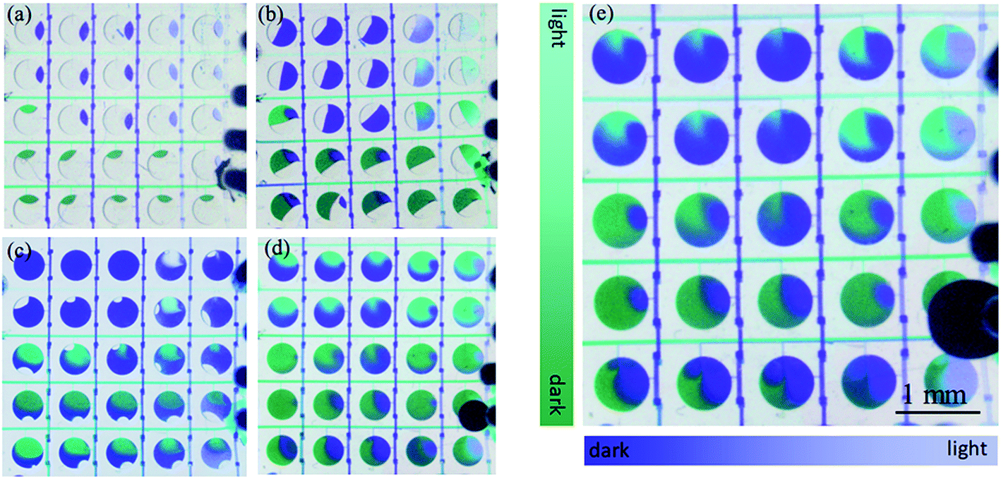Fig. 4 Using ink dye to show the whole process of 2D gradient generation. (a–d) The gradient is generally established, blue and green ink dye entering the chamber successively according to the chambers’ distance from their respective inlets. (e) The established gradient clearly shows the gradual change of the color ratio that implies they are of different concentration.

Results and analysis

The result of the ink dye experiment is observed using an optical microscope. The result of the fluorescein dye experiment is first observed using an optical microscope and then quantitatively analyzed using confocal microscopy. It should be noted that the normal ink dye is used only to qualitatively demonstrate the process of generation of a concentration gradient. Since the illumination condition could vary from time to time, reading the RGB value from the conventional ink dye could not be used as a reliable method to quantify the concentration. Also, the limitations of using Rhodamine B in our PDMS-based device should be addressed, for its absorption of Rhodamine B could influence the concentration and thus the intensity of this fluorescent dye. It is eligible to provide a reference value to allow us to compare the relative intensity horizontally at the same time,^23–26 such as, in our case, from chamber to chamber. However, this could introduce errors if monitoring the changing of intensity with time, i.e. comparing vertically.^27,28 In these cases, certain coating procedures would be necessary.

Using the ink dye, the process of gradient generation is clearly observed under an optical microscope (Fig. 4). In the beginning, the green dye occupies the diagonal lower-left chambers and the blue dye occupies the diagonal upper-right part (Fig. 4a). Considering the fact that the closer to the inlet, the larger the pumping pressure is, this phenomenon in the beginning could be attributed to the different distances from chambers to inlets. For example, the inlets of the blue dye are on the upper side, hence for chambers that are closer to the upper side and further from the left side (the inlets of the green dye), the blue dye will enter them first while the green dye is kept at their entrances. The same argument applies for the green dye, which occupies the diagonal lower-left chambers in the beginning, whose inlets are on the left side. After this initial stage, the two analytes enter the same chamber successively (Fig. 4b), as the infusion continues (Fig. 4c and d), two analytes will finally both enter the same chamber and form fine mixtures of different concentrations (Fig. 4e).

To systematically investigate the capability of the proposed 2D gradient generator, fluorescent dye was adopted for analyzing the intensity of each individual unit, and this could quantitatively reflect the corresponding concentrations in the mixtures. After the chip is adjusted to a stable state, it is then transferred to a confocal microscope for fluorescence image capture. Each individual chamber was recorded in sequence and then the pictures for individual chambers were stitched together to restore the whole intensity profile of the chip. ImageJ was used to quantitatively analyze the intensities in order to characterize the generated concentration gradient separately.

As can be seen from the intensity distribution at the stable state, it could be concluded that the 2D concentration gradient is successfully established (Fig. 5a and c). There are some fluctuations among the chambers of the same concentration (i.e. the same rows for Rhodamine B and the same columns for FITC). This is due to the delay of two analytes entering the same chamber as explained above. This problem could be compensated for more or less by reducing the height of the guide channel according to our trial experiment. Actually, it is the reason we take the trouble to spin coat three layers of photoresist of different heights. The highest layer, which consists of some pillars, is for penetrating the thin film to build the ladder, the middle height main channel is just a conventional flow path of an applicable height, and the purposefully lowered nozzle-like guide channel is to reduce the delay effect to a moderate level, without which the delay problem would be more severe than now according to our trials. The intensities of Rhodamine B and FITC show obvious trends of dropping down in intensity, implying a concentration gradient is established along their respective directions (Fig. 5b and d). The images of the two different fluorescent dyes are recorded simultaneously under a confocal microscope by setting up two receiving windows. Each receiving window is adjusted such that only the emitted light from the excited fluorescein dye of the target wavelength is recorded. Therefore, from these two figures showing the fluorescein dye 1D gradient separately (Fig. 5a and c), one could conclude that a 2D concentration gradient is well established.

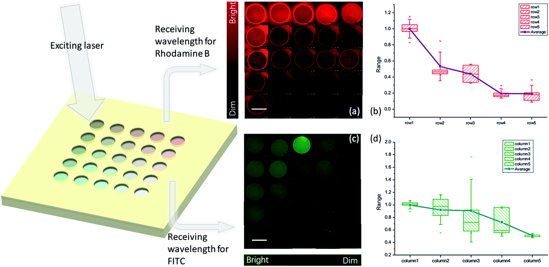Fig. 5 Fluorescent infusion and intensity analysis. (a) The Rhodamine B distribution observed using confocal microscopy chamber-by-chamber and then stitched together. (b) The line represents the normalized by largest average intensity of Rhodamine B changing from the 1st row to the 5th row. The box chart includes data between the lower quartile and upper quartile, showing the main distribution of concentrations. The whiskers represent the standard deviation. (c) The FITC distribution observed using confocal microscopy and processed the same as in the Rhodamine B case. (d) The line represents the normalized by largest average intensity of FITC changing from the 1st column to the 5th column. The box chart includes data between the lower quartile and upper quartile, showing the main distribution of concentrations. The whiskers represent the standard deviation. The scale bars are 1 mm.

For this typical demonstration, the flow rate of the fluorescent dyes is 1 ml h⁻¹ and that of DI water is 0.8 ml h⁻¹, as elaborated in the experimental section. To generate the customized concentration combinations on demand, it is necessary to generate the target two 1D gradients. From the study that describes the 1D concentration gradient generator,¹³ the concentration could be tuned. To adapt it to our scenario by changing Q_dye/Q_water, the respective outcome normalized concentration could be adjusted between 0∼1 and so can the concentration profile, which also varies with different combinations of Q_dye/Q_water. In the shown figure, there is a discrepancy between the shape of the trend for these two dyes. This could be attributed to fabrication errors when aligning the different layers. A biased alignment that favors one direction could give rise to a pressure environment that is different and complicated for both fluorescent dyes. Due to the use of manual alignment it is difficult to reach perfection, and hopefully in future versions with better aligning instruments this issue could be resolved.

Also, since this device has a nozzle-like branch channel, the shear force could be kept outside the chamber and has little effect inside the chamber, which is compatible with situations requiring a low shear force, like cell cultures. If the chip is used for screening functions, for instance screening the best combination of drugs for cells, a typical process could be conducted as follows: first the cells are introduced into the chambers using pumps and syringes before infusing drugs. Then the cells are cultured for two or three days to provide them sufficient time to attach to the chamber walls. Next we could use buffer to flush away the cells that are not tied to the wall of chamber. We then culture the cells until they are living stably in the chambers, and the combinations of different concentrations of the two drugs could be infused into the chamber according to what we have described in our manuscript to screen the best combination of drugs for the cells. During the infusion, since the cells are kept inside the chambers, they are free from the shear forces that come along with the fluid flow that could potentially flush them off the sidewalls of the chambers.

In addition, the combination of different analytes implies a mixing process, which would commonly raise concerns regarding the low mixing efficiency inside microfluidic devices. Here, we did not embed a mixing part due to its marginal contribution in our chip. A detailed discussion of this can be found in ESI 1 and 2.†

Conclusions

In this work, we have designed and demonstrated a valve-free 2D concentration gradient generator, for the formation of combinatorial diluted concentrations with two different analytes. This 2D concentration gradient generator works without any peripheral control components except for the pumps used for infusion, shedding light on possible options for making microfluidic chips closer to portable devices. The use of multilayer chip fabrication in the flow path design of a complicated, high flux function chip could save space, in order to keep the chip small, tightly packed, and highly integrated. While a chip alone can do only very limited things, plus the inevitability of using an external control method when loading samples, the idea of modifying the flow path or shaping the geometry of the channel may be a more intrinsic way of building up a chip. We believe that the presented device could have potential applications in drug screening, condition screening, etc. with a simple operating platform.

Acknowledgements

The authors would like to acknowledge the support of Hong Kong RGC Grants HKUST 16219216 and NSFC grant no. 11290165.

References

1. A. G. Toh, Z. Wang, C. Yang and N.-T. Nguyen, Microfluid. Nanofluid., 2014, 16, 1–18.
2. B. Zhou, W. Xu, A. A. Syed, Y. Chau, L. Chen, B. Chew, O. Yassine, X. Wu, Y. Gao and J. Zhang, Lab Chip, 2015, 15, 2125–2132.
3. C. L. Hansen, E. Skordalakes, J. M. Berger and S. R. Quake, Proc. Natl. Acad. Sci. U. S. A., 2002, 99, 16531–16536.
4. P. Yager, T. Edwards, E. Fu, K. Helton, K. Nelson, M. R. Tam and B. H. Weigl, Nature, 2006, 442, 412–418.
5. G. M. Walker, J. Sai, A. Richmond, M. Stremler, C. Y. Chung and J. P. Wikswo, Lab Chip, 2005, 5, 611–618.
6. J.-Y. Cheng, M.-H. Yen, C.-T. Kuo and T.-H. Young, Biomicrofluidics, 2008, 2, 024105.
7. W. Saadi, S.-J. Wang, F. Lin and N. L. Jeon, Biomed. Microdevices, 2006, 8, 109–118.
8. M. Skolimowski, M. W. Nielsen, J. Emnéus, S. Molin, R. Taboryski, C. Sternberg, M. Dufva and O. Geschke, Lab Chip, 2010, 10, 2162–2169.
9. B. G. Chung, L. A. Flanagan, S. W. Rhee, P. H. Schwartz, A. P. Lee, E. S. Monuki and N. L. Jeon, Lab Chip, 2005, 5, 401–406.
10. D. Irimia, D. A. Geba and M. Toner, Anal. Chem., 2006, 78, 3472.
11. N. L. Jeon, S. K. Dertinger, D. T. Chiu, I. S. Choi, A. D. Stroock and G. M. Whitesides, Langmuir, 2000, 16, 8311–8316.
12. F. Lin, W. Saadi, S. W. Rhee, S.-J. Wang, S. Mittal and N. L. Jeon, Lab Chip, 2004, 4, 164–167.
13. B. Zhou, W. Xu, C. Wang, Y. Chau, X. Zeng, X.-X. Zhang, R. Shen and W. Wen, Microfluid. Nanofluid., 2015, 18, 175–184.
14. B. Hong, P. Xue, Y. Wu, J. Bao, Y. J. Chuah and Y. Kang, Biomed. Microdevices, 2016, 18, 1–8.
15. J. Atencia, G. A. Cooksey and L. E. Locascio, Lab Chip, 2012, 12, 309–316.
16. J. Atencia, J. Morrow and L. E. Locascio, Lab Chip, 2009, 9, 2707–2714.
17. J. Kim, D. Taylor, N. Agrawal, H. Wang, H. Kim, A. Han, K. Rege and A. Jayaraman, Lab Chip, 2012, 12, 1813–1822.
18. D. An, K. Kim and J. Kim, Biomol. Ther., 2014, 22, 355.
19. Y.-H. Jang, M. J. Hancock, S. B. Kim, Š. Selimović, W. Y. Sim, H. Bae and A. Khademhosseini, Lab Chip, 2011, 11, 3277–3286.
20. C. Neils, Z. Tyree, B. Finlayson and A. Folch, Lab Chip, 2004, 4, 342–350.
21. B. R. Schudel, C. J. Choi, B. T. Cunningham and P. J. Kenis, Lab Chip, 2009, 9, 1676–1680.
22. M. Zhang, J. Wu, L. Wang, K. Xiao and W. Wen, Lab Chip, 2010, 10, 1199–1203.
23. K. P. Kim, Y.-G. Kim, C.-H. Choi, H.-E. Kim, S.-H. Lee, W.-S. Chang and C.-S. Lee, Lab Chip, 2010, 10, 3296–3299.
24. Y. Du, M. J. Hancock, J. He, J. L. Villa-Uribe, B. Wang, D. M. Cropek and A. Khademhosseini, Biomaterials, 2010, 31, 2686–2694.
25. T. Kim, M. Pinelis and M. M. Maharbiz, Biomed. Microdevices, 2009, 11, 65.
26. E. Choi, H.-K. Chang, C. Y. Lim, T. Kim and J. Park, Lab Chip, 2012, 12, 3968–3975.
27. D. Erickson, X. Liu, R. Venditti, D. Li and U. J. Krull, Anal. Chem., 2005, 77, 4000–4007.
28. R. Samy, T. Glawdel and C. L. Ren, Anal. Chem., 2008, 80, 369–375.

---

Footnote

† Electronic supplementary information (ESI) available. See DOI: 10.1039/c7ra02139a

---