
 Open Access Article
 This Open Access Article is licensed under a
 Creative Commons Attribution 3.0 Unported Licence
Dispersion of non-covalently modified graphene in aqueous medium: a molecular dynamics simulation approach†‡
Aditya Kulkarni,
Nabaneeta Mukhopadhyay ,
Arup R. Bhattacharyya and
Ajay Singh Panwar*
,
Arup R. Bhattacharyya and
Ajay Singh Panwar*
Department of Metallurgical Engineering and Materials Science, Indian Institute of Technology Bombay, Powai, Mumbai – 400076, India. E-mail: panwar@iitb.ac.in
First published on 16th January 2017
Abstract
Molecular dynamics were used to simulate the dispersion of graphene in aqueous medium in the presence of a novel organic modifier, sodium salt of 6-amino hexanoic acid (Na-AHA), which non-covalently modifies the graphene surfaces. The modifier molecule contains an ionizable carboxylate head group and an aliphatic tail. The extent of dispersion was estimated by calculating the potential of mean force (PMF) as a function of increasing concentration of the modifier using the thermodynamic perturbation method in conjunction with molecular dynamics simulations. With increasing concentration of the modifier, the PMF changed from a short-range strong attraction to a long-range repulsion at higher modifier concentrations. The simulation results clearly show the adsorption of modifier molecules at the graphene–water interface, which in turn causes the graphene surfaces to acquire a negative charge. Further, the development of a negative electric potential at the graphene surfaces induces a long-range electrostatic repulsion between the graphene sheets, clearly pointing to an electrostatic stabilization of Na-AHA modified-graphene in aqueous medium.
Introduction
Graphene has been widely used in suspensions, polymer based solutions, melts and composites1–4 because of its excellent mechanical, thermal, and electronic properties, low electrical percolation thresholds and high aspect ratio. The incorporation of graphene as the dispersed phase in various host matrices is complicated by high aspect ratios and extremely high surface areas, resulting in extremely high attraction energies (as high as 500 eV μm−1).5 Thus, the processing of a graphene-based polymer composite system is complicated by agglomeration6–9 and poor polymer/graphene interfacial interactions.10,11 Non-covalent modification of the graphene surfaces is a versatile strategy for improving dispersion of graphene in host matrices (as opposed to covalent modification that can alter intrinsic properties).12,13 Surface modification is usually achieved through adsorption of either polymers or surfactants onto the graphene surfaces, which enable dispersion via long-range electrostatic or short-range steric interactions. In a polar medium (such as water), ionic surfactants and polyelectrolytes can be used as dispersants for electrostatically stabilizing graphene particles. Common surfactants, such as sodium dodecyl sulphate (SDS),14–16 are widely used for stabilizing dispersions in aqueous media. Often, preliminary dispersion of graphene in aqueous media is followed by their subsequent incorporation into polymer melts for processing of polymer nano-composites. In such applications, the surfactant/modifier can serve dual purposes of not only initially dispersing graphene, but may also contribute to improved interfacial compatibility at the graphene/polymer interface.The sodium salt of 6-amino hexanoic acid (Na-AHA), first developed by Kodgire et al.17 as a reactive modifier for carbon nanotubes (CNTs), leads to both improved CNT dispersion in water and exfoliated nanotube networks in polyamide 6 based blend systems during subsequent melt-mixing. The improved interaction of the CNTs with the polymer matrix is thought to arise from the melt–interfacial interactions involving amine groups present in the modifier. There are several reports of achieving lower electrical percolation threshold, improvement in blend microstructure and blend properties as a result of incorporation of Na-AHA modified multi-walled carbon nanotubes (MWCNTs) in various blend systems.18–26 The use of Na-AHA-like dispersant as a reactive modifier was extended to graphene-based polymer nanocomposite system where similar improvements in both graphene dispersion and the final nanocomposite properties were reported.24 Since the addition of Na-AHA as a modifier contributes positively to the final properties of the nanocomposite (unlike conventional surfactants, such as SDS, which can adversely affect the properties), it is important to examine the mechanism of dispersion of graphene in the presence of Na-AHA.
Such an investigation is ideally suited for treatment with molecular dynamics, which can answer several questions at the atomistic level relating to mechanistic aspects of dispersion of Na-AHA modified graphene sheets. The first issue is related to the partitioning of the Na-AHA molecules onto the graphene surface from the aqueous phase. Another unknown aspect is whether the graphene particles are stabilized primarily via electrostatic or steric interactions. Also, unlike SDS, which contains only one ionizable group, Na-AHA has two groups (carboxyl and amine groups at either ends), both or either of them could be ionized depending on solution pH.
There exist several simulation studies, where various aspects of dispersion of hydrophobic solutes (specifically, graphene, graphene oxide, or CNTs) have been investigated.27–36 When used in conjunction with free energy calculation methods, molecular dynamics simulations can be used to estimate free energy differences between states corresponding to different extents of dispersion. Specifically, aspects of dispersion related to solute wetting behaviour, surfactant adsorption and surfactant concentration have been explored using molecular dynamics simulations. Simulations of two CNTs in water revealed a continuous “wetting” or a “drying” of the interstice between the tubes depending on their initial spacing.37 Other molecular dynamics simulations have investigated the energetics of the transfer of surfactant molecules from the bulk solution phase to a solid solute surface,38 dependence of morphology of SDS surfactant aggregates on nanotube diameter,39 and CNT–CNT interactions in the presence of either surfactant40,41 or polymer molecules.42
Thermodynamic perturbation has been widely used to calculate the PMF as a function of distance between two hydrophobic solutes in a solvent for a variety of systems. Averages are performed over specific degrees of freedom corresponding to a particular state and the statistical data can be obtained from a MD simulation. In one of the earliest simulations, Linse43 has calculated the PMF between two benzene molecules in an aqueous solvent as a function of their relative orientations. Choudhury and Pettitt44–48 have extensively studied the hydration behaviour of two planar hydrophobic solutes in liquid water by calculating the PMF between them. In a series of papers, Eun and Berkowitz49–54 have employed thermodynamic perturbation to investigate the interaction between model lipid bilayers (phosphatidylcholine headgroups grafted to graphene plates).
In this report, we explore the effect of increasing concentration of Na-AHA on the dispersion of two graphene sheets (planar hydrophobic solutes) using molecular dynamics simulations and employ thermodynamic perturbation to calculate the PMF as a function of the separation distance between the two graphene sheets. Moreover, it was observed that the PMF changed from a short-range strong attraction for bare graphene surfaces, to an increasingly long-range repulsion upon addition of Na-AHA, which adsorbed onto the graphene surfaces. Further, we could find that the long-range repulsion was electrostatic in origin, which clearly suggested an electrostatic stabilization of Na-AHA-modified graphene dispersions. To the best of our knowledge, evidence of electrostatic stabilization of non-covalently modified hydrophobic nanoparticles has not been previously reported in the simulation literature. The remainder of the article is organized as follows. We provide the details of the simulation method in the following section. Our main results are presented and discussed in the Results and discussion section. Finally, we summarize and conclude the discussion in the Summary section.
Simulation method
Fig. 1 is a schematic of the simulation set-up with two graphene sheets of size 30 × 30 Å2 separated by a distance d along the X-axis. The two graphene sheets are modeled as rigid objects and are always oriented parallel to each other during the course of the simulations. These were solvated in a 50 × 50 × 60 Å3 box of TIP3P water molecules (at a density of 1 g cm−3) with periodic boundary conditions in all three directions. In addition, n molecules of the organic dispersant, Na-AHA, were also introduced in the space between the two graphene sheets. Since the dispersant molecule is a sodium salt of 6-amino hexanoic acid (the anionic component of the salt is abbreviated to AHA in the rest of the article), n number of Na+ counter-ions were also added to the simulation box. Thus, by varying n, we model the effect of varying relative concentrations of the dispersant, Na-AHA, with respect to graphene. Three values of n = 0, 6, 21 corresponding to Na-AHA concentrations of 0 M, 0.05 M and 0.16 M, respectively, were considered in the simulations. In all, the simulation box contains close to 14![[thin space (1/6-em)]](https://www.rsc.org/images/entities/char_2009.gif) 000 atoms. The CHARMM force-field was used to model all inter-atomic interactions in the simulation. Electrostatic interactions were evaluated using the particle–particle particle mesh Ewald summation with an accuracy of 10−4. Lennard-Jones interactions were used to model the other non-bonded interactions (including van der Waals) between atoms. Inner and outer cut-offs of 8 and 10 Å respectively, were used for both electrostatic and Lennard-Jones interactions. A switching function was used to smoothly bring the energies and forces to zero between the inner and outer cut-offs. Simulations were carried out in an NPT ensemble at a temperature of 300 K and a pressure of 1 atmosphere. A Langevin thermostat was used with a characteristic damping time constant of 100 fs to maintain the system temperature. A Berendsen barostat with a time constant of 1000 fs was used for maintaining the pressure. All simulations were implemented in the open-source package LAMMPS55 (http://lammps.sandia.gov). A timestep of 1 fs and an equilibration time of 1 ns were used for simulations at any given separation of d. The duration of the equilibration time is similar to previously reported studies employing molecular dynamics and thermodynamic perturbation, which have typically used equilibration times in the range of 100–500 ps.43,44,49 The separation d was varied between 4–30 Å for all simulations.
000 atoms. The CHARMM force-field was used to model all inter-atomic interactions in the simulation. Electrostatic interactions were evaluated using the particle–particle particle mesh Ewald summation with an accuracy of 10−4. Lennard-Jones interactions were used to model the other non-bonded interactions (including van der Waals) between atoms. Inner and outer cut-offs of 8 and 10 Å respectively, were used for both electrostatic and Lennard-Jones interactions. A switching function was used to smoothly bring the energies and forces to zero between the inner and outer cut-offs. Simulations were carried out in an NPT ensemble at a temperature of 300 K and a pressure of 1 atmosphere. A Langevin thermostat was used with a characteristic damping time constant of 100 fs to maintain the system temperature. A Berendsen barostat with a time constant of 1000 fs was used for maintaining the pressure. All simulations were implemented in the open-source package LAMMPS55 (http://lammps.sandia.gov). A timestep of 1 fs and an equilibration time of 1 ns were used for simulations at any given separation of d. The duration of the equilibration time is similar to previously reported studies employing molecular dynamics and thermodynamic perturbation, which have typically used equilibration times in the range of 100–500 ps.43,44,49 The separation d was varied between 4–30 Å for all simulations.
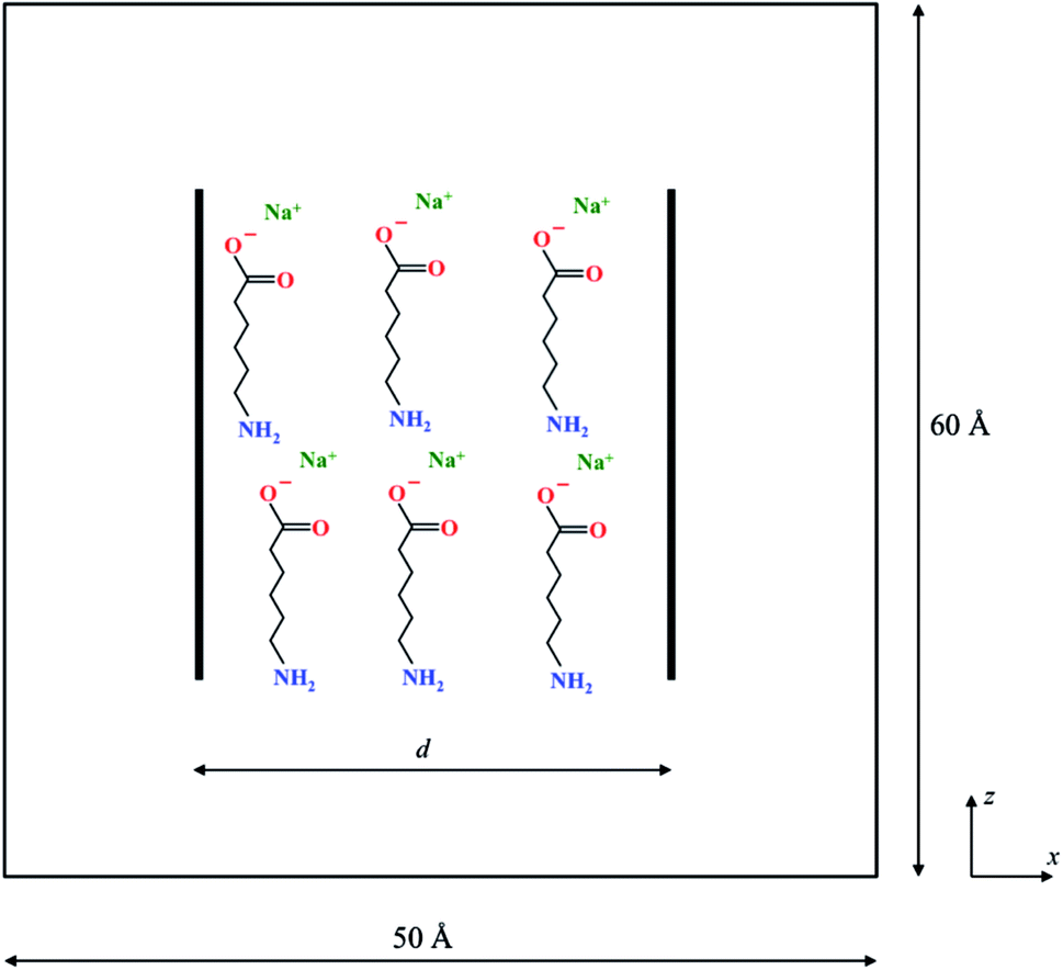 | ||
| Fig. 1 Schematic representation of the simulation box containing two graphene sheets solvated in water and arranged parallel to each other at a separation d. To this, nNa-AHA modifier molecules are added. | ||
Thermodynamic perturbation was used to calculate the potential of mean force between the two graphene sheets. According to the perturbation theory developed initially by Zwanzig,56 the free energy difference between an initial state “0” and a slightly perturbed state “1” is given by,
 | (1) |
| d0(λi) = dmin0 + λi(dmax0 − dmin0) | (2) |
 | (3) |
However, it should be noted that the potential of mean force so obtained is only a relative measure since only free energy differences can be obtained using this method. The potential of mean force was chosen to be zero at the largest separation considered.
Results and discussion
Fig. 2 shows the total calculated potential of mean force (PMF) for the system for varying dispersant concentrations of n = 0, 6, and 21. The case of n = 0 models the interactions between two “bare” or “unmodified” graphene sheets in water. The PMF plot for this case shows a deep potential well of nearly −400 kcal mol−1 at 3.9 Å separation (see inset) indicating a strong attraction between the graphene sheets. Further, the interaction quickly goes to zero at a separation of around 12 Å indicating a short-range interaction between the graphene sheets. These observations are consistent with the expected behaviour of an hydrophobic solute in an aqueous environment. Hydrophobic solutes are expected to aggregate in water due to strong attractive interactions between them. In addition, a small positive peak of nearly 20 kcal mol−1 is observed at approximately 9 Å separation. This peak occurs for all three values of n and can be ascribed to oscillatory solvation forces arising due to the ordering of water molecules between the graphene sheets.57 As the concentration of dispersant is increased, it is seen that the interaction changes completely from a short-range attractive interaction to a longer-range repulsive interaction. The PMF curves for both n = 6 and n = 21 show an entirely repulsive behaviour for all separation distances between the two graphene sheets. The peak value of the repulsive interaction increases from ≈40 kcal mol−1 for n = 6 to ≈55 kcal mol−1 for n = 21. Also, the interaction is more repulsive for n = 21 than n = 6 for all separations. In both cases, and in contrast with the n = 0 case, the interaction stays significant for larger separations, and approaches zero close to 22 Å. Thus, the range of interaction increases by nearly 10 Å for both n = 6 and n = 21 when compared to the n = 0 case.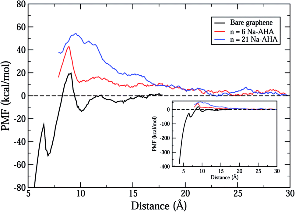 | ||
| Fig. 2 The total calculated PMF as a function of inter-sheet distance, d, between the two graphene sheets for the three cases of n = 0 (black) representing bare graphene sheets, n = 6 (red), and n = 21 (blue). The inset extends the distance axis to less than 5 Å showing that the PMF for the bare graphene surfaces has a minima of approximately −400 kcal mol−1. | ||
Thus, the PMF plots for finite dispersant concentrations in Fig. 2 clearly suggest two important effects. First, an increase in the strength of repulsion with an increase in dispersant concentration indicates that graphene surfaces are modified by possible adsorption of Na-AHA onto graphene surfaces. Second, the long-range character of the PMF for n = 6 and 21 is a strong indication of an electrostatic repulsion between the two graphene sheets. The following set of results explore this hypothesis.
In Fig. 3(a)–(c), we plot the important contributions to the total PMF of the system for different values of n. The “components” of the PMF were calculated on the basis of the pair interaction energies for different groups of atoms, corresponding to graphene and water (Fig. 3(a)), the two graphene sheets (Fig. 3(b)), graphene and dispersant molecules (Fig. 3(c)). One should note that the graphene refers to the unmodified graphene sheet consisting of only carbon atoms. The interaction between graphene and water becomes increasingly repulsive as n increases. For n = 0, the PMF fluctuates around zero and has two minima at d = 7 and 10 Å respectively. This could be due to packing of layers of water molecules between the graphene sheets. An increase in the strength of the PMF with n would be a direct result of an increase in the number of graphene–water pairs that are used to compute the PMF, suggesting that more water molecules entered the region between the graphene sheets as more dispersant molecules were added. This behaviour indicates that the graphene surfaces are being modified by dispersant molecules, and consequently becoming hydrophilic. Since graphene is a hydrophobic solute, the PMF would become increasingly repulsive for increasing numbers of graphene–water contacts. Hence, there is a strong indication of adsorption of AHA chains onto the graphene surfaces, the latter being rendered hydrophilic due to the presence of the carboxylate groups.
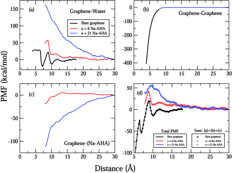 | ||
| Fig. 3 Plot showing important contributions to the total PMF corresponding to (a) graphene–water, (b) graphene–graphene, (c) graphene–Na-AHA, respectively. The plot in (d) represents the sum of contributions from (a), (b) and (c) (open circles) with the total PMF from Fig. 2 (solid lines). For the case of n = 0 (bare graphene), the sum includes only contributions from (a) and (b). The different concentrations are represented by the colors, black (n = 0), red (n = 6), and blue (n = 21) for all plots (a)–(d). For all concentrations in (d), the two curves lie on top of each other, indicating that the total PMF is represented by the sum of the three components. | ||
In Fig. 3(b), the PMF for graphene–graphene pairs is calculated. It is invariant with changes in n, and decreases monotonically with decrease in d. This is expected because the graphene–graphene interaction should not change with increasing n, and should be strongly attractive over short ranges. The PMF shows a deep minimum of −400 kcal mol−1 at 3.9 Å and rapidly goes to zero at around 8 Å separation. The graphene–graphene interaction seems to be the major contribution to the total calculated PMF for the n = 0 case in Fig. 2.
The first evidence for adsorption of the AHA molecules onto the graphene surfaces comes from the corresponding PMF plot of graphene–Na-AHA (Fig. 3(c)). For n = 6, the PMF is close to zero for larger separations, but starts becoming negative at around 12 Å separation and drops down further to −20 kcal mol−1 at 7 Å. This corresponds to an attractive interaction between the dispersant molecules and the graphene surfaces. The AHA backbone is comprised of 5CH2 groups which have an attractive interaction with the graphene surface, leading to their adsorption onto the graphene surfaces. When the concentration of dispersant molecules increases to n = 21, PMF values are found to be negative over the entire range of d. The PMF decreases monotonically from zero at 30 Å to −120 kcal mol−1 at 7 Å. The value at 7 Å separation is nearly six times larger than the PMF value for the n = 6 case. The larger negative PMF for n = 21 is a result of a greater number of Na-AHA molecules being adsorbed onto the graphene surfaces, because more are present at higher concentrations. Hence, an increased adsorption of AHA molecules onto graphene makes the graphene surface more hydrophilic, which increases the local concentration of water molecules in the vicinity of the graphene surfaces. This should lead to a corresponding increase in the graphene–water PMF plot, which is exactly what we observe in Fig. 3(a).
In order to reiterate that the “components” in Fig. 3(a)–(c) are the most important contributors to the PMF, we plot in Fig. 3(d), the sum of these three contributions (represented by open circles) and the total PMF (from Fig. 2 and represented by solid lines) for all three values of n. For each case, we find that the total PMF is described exactly by the sum of the three components in Fig. 3(a)–(c) (the two curves lie on top of each other). Of course, for the case of n = 0, the sum includes only the graphene–water and graphene–graphene contributions. The fact that the total PMF can be expressed as an exact sum of the three PMF “components” is an important result, which strongly suggests that the dispersion of graphene in water is controlled by the interfacial interaction between the graphene and Na-AHA molecules. In their simulations of interactions between model lipid bilayers comprised of zwitterionic and charged functional groups, Eun and Berkowitz54 showed that the PMF was composed of direct interactions and water-mediated interactions between the plates. Whereas, entropic contributions to the solvent-mediated interactions led to attraction, enthalpic contributions to solvent-mediated interactions led to repulsion between the model bilayers.
In Fig. 4(a)–(c), we plot the distribution of water molecules in the box along the X-axis at separations of 10 Å, 20 Å, and 30 Å, respectively. The number density values for water were calculated for volumes that were slices in the Y–Z plane with thicknesses of Δx = 0.1 Å. For the three values of d considered here, the graphene sheets were located at x = ±5 Å, x = ±10 Å, and x = ±15 Å in Fig. 4(a)–(c), respectively. In the space between the graphene sheets, the water density seems to decrease with increasing n, which happens because water molecules are displaced by Na-AHA molecules with increase in n. At first glance, this result seems to counter our claim of increased graphene–water repulsion with increasing n from Fig. 3(a). However, a more careful observation of water–graphene interactions presented in Fig. S1 (see ESI†) for the test case of d = 10 Å supports our claim of increased water–graphene repulsion with increasing n. Fig. S1(a)† replots the water density distributions from Fig. 4(a) showing that water density between the graphene sheets decreases with increasing n. A direct calculation of the van der Waals energy between the water molecules and the graphene sheets is presented in Fig. S1(b)† for −8.5 ≤ x ≤ 8.5. Since the van der Waals diameter of an oxygen–carbon pair is approximately 3.5 Å, interactions beyond 3.5 Å on the outside of the graphene sheets are ignored. In the space between the graphene sheets, the van der Waals interaction energy becomes less attractive (or more repulsive) with increase in n. This is also confirmed in Fig. S1(c)† which plots the time dependence of the graphene–water interaction energy over the course of the simulation for the three values of n. The results of another simulation presented in Fig. S2 (see ESI†) for the case of a single 50 × 50 Å2 graphene sheet, with 21 Na-AHA molecules adsorbed on both sides of the sheet, also show that the water–graphene interaction indeed becomes more repulsive with increasing n. This is the primary cause for the stabilization of graphene sheets in the presence of the dispersant Na-AHA, and is indicated by an overall repulsive PMF (Fig. 2).
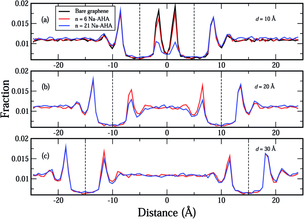 | ||
| Fig. 4 Plots of fractional number density of water molecules in the simulation box along the X-axis (separation axis) for (a) d = 10 Å, (b) d = 20 Å, and (c) d = 30 Å, respectively. The vertical dashed lines indicate the location of the two graphene sheets in the simulation box for the corresponding separation distances in (a)–(c). The different concentrations are represented by the colors, black (n = 0), red (n = 6), and blue (n = 21) for all plots (a)–(c). For reference, the simulation box extends from −25 Å to 25 Å along the X-axis. | ||
The density profiles of carboxylate and amine headgroups at 10 Å and 20 Å separations for both n = 6 and 21 are shown in Fig. 5. The density profiles indicate that the dispersant molecules are mostly confined to the space present between the graphene sheets. Also, the density profiles of the carboxylate and amine headgroups consistently show increased presence around the graphene sheets. This explains the increased amount of water in the immediate vicinity of the graphene sheets. In combination with an attractive PMF for graphene–dispersant molecules (Fig. 3(c)), these profiles provide strong evidence of the adsorption of dispersant molecules onto the surface of the graphene sheets. The distribution of the counter ions has been described in Fig. 6. The Na+ ions lie completely between the two sheets for all values of n. The extremely high hydration of the hard sodium ions, coupled with their affinity for the carboxylate group, constrains them to remain localized between the sheets and in the vicinity of the dispersant molecule. The presence of the counter-ions between the sheets draws more water molecules towards the graphene sheets, thus contributing to further stabilization.
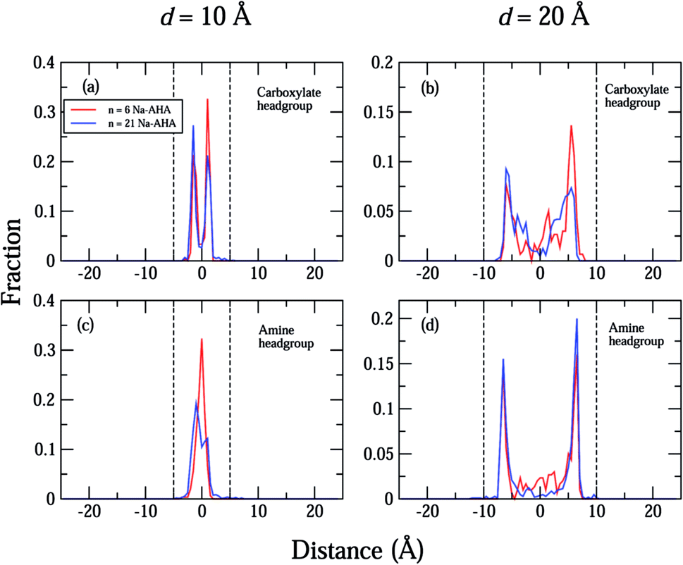 | ||
| Fig. 5 Plots of respective fractional number densities, in the simulation box, of carboxylate headgroups along the X-axis (separation axis) for (a) d = 10 Å, (b) d = 20 Å, and amine headgroups along the X-axis (c) d = 10 Å, and (d) d = 20 Å. The vertical dashed lines indicate the location of the two graphene sheets in the simulation box for the corresponding separation distances in (a)–(d). The different concentrations are represented by the colors, red (n = 6), and blue (n = 21) for all plots (a)–(d). For reference, the simulation box extends from −25 Å to 25 Å along the X-axis. | ||
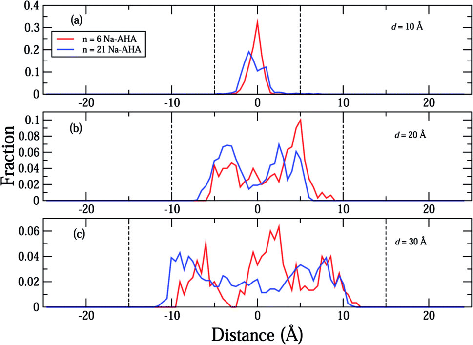 | ||
| Fig. 6 Plots of respective fractional number densities of Na+ counter-ions in the simulation box along the X-axis (separation axis) for (a) d = 10 Å, (b) d = 20 Å, and (c) d = 30 Å. The vertical dashed lines indicate the location of the two graphene sheets in the simulation box for the corresponding separation distances in (a)–(c). The different concentrations are represented by the colors, red (n = 6), and blue (n = 21) for all plots (a)–(c). For reference, the simulation box extends from −25 Å to 25 Å along the X-axis. | ||
Fig. 7 shows the average orientation of the hydrophobic AHA backbone (comprised of 5CH2 groups) and the negatively charged carboxylate head group of the dispersant molecules with respect to the graphene sheets. In order to evaluate this, the angles between the normal to the sheets and vectors parallel to the hydrophobic and hydrophilic parts of the surfactant molecules were evaluated. It can be seen that the hydrophobic AHA backbone is almost parallel to the graphene sheets (Fig. 7(a)) suggesting that the adsorption of the AHA molecule onto the graphene sheet is effected via the CH2 groups. Moreover, the hydrophilic part of the dispersant makes an angle of around 110 degrees with the normal (Fig. 7(b)), which is close to the bond angle value. This shows that the carboxylate group points away from the graphene, as would be expected for a hydrophilic functional group. Thus, the graphene surface is functionalized via adsorption of the (CH2)5 backbone and consequently rendered hydrophilic by the ionization of the carboxylate groups.
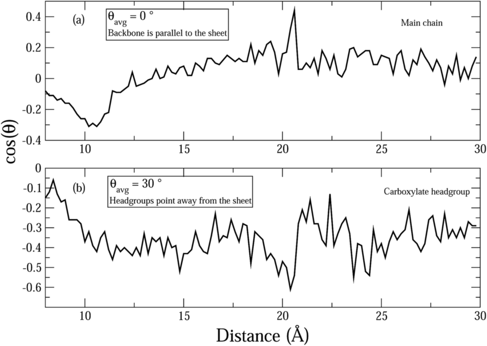 | ||
| Fig. 7 Figure showing the average orientation as a function of the inter-plate separation, d, for (a) the main chain of the Na-AHA molecule, and (b) the carboxylate headgroup, respectively, for the Na-AHA concentration of n = 21. | ||
The final piece of the puzzle is the long-range repulsive behaviour of the PMF in Fig. 2 for finite dispersant concentrations (n = 6, 21). For the case of n = 21 and d = 30 Å, we show the electric potential map in the X–Z plane at Y = 22.5 Å in Fig. 8(a). The electric potential map has been obtained using the PME Electrostatics module within the Visual Molecular Dynamics (VMD) package.58 Visually, one can distinguish regions with negative values of the electric potential in the proximity of the graphene sheets (red coloured regions). In contrast, regions with positive values of the electric potential are found away from the graphene surfaces in the bulk. A plot of the electric potential along the X-direction (Fig. 8(b)) in the middle of the plane proves this. In the region between the graphene sheets located at x = ±15 Å, the electric potential rises from −0.025 V at x ≈ −10 Å, to 0.225 V at x ≈ 0 Å, and drops back to approximately zero at x ≈ 10 Å. This shows conclusively that the regions immediately next to the graphene sheets are negatively biased with respect to the potential at the mid-point. Though the graphene sheets are located at x = ±15 Å, we need to account for the van der Waals diameter of the graphene carbon atoms and the thickness of the adsorbed (CH2)5 backbone of the AHA molecule to estimate the locations of the negatively charged carboxyl groups from x = ±15 Å. This distance is estimated to be between 5–7 Å, which is consistent with the location of the two minima close to x ± 10 Å. Thus, Fig. 8(b) shows conclusively that the adsorption of AHA molecules leads to a negative surface potential on the graphene surfaces with respect to the aqueous environment. This leads to the emergence of a long-range electrostatic interaction between the graphene surfaces, and further contributes to their stabilization in aqueous media.
 | ||
| Fig. 8 (a) The electric potential map in the X–Z plane at Y = 22.5 Å, where the red and blue regions indicate negative and positive values of the electric potential, respectively, corresponding to the Na-AHA concentration of n = 21 and a separation of d = 30 Å. The scale bar shows the electric potential in units of kBT/e, hence the numbers need to be multiplied by approximately 0.025 to obtain values in volts. (b) A plot of the electric potential along the X-direction in the middle of the plane in (a) indicates that the surface potential of graphene sheets is nearly −0.225 V with respect to the potential at the mid-point between the sheets. | ||
Summary
We have utilized MD simulations and thermodynamic perturbation theory to calculate the potential of mean force as a function of inter-plate distance between two graphene sheets in water, and in the presence of a novel modifier, Na-AHA. Simulations have been carried out for varying concentrations of Na-AHA molecules. Our simulations clearly indicate that Na-AHA molecules lead to repulsive interactions between the two hydrophobic graphene sheets in aqueous medium. Specifically, our results show the following:• Addition of Na-AHA molecules to the simulation box led to a qualitative change in the nature of interactions between the two graphene sheets. The interaction changed from a strong short-range attraction for the case of bare graphene sheets in water, to a long-range repulsion upon addition of Na-AHA molecules to the system. The addition of the Na-AHA molecules also increased the range of the potential by nearly 10 Å when compared to the case when no dispersant molecules are present. In earlier simulations of CNT–CNT interactions in water in the presence of SDS molecules, Uddin et al. found an increase in the range of the potential of mean force (PMF) with increase in the concentration of SDS molecules (from zero to four to ten).40,41 In addition, a decrease in the well-depth of the PMF with respect to that of the unmodified CNTs was observed, which was attributed to an increase in the steric size of the CNTs upon adsorption of the SDS molecules. However, no signature of long-range electrostatic stabilization, expected due to the presence of the ionic carboxylate group on SDS, was observed in the PMF.
• Our simulation studies showed that graphene surfaces are non-covalently modified by the adsorption of the Na-AHA molecules onto graphene surfaces, and that the adsorption took place via the aliphatic backbone comprising of 5CH2 groups. The energetics of the process of transfer of a single surfactant molecule from the bulk solution phase to a solid solute surface has been simulated earlier by Xu et al.38 It was found that the free energy profile for surfactant approaching the surface is determined by a remarkably fine balance between the opposing entropy and enthalpy terms, and that the stabilization of surfactant adsorption behaviour is enthalpically dominated. Further, we find that the adsorption of the AHA molecules onto the graphene sheets could draw in more water molecules in the vicinity of the graphene sheets, rendering the initially hydrophobic graphene surfaces hydrophilic. This could happen because of the hydration of the polar carboxylate groups present in the Na-AHA molecules.
• Finally, a calculation of the electric potential map in the simulation box clearly showed that the Na-AHA-modified graphene sheets were negatively charged with respect to the mid-plane in the inter-plate region. The surface potential was approximately −0.225 V with respect to the “bulk”, arising from the presence of the negatively charged carboxyl groups of Na-AHA. Thus, we could show that the long-range repulsion between the two Na-AHA-modified graphene sheets is due to an electrostatic interaction.
Detailed experiments in the past have shown that Na-AHA was very effective in stabilizing aqueous dispersions of both multi-walled carbon nanotubes23 and graphene.24 However, the mechanisms of both non-covalent modification by Na-AHA and the subsequent dispersion of graphene particles (or CNTs) were not understood clearly. Our simulations could provide useful insight into the dispersion mechanism, clearly indicating that the dispersions were electrostatically stabilized upon adsorption of the AHA molecules. In addition, our results are also relevant for other amphiphilic dispersants, such as SDS, which contain an ionizable functional group. We should expect a qualitatively similar behaviour for this category of dispersants. Further, recent experiments on the dispersion of Na-AHA modified MWCNTs (not reported yet) have shown that the dispersion quality depends strongly on the solvent pH. This could occur because of the ionization of the amine group in Na-AHA under low pH conditions, leading to a more complex dispersion mechanism. Molecular dynamics can be used to simulate the effect of pH, and the comparison between experimental findings and simulations is the subject of another manuscript, which is currently under preparation. Thus, our MD simulations can, in principal, provide a qualitative stability map for different concentrations and pH conditions for a Na-AHA-type dispersant for graphene dispersions.
Acknowledgements
ASP would like to acknowledge Grant SR/S3/ME/0016/2011 from the Department of Science and Technology, Ministry of Science and Technology, India for funding support.References
- K. Wakabayashi, C. Pierre, D. A. Dikin, R. S. Ruoff, T. Ramanathan, L. C. Brinson and J. M. Torkelson, Macromolecules, 2008, 41, 1905–1908 CrossRef CAS.
- S. Park, J. An, I. Jung, R. D. Piner, S. J. An, X. Li, A. Velamakanni and R. S. Ruoff, Nano Lett., 2009, 9, 1593–1597 CrossRef CAS PubMed.
- H. Kim, A. A. Abdala and C. W. Macosko, Macromolecules, 2010, 43, 6515–6530 CrossRef CAS.
- J. R. Potts, S. Murali, Y. Zhu, X. Zhao and R. S. Ruoff, Macromolecules, 2011, 44, 6488–6495 CrossRef CAS.
- L. Girifalco, M. Hodak and R. S. Lee, Phys. Rev. B: Condens. Matter Mater. Phys., 2000, 62, 13104 CrossRef CAS.
- E. T. Thostenson, Z. Ren and T.-W. Chou, Compos. Sci. Technol., 2001, 61, 1899–1912 CrossRef CAS.
- J. Hilding, E. A. Grulke, Z. George Zhang and F. Lockwood, J. Dispersion Sci. Technol., 2003, 24, 1–41 CrossRef CAS.
- D. Paul and L. Robeson, Polymer, 2008, 49, 3187–3204 CrossRef CAS.
- P.-C. Ma, N. A. Siddiqui, E. Mäder and J.-K. Kim, Compos. Sci. Technol., 2011, 71, 1644–1651 CrossRef CAS.
- S. Tjong, Mater. Sci. Eng., R, 2006, 53, 73–197 CrossRef.
- S. Pegel, P. Pötschke, G. Petzold, I. Alig, S. M. Dudkin and D. Lellinger, Polymer, 2008, 49, 974–984 CrossRef CAS.
- N. G. Sahoo, S. Rana, J. W. Cho, L. Li and S. H. Chan, Prog. Polym. Sci., 2010, 35, 837–867 CrossRef CAS.
- L. S. Fifield, L. R. Dalton, R. S. Addleman, R. A. Galhotra, M. H. Engelhard, G. E. Fryxell and C. L. Aardahl, J. Phys. Chem. B, 2004, 108, 8737–8741 CrossRef CAS.
- K. Yurekli, C. A. Mitchell and R. Krishnamoorti, J. Am. Chem. Soc., 2004, 126, 9902–9903 CrossRef CAS PubMed.
- M. J. O'connell, S. M. Bachilo, C. B. Huffman, V. C. Moore, M. S. Strano, E. H. Haroz, K. L. Rialon, P. J. Boul, W. H. Noon and C. Kittrell, et al., Science, 2002, 297, 593–596 CrossRef PubMed.
- C. Richard, F. Balavoine, P. Schultz, T. W. Ebbesen and C. Mioskowski, Science, 2003, 300, 775–778 CrossRef CAS PubMed.
- P. V. Kodgire, A. R. Bhattacharyya, S. Bose, N. Gupta, A. R. Kulkarni and A. Misra, Chem. Phys. Lett., 2006, 432, 480–485 CrossRef CAS.
- S. Bose, A. R. Bhattacharyya, R. A. Khare, A. R. Kulkarni, T. U. Patro and P. Sivaraman, Nanotechnology, 2008, 19, 335704 CrossRef PubMed.
- S. Bose, A. R. Bhattacharyya, A. R. Kulkarni and P. Pötschke, Compos. Sci. Technol., 2009, 69, 365–372 CrossRef CAS.
- S. Bose, A. R. Bhattacharyya, R. A. Khare, S. S. Kamath and A. R. Kulkarni, Polym. Eng. Sci., 2011, 51, 1987–2000 CAS.
- R. A. Khare, A. R. Bhattacharyya and A. R. Kulkarni, J. Appl. Polym. Sci., 2011, 120, 2663–2672 CrossRef CAS.
- A. V. Poyekar, A. R. Bhattacharyya, A. S. Panwar, G. P. Simon and D. S. Sutar, ACS Appl. Mater. Interfaces, 2014, 6, 11054–11067 CAS.
- J. Banerjee, A. S. Panwar, K. Mukhopadhyay, A. Saxena and A. R. Bhattacharyya, Phys. Chem. Chem. Phys., 2015, 17, 25365–25378 RSC.
- M. Sreekanth, A. S. Panwar, P. Pötschke and A. R. Bhattacharyya, Phys. Chem. Chem. Phys., 2015, 17, 9410–9419 RSC.
- S. Bose, A. R. Bhattacharyya, P. V. Kodgire, A. R. Kulkarni and A. Misra, J. Nanosci. Nanotechnol., 2008, 8, 1867–1879 CrossRef CAS PubMed.
- S. Bose, A. R. Bhattacharyya, R. A. Khare, A. R. Kulkarni and P. Pötschke, Macromolecular symposia, 2008, pp. 11–20 Search PubMed.
- M. K. Rana and A. Chandra, J. Chem. Phys., 2013, 138, 204702 CrossRef PubMed.
- P. Yang and F. Liu, J. Appl. Phys., 2014, 116, 014304 CrossRef.
- A. G. Hsieh, S. Korkut, C. Punckt and I. A. Aksay, Langmuir, 2013, 29, 14831–14838 CrossRef CAS PubMed.
- B. Sohrabi, N. Poorgholami-Bejarpasi and N. Nayeri, J. Phys. Chem. B, 2014, 118, 3094–3103 CrossRef CAS PubMed.
- T. A. Ho and A. Striolo, Mol. Simul., 2014, 40, 1190–1200 CrossRef CAS.
- A. Nicolaï, P. Zhu, B. G. Sumpter and V. Meunier, J. Chem. Theory Comput., 2013, 9, 4890–4900 CrossRef PubMed.
- T. Abi and S. Taraphder, Int. J. Comput. Theor. Chem., 2014, 1027, 19–25 CrossRef CAS.
- J. Marti, J. Sala and E. Guardia, J. Mol. Liq., 2010, 153, 72–78 CrossRef CAS.
- S. W. Han and J. Jang, Relation, 2006, 6, 2 Search PubMed.
- J. A. Garate, T. Perez-Acle and C. Oostenbrink, Phys. Chem. Chem. Phys., 2014, 16, 5119–5128 RSC.
- J. Walther, R. Jaffe, T. Halicioglu and P. Koumoutsakos, Center for Turbulence Research: Proceedings of the Summer Program, http://www.ctr.stanford.edu, 2000, pp. 5–20 Search PubMed.
- Z. Xu, X. Yang and Z. Yang, J. Phys. Chem. B, 2008, 112, 13802–13811 CrossRef CAS PubMed.
- N. R. Tummala and A. Striolo, ACS Nano, 2009, 3, 595–602 CrossRef CAS PubMed.
- N. M. Uddin, F. Capaldi and B. Farouk, J. Eng. Mater. Technol., 2010, 132, 021012 CrossRef.
- N. M. Uddin, F. M. Capaldi and B. Farouk, Comput. Mater. Sci., 2012, 53, 133–144 CrossRef CAS.
- N. M. Uddin, F. M. Capaldi and B. Farouk, Polymer, 2011, 52, 288–296 CrossRef CAS.
- P. Linse, J. Am. Chem. Soc., 1993, 115, 8793–8797 CrossRef CAS.
- N. Choudhury and B. M. Pettitt, J. Am. Chem. Soc., 2005, 127, 3556–3567 CrossRef CAS PubMed.
- N. Choudhury and B. M. Pettitt, J. Phys. Chem. B, 2005, 109, 6422–6429 CrossRef CAS PubMed.
- N. Choudhury and B. Montgomery Pettitt, Mol. Simul., 2005, 31, 457–463 CrossRef CAS.
- N. Choudhury and B. M. Pettitt, J. Phys. Chem. B, 2006, 110, 8459–8463 CrossRef CAS PubMed.
- N. Choudhury and B. M. Pettitt, J. Am. Chem. Soc., 2007, 129, 4847–4852 CrossRef CAS PubMed.
- C. Eun and M. L. Berkowitz, J. Phys. Chem. B, 2009, 113, 13222–13228 CrossRef CAS PubMed.
- C. Eun and M. L. Berkowitz, J. Phys. Chem. B, 2010, 114, 13410–13414 CrossRef CAS PubMed.
- C. Eun and M. L. Berkowitz, J. Phys. Chem. B, 2010, 114, 3013–3019 CrossRef CAS PubMed.
- C. Eun and M. L. Berkowitz, J. Phys. Chem. A, 2011, 115, 6059–6067 CrossRef CAS PubMed.
- J. Das, C. Eun, S. Perkin and M. L. Berkowitz, Langmuir, 2011, 27, 11737–11741 CrossRef CAS PubMed.
- C. Eun and M. L. Berkowitz, J. Chem. Phys., 2012, 136, 024501 CrossRef PubMed.
- S. Plimpton, J. Comput. Phys., 1995, 117, 1–19 CrossRef CAS.
- R. W. Zwanzig, J. Chem. Phys., 1954, 22, 1420–1426 CrossRef CAS.
- J. N. Israelachvili, Intermolecular and surface forces: revised third edition, Academic press, 2011 Search PubMed.
- A. Aksimentiev and K. Schulten, Biophys. J., 2005, 88, 3745–3761 CrossRef CAS PubMed.
Footnotes |
| † Electronic supplementary information (ESI) available: This section includes a more detailed analysis of the relationship between water density distributions near graphene sheets and graphene–water interaction energies with changing concentrations of the modifier molecules. See DOI: 10.1039/c6ra26263e |
| ‡ PACS numbers: 82.70.Dd, 82.70.Uv. |
| This journal is © The Royal Society of Chemistry 2017 |