
 Open Access Article
 This Open Access Article is licensed under a Creative Commons Attribution-Non Commercial 3.0 Unported Licence
Environmental risk-based ranking of solvents using the combination of a multimedia model and multi-criteria decision analysis†
Marek
Tobiszewski
 *a,
Jacek
Namieśnik
a and
Francisco
Pena-Pereira
b
*a,
Jacek
Namieśnik
a and
Francisco
Pena-Pereira
b
aDepartment of Analytical Chemistry, Chemical Faculty, Gdańsk University of Technology (GUT), 11/12 G. Narutowicza St., 80-233 Gdańsk, Poland. E-mail: marektobiszewski@wp.pl
bDepartment of Analytical and Food Chemistry, Faculty of Chemistry, University of Vigo, Campus As Lagoas - Marcosende s/n, 36310 Vigo, Spain
First published on 16th December 2016
Abstract
A novel procedure for assessing the environmental risk related to solvent emissions has been developed. The assessment of risk was based on detailed hazard and exposure investigations. The potential exposure related to different environmental phases was calculated using a basic multimedia model, which gives the percentage distribution of solvent in environmental compartments as a result. Specific hazards – toxicological, environmental persistence or photochemical ozone creation data have been assigned to each compartment. The environmental distribution of solvents gives the weights applied in the multicriteria decision analysis, which was applied to obtain the full ranking of solvents. The results show that alcohols and esters can be considered as low environmental risk solvents, whereas chlorinated solvents or aromatic hydrocarbons are the most problematic. The assessment procedure holds promise for solvent selection during process design as well as in finding alternatives to hazardous solvents used in existing processes.
Introduction
The introduction of the green chemistry concept1 has changed the perception of chemical-related risks from exposure management to hazard management. Risk management in chemical practice can be performed in two ways as can be seen from the eqn (1):2| Risk = Hazard × Exposure | (1) |
In this sense, the risk assessment of chemical application or emission should take into account both factors – hazard, as well as exposure.
There are several different approaches used to assess the “greenness” of solvents applied in chemical practice. Solvent selection guides, mainly developed in the pharmaceutical industry, allow one to obtain the first view on a solvents’ environmental, health and process safety issues.3–5 There are “greenness” screening procedures, based on the environmental, health and safety (EHS) aspects of solvents.6 Life-cycle assessment (LCA) allows one to perform a comprehensive assessment from the stage of solvent production to disposal practices.7 The combination of EHS and LCA approaches allow one to assess the environmental impact of solvents and find which ones should be incinerated or treated via distillation.8 However, as far as we are aware, a procedure for purely assessing the environmental risks associated to solvent emissions has not been reported before. In fact, certain aspects associated to the use of organic solvents (and not only their effect in environmental compartments) are commonly considered to classify solvents in terms of their greenness and, as a result, solvents that show non-negligible environmental and hazard issues have been assigned with the “green label” due to their convenient handling or disposal. An environmental risk evaluation approach is particularly applicable when the use of a solvent involves their intentional environmental release (e.g., metal surfaces degreasing and application as cleaning agents or paints constituents). Currently, industrial applications of solvents include their recovery and recycling. However, accidental solvent releases of different scales cannot be neglected, even if the solvents are applied in closed systems.
Multi-criteria decision analysis (MCDA) is an approach that supports the decision making process when complex problems need to be solved. It is particularly useful when several possible alternatives are considered, described by contradictory assessment criteria. MCDA has been intensively used in environmental sciences,9 including to support the choice of processes that fit the principles of green chemistry in the best way.10 It has been used to select sustainable route for biodiesel production,11 find safe alternatives for personal care products12 or evaluate the sustainability of chemical syntheses.13 From the several MCDA tools, the technique for order of preference by similarity to ideal solution (TOPSIS)14 was selected as one of the simplest in its algorithm. The result of TOPSIS analysis is the ranking of alternatives and each alternative is described with a numerical value, commonly known as similarity to ideal solution. The TOPSIS algorithm indicates the best alternative; however, as it is only a decision support tool, the final decision is always made by the decision maker. Apart from being a decision making support tool, TOPSIS is used for the assessment of products15 or processes.16 It also allows one to implement other than the strictly “greenness” criteria to the decision making or assessment procedure.17 As the application of weights may be considered a weak point of MCDA analysis, it is strongly required to find a systematic approach for reasonable weights application.
Based on the fugacity concept,18 there have been four different levels of calculations developed, which can be applied for the description of environmental fate of chemicals.19 Level I mass balance model calculations include the assumptions of steady state conditions, closed system and no degradation of the chemical as well as its equilibrium distribution in the environment. Level II calculations are performed for steady-state conditions and equilibrium distribution of chemical in the environment with the assumption that the chemical undergoes degradation processes. Both Level III and Level IV calculations are performed for non-equilibrium conditions with degradation and intermediate transfer. The difference lies in steady state and unsteady state assumption for Level III and Level IV, respectively.20 These models have been successfully applied to assess the environmental fate of chemicals in the evaluative environments of various types,21 including the assessment of a solvents’ environmental fate for the selection of more benign ones.22
The aim of the study is to perform the ranking of commonly applied solvents in terms of the risks related with their emission to the environment. In the presented approach, only environmental risks were considered, and risks related to solvent handling (i.e. flammability), occupational exposure or disposal practices (i.e. formation of azeotropes that disturb distillation) were neglected. Moreover, the environmental impact during the solvent production stage was neglected. The other aim was to present a general view on the solvents’ distribution in the evaluative environment.
Experimental
Dataset
The dataset consists of 78 organic solvents described by physicochemical, toxicological and environmental persistence data. The solvents from a previous study23 that could be fully characterized in terms of these criteria (see Table 1) were included in the dataset. These solvents originate from different chemical classes, namely hydrocarbons (n = 16), alcohols (n = 20), ethers (n = 4), aldehydes (n = 4), ketones (n = 8), organic acids (n = 6), esters (n = 7), chlorinated solvents (n = 8), terpenes (n = 4) and acetonitrile. They were described by their physicochemical properties obtained mainly from the Handbook of Physical-Chemical Properties and Environmental Fate for Organic Chemicals24 and Material Safety Data Sheets (MSDS). The physicochemical properties data were needed to calculate the distribution of the solvents in the environment. The second dataset consisted of toxicological and environmental persistence data as described in Table 1. All the toxicological and biodegradability data were extracted from MSDS, whereas the photochemical ozone creation potentials (POCPs) were extracted from the literature.25–27 The cancer class of each solvent was taken from the International Agency for Research on Cancer website.28 These criteria reflect the term “hazard” in eqn (1).| Criterion | Description | Weight category |
|---|---|---|
| Inhalation LC50 | The concentration of the solvent vapour in the air that kills half of the rodent population when exposed for 4 h. The data for rats were selected over the data obtained for other rodents | Air |
| POCP | The potential to form a tropospheric ozone in relation to ethane (POCP for ethane = 100) | Air |
| Fish LC50 | The concentration of solvent in water that kills half of the fish population over a period of 96 h. Data for fathead minnow was selected when available | Water |
log![[thin space (1/6-em)]](https://www.rsc.org/images/entities/char_2009.gif) BCF BCF |
The logarithm of the bioconcentration factor | Water |
| Biodegradability t1/2 | The time needed for the initial solvent concentration to drop by half because of microorganism activity | Water, soil and sediment |
| Oral LD50 | The amount of solvent that kills half of the rodent population when administered orally. Expressed as the mass of solvent per kg of rodent body mass. Data for rats was selected when available | Water, soil and sediment |
| IARC cancer class | The IARC cancer class was translated into numerical values in the following way: Group 1 (human carcinogen) – 10; Group 2A (probable human carcinogen) – 8; Group 2B (possible human carcinogen) – 7; Groups 3 and 4 (not classifiable and probable human non-carcinogen, respectively) – 0 | Air, water, soil and sediment |
| Other specific effects | Each of the effects – mutagenicity, teratogenicity, reproductive effects, neurotoxicity or other chronic effects is given one point | Air, water, soil and sediment |
The availability of the data used for the sustainability assessment was one of the procedural problems. In our previous study we applied assessments within confidence levels.23 This means that a high confidence level assessment involved fewer solvents, but they were comprehensively characterized. Lower confidence level assessments included large amounts of solvents, but they were characterized with fewer criteria. Another approach was to substitute the missing values with estimates. Herein, the data for a nearest neighbour – solvent that is present in the same chemical class and is nearest homologue, mean value for chemical class or missing value calculation with usually simple model are applied to replace missing values. The assessment result for the solvents that were characterized with the estimated data should be treated with a lower level of confidence.29
Assigning the inhalation LC50 and POCP to air weight category and fish LC50, oral LD50, biodegradability together with the logBCF to water weight category seems to be evident; however, it is necessary to clarify why the biodegradability half-life and oral LD50 criteria were assigned to the soil weight category. Biodegradation of the chemicals takes place much faster in soil and sediments than in water. Connection of the oral LD50 with soils and sediments was also justified – chemicals that sorb in soil and sediments can be taken up by plants and can potentially sorb on food. In addition, the risks of soil digestion itself are described in the literature.30 The IARC cancer class and other specific effects are assigned to all categories of weight as the risk of cancer, mutagenic, teratogenic and neurotoxic effects may be connected with the occurrence of solvent in all environmental compartments. Only solvents that could be entirely characterized (there was no missing data) were included in the study. The full raw dataset is in presented in the ESI.†
As it will be stated in the “Modified TOPSIS analysis” section below, all criteria should fit the preference function “the lower, the better”. The inhalation LC50, fish LC50 and oral LD50 are characterized by “the higher, the better” preference function because less toxic chemicals have high numerical values for these criteria. Therefore, the data transformation was performed by dividing 1000 by the original values. In this way the required preference function was fulfilled.
Level I mass balance model
Level I was selected as it is the simplest of the models. The model should only be as complex as it is required to give answers to the asked questions. The Level II–IV models give information that is not needed for the application of appropriate weights in the TOPSIS ranking.The equilibrium distribution of a fixed quantity of non-degrading chemical in a closed environment was calculated in a Level I simulation. It was assumed that no degradation processes occur that can lead to a decrease in the emitted chemical concentration. The environmental compartment that receives the emission was not important since the chemical is instantaneously distributed until the system reaches equilibrium.31 This assumption appears to be very important, as solvents can be emitted to soil, water and air. The input data to the Level I simulation were the compound's molar mass, water solubility, vapour pressure, logKOW and melting point and the temperature for which the data are valid. As a result of the Level I simulation, the partition coefficients, system fugacity and concentrations together with the percentage distribution in each environmental compartment were obtained. The percentage of solvent distribution in the environment reflects the term “exposure” in eqn (1).
Apart from the physicochemical parameters of an investigated chemical, it is important to define the volumes of the environmental compartments. Different evaluative environments have been defined to model the real environment. The evaluative environments consist of homogenous phases of constant composition and simplify the real environment; however, the chemicals are expected to behave very similarly in both the real and evaluative environments. To perform this study, a regional 100000 km2 evaluative environment was selected because it was of relatively large dimensions and has been successfully applied before.32 The volumes of the respective compartments are presented in Fig. 1. For simplification of the model, no suspended sediments and fish were considered as compartments; their volumes were set to zero. These two processes are expected to be marginal as solvents do not sorb on suspended matter33 and do not bioaccumulate to an extent as persistent organic pollutants.34
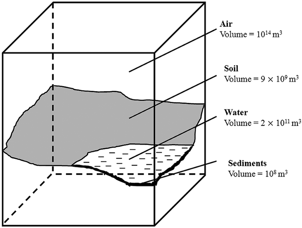 | ||
| Fig. 1 The volumes of the compartments in the evaluated environment. | ||
Modified TOPSIS analysis
TOPSIS was developed by Hwang and Yoon in 1981.35 The general scheme of TOPSIS application can be summarized in a few steps. Firstly, the problem to be solved should be stated. In this case it was the assessment of environmental risk connected with the emission of solvents into the environment or the selection of an environmentally benign one. The next steps are finding the alternatives (here 78 solvents) and criteria (herein, they are described in Table 1) that allow the selection of the best alternative. Then, it is needed to define the preference functions for each of the criteria, usually as “the lower, the better” or “the higher, the better”. Weights are then assigned to set the relative importance of the criteria. This point is usually very tricky, as it is user-dependent and the final ranking strongly depends on the numerical values of the weights (the relative importance of the criteria). Herein, the weights are the result of the Level I multimedia model, and therefore they are not user-dependent and they are methodologically well justified. Then, the TOPSIS algorithm was applied, which is relatively straightforward and may be presented in a few simple eqn (2)–(8) as follows:First, the normalized decision matrix was determined. The normalized value rxy was calculated as follows:
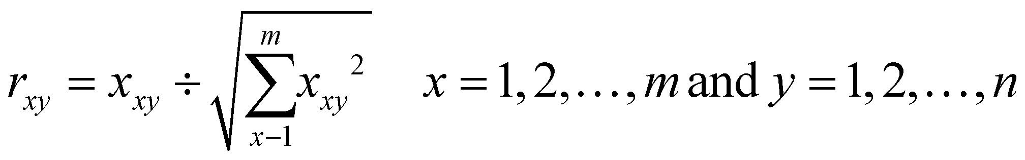 | (2) |
Next, determination of the weighted normalized decision matrix was carried out. The weighted normalized values υxy are calculated as follows:
| υxy = rxy × wxy x = 1, 2, …, m and y = 1, 2, …, n | (3) |
 . In this place, a modification of the original TOPSIS algorithm was introduced. In the original TOPSIS, weights wy are applied to each criterion. The introduced modification to apply different weights wy was methodologically justified, and is described as the “Level I mass balance model” section. The solvent distribution in the environment results from the application of the Level I model. However, the introduced TOPSIS modification requires the preference functions to be none other than “the lower, the better” function.
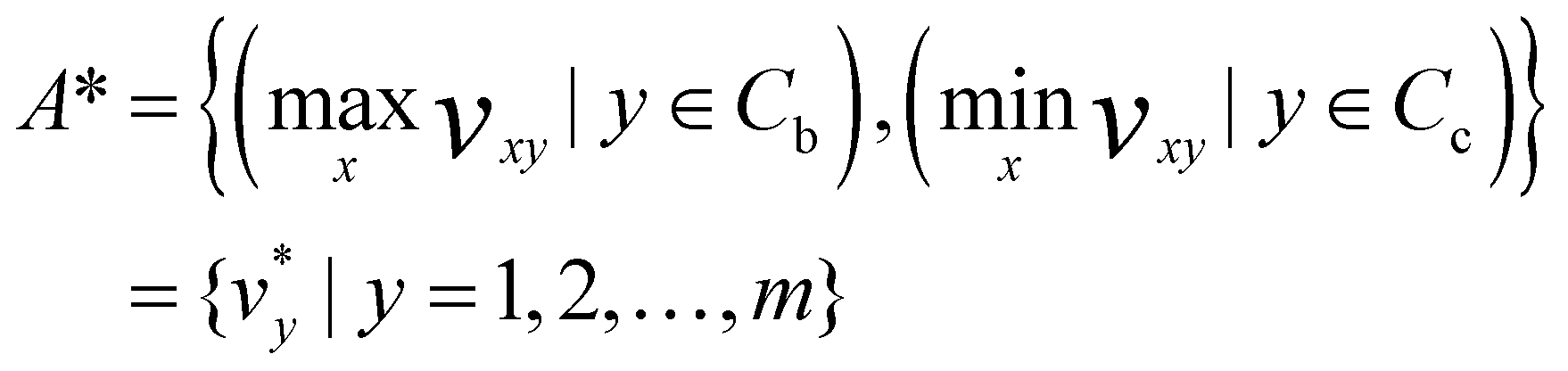
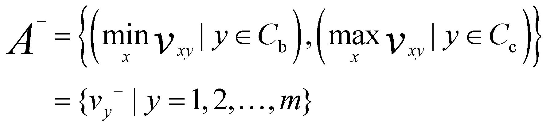
In the next step, determination of the positive ideal solution (A*) and negative ideal solution (A−) was performed.
 | (4) |
Positive ideal solution
 | (5) |
Negative ideal solution
Then, the separation measures using the m-dimensional Euclidean distance were determined. The separation measures of each alternative from the positive ideal solution and the negative ideal solution, respectively, were calculated as follows:
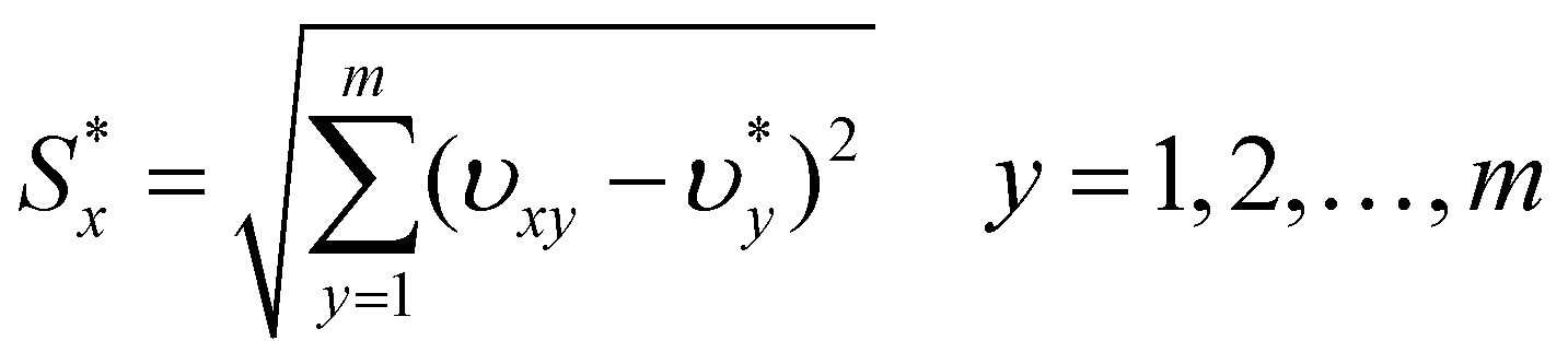 | (6) |
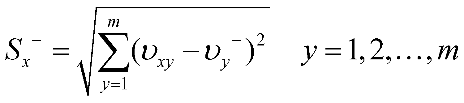 | (7) |
In the last step, determination of the relative closeness to the ideal solution was carried out. The relative closeness of the alternative Ax with respect to A* is defined as follows:
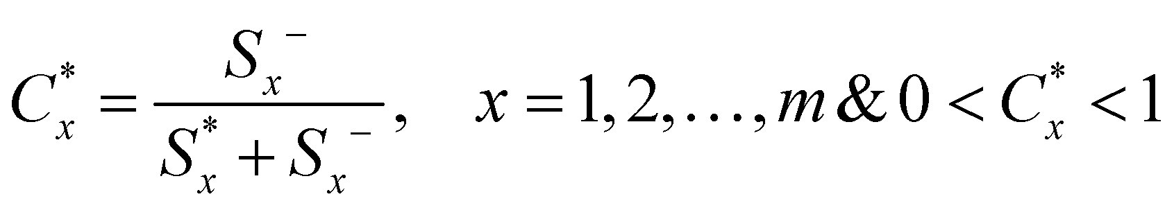 | (8) |
The alternative with  closest to 1 indicates the best preference and can be selected.
Results and discussion
Multimedia model results
The results obtained from applying the Level I model to tert-butyl alcohol, as an example, are presented in Fig. 2. This compound partitions to all four compartments of the evaluative environment, with the majority being present in water (72.5%) and a significant amount is present in air (27.4%). This result appears to be reasonable due to the following reasons: (1) tert-butyl alcohol is polar, and therefore it should be present in water; (2) it is volatile, and hence it is expected to occur in the atmospheric air. An output of the Level I analysis, needed in the further step of the presented approach, is the possible exposure to this chemical in 72.5% coming from the water compartment; 27.4% of the exposure is related to the air compartment and the remaining fraction with the soil and sediment compartments.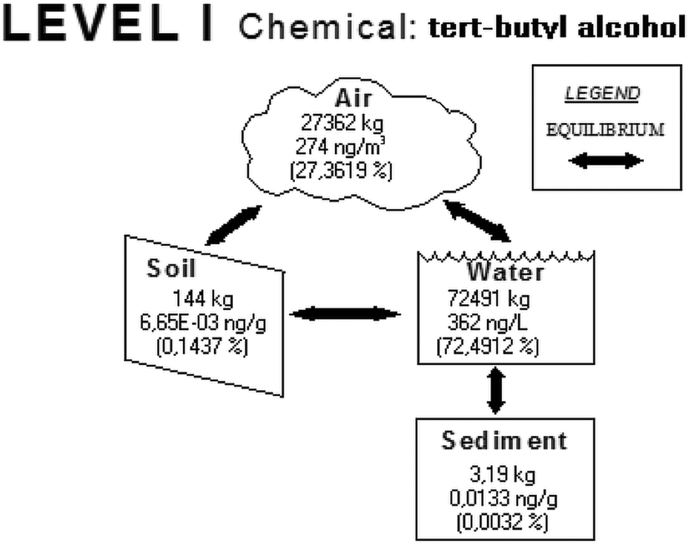 | ||
| Fig. 2 The simplified distribution diagram for tert-butyl alcohol in a four-compartment environment. The amount of emission was assumed to be 100000 kg. | ||
Such results were obtained for all the solvents investigated and are presented in Table 2. According to the model, hydrocarbons partition mainly to air, with the heavier aliphatic ones being present in soil and aromatic ones being noticeable in water and soil. Alcohols are present mainly in water, but a discernible fraction is present in the air and in the soil in case of heavy aliphatic alcohols. Ethers, terpenes and chlorinated solvents are mainly present in the atmospheric air, as are aldehydes; however, in this case a significant fraction partitions to the water compartment. Organic acids and esters partition mainly to water and the environmental behaviour of ketones is variable. Thus it can be concluded that they partition between air and water in the approximate proportion of half by half.
| Group | Solvent | CAS number | Air [%] | Water [%] | Soil [%] | Sediment [%] |
|---|---|---|---|---|---|---|
| Hydrocarbons | Pentane | 109-66-0 | 99.99 | 0.00 | 0.01 | 0.00 |
| Hexane | 110-54-3 | 99.97 | 0.00 | 0.03 | 0.00 | |
| Cyclohexane | 110-82-7 | 99.89 | 0.03 | 0.08 | 0.00 | |
| Heptane | 142-82-5 | 99.95 | 0.00 | 0.05 | 0.00 | |
| Octane | 111-65-9 | 99.73 | 0.00 | 0.26 | 0.01 | |
| Isooctane | 540-84-1 | 99.96 | 0.00 | 0.04 | 0.00 | |
| Nonane | 111-84-2 | 99.61 | 0.00 | 0.38 | 0.01 | |
| Decane | 124-18-5 | 74.11 | 0.03 | 25.30 | 0.56 | |
| Undecane | 1120-21-4 | 73.64 | 0.00 | 25.78 | 0.58 | |
| Dodecane | 112-40-3 | 40.44 | 0.00 | 58.26 | 1.30 | |
| Benzene | 71-43-2 | 98.67 | 0.85 | 0.47 | 0.01 | |
| Toluene | 108-88-3 | 98.99 | 0.74 | 0.26 | 0.01 | |
| o-Xylene | 95-47-6 | 96.99 | 1.37 | 1.60 | 0.04 | |
| m-Xylene | 108-38-3 | 97.72 | 0.94 | 1.31 | 0.03 | |
| p-Xylene | 106-42-3 | 97.97 | 0.91 | 1.10 | 0.02 | |
| Styrene | 100-42-5 | 96.99 | 1.58 | 1.40 | 0.03 | |
| Alcohols | Methanol | 67-56-1 | 9.83 | 90.15 | 0.02 | 0.00 |
| Ethanol | 64-17-5 | 6.59 | 93.37 | 0.04 | 0.00 | |
| 1-Propanol | 71-23-8 | 10.73 | 89.13 | 0.14 | 0.00 | |
| Isopropanol | 67-63-0 | 14.62 | 85.29 | 0.09 | 0.00 | |
| 1-Butanol | 71-36-3 | 15.25 | 84.17 | 0.57 | 0.01 | |
| Isobutanol | 67-63-0 | 46.97 | 52.97 | 0.06 | 0.00 | |
| sec-Butyl alcohol | 78-92-2 | 14.06 | 85.61 | 0.32 | 0.01 | |
| tert-Butyl alcohol | 76-65-0 | 27.36 | 72.49 | 0.14 | 0.01 | |
| 1-Pentanol | 71-41-0 | 20.00 | 77.77 | 2.18 | 0.05 | |
| 1-Hexanol | 111-27-3 | 21.57 | 71.49 | 6.79 | 0.15 | |
| 1-Heptanol | 111-70-6 | 18.65 | 59.80 | 21.08 | 0.47 | |
| 1-Octanol | 111-87-5 | 21.58 | 41.16 | 36.45 | 0.81 | |
| 1-Nonanol | 143-08-8 | 7.67 | 5.28 | 85.15 | 1.90 | |
| Allyl alcohol | 107-18-6 | 9.94 | 89.94 | 0.12 | 0.00 | |
| Benzyl alcohol | 100-51-6 | 0.84 | 98.04 | 1.09 | 0.03 | |
| Glycerol | 56-81-5 | 0.00 | 100.00 | 0.00 | 0.00 | |
| Phenol | 108-95-2 | 2.97 | 94.33 | 2.64 | 0.06 | |
| o-Cresol | 95-45-7 | 4.37 | 88.02 | 7.44 | 0.17 | |
| m-Cresol | 108-39-4 | 2.14 | 90.40 | 7.30 | 0.16 | |
| p-Cresol | 106-44-5 | 2.24 | 90.61 | 6.99 | 0.16 | |
| Ethers | Diethyl ether | 60-29-7 | 93.66 | 6.30 | 0.04 | 0.00 |
| Methyl – tert butyl ether | 1634-04-4 | 91.99 | 7.95 | 0.06 | 0.00 | |
| Furan | 110-00-9 | 99.08 | 0.90 | 0.02 | 0.00 | |
| Tetrahydrofuran | 109-99-9 | 35.83 | 64.00 | 0.17 | 0.00 | |
| Aldehydes | Ethanal | 75-07-0 | 80.53 | 19.42 | 0.05 | 0.00 |
| 1-Propanal | 123-38-6 | 62.18 | 37.69 | 0.13 | 0.00 | |
| 1-Butanal | 123-72-8 | 85.14 | 14.76 | 0.10 | 0.00 | |
| Furfural | 98-08-1 | 6.05 | 93.74 | 0.21 | 0.00 | |
| Ketones | Acetone | 67-64-1 | 61.54 | 38.44 | 0.02 | 0.00 |
| 2-Butanone | 78-93-3 | 42.02 | 57.88 | 0.10 | 0.00 | |
| 2-Pentanone | 107-87-9 | 43.92 | 55.70 | 0.37 | 0.01 | |
| 3-Pentanone | 96-22-0 | 48.84 | 50.79 | 0.36 | 0.01 | |
| Methyl isobutyl ketone | 108-10-1 | 73.06 | 26.37 | 0.56 | 0.01 | |
| 2-Hexanone | 591-78-6 | 37.57 | 61.10 | 1.30 | 0.03 | |
| 2-Heptanone | 110-43-0 | 68.89 | 28.63 | 2.42 | 0.06 | |
| Cyclohexanone | 108-94-1 | 11.89 | 87.60 | 0.50 | 0.01 | |
| Terpenes | D-Limonene | 5989-27-5 | 97.82 | 0.08 | 2.05 | 0.05 |
| p-Cymene | 99-87-6 | 95.41 | 0.44 | 4.06 | 0.09 | |
| α-Pinene | 80-56-8 | 99.31 | 0.03 | 0.65 | 0.01 | |
| β-Pinene | 127-91-3 | 98.25 | 0.08 | 1.63 | 0.04 | |
| Organic acids | Formic acid | 64-18-6 | 0.48 | 99.49 | 0.03 | 0.00 |
| Acetic acid | 64-19-7 | 5.07 | 94.89 | 0.04 | 0.00 | |
| Butyric acid | 107-92-6 | 2.70 | 96.76 | 0.53 | 0.01 | |
| Isobutyric acid | 79-31-2 | 6.21 | 93.05 | 0.72 | 0.02 | |
| Valeric acid | 109-52-4 | 1.65 | 96.21 | 2.09 | 0.05 | |
| Hexanoic acid | 142-62-1 | 0.95 | 92.11 | 6.79 | 0.15 | |
| Esters | Ethyl acetate | 141-78-6 | 73.51 | 26.36 | 0.13 | 0.00 |
| Ethyl acrylate | 140-88-5 | 91.10 | 8.74 | 0.16 | 0.00 | |
| Butyl lactate | 138-22-7 | 1.47 | 97.86 | 0.66 | 0.01 | |
| Ethyl lactate | 97-64-3 | 1.27 | 98.67 | 0.06 | 0.00 | |
| Methyl formate | 107-31-3 | 90.11 | 9.89 | 0.00 | 0.00 | |
| Methyl acetate | 79-20-9 | 88.60 | 11.38 | 0.02 | 0.00 | |
| Methyl laurate | 111-82-0 | 0.00 | 0.36 | 97.48 | 2.16 | |
| Chlorinated | Dichloromethane | 75-09-2 | 97.51 | 2.45 | 0.04 | 0.00 |
| Chloroform | 67-66-3 | 98.66 | 1.25 | 0.09 | 0.00 | |
| Carbon tetrachloride | 56-23-5 | 99.76 | 0.17 | 0.07 | 0.00 | |
| Trichloroethene | 79-01-6 | 99.32 | 0.56 | 0.12 | 0.00 | |
| Tetrachloroethene | 127-18-4 | 99.58 | 0.31 | 0.11 | 0.00 | |
| 1,2-Dichloroethane | 107-06-2 | 96.03 | 3.87 | 0.10 | 0.00 | |
| 1,3-Dichloropropene | 542-75-6 | 97.16 | 2.65 | 0.19 | 0.00 | |
| Hexachlorobutadiene | 87-68-3 | 90.46 | 0.17 | 9.17 | 0.20 | |
| Other | Acetonitrile | 75-05-8 | 41.02 | 58.96 | 0.02 | 0.00 |
Ranking of solvents
Based on the weights (the percentage of distribution) described in Table 2, an environmental risk ranking of the solvents was created using the TOPSIS procedure. By introducing these weights, a very strong relative importance to the hazard criteria was given. As an example, water-related hazards for hexane are ignored as it does not partition to water, and the significant hazards connected with the emission of this compound are related with the air compartment. The full ranking obtained in this way is presented in Table 3.| Rank | Chemical group | Solvent | Molar mass [g] | CAS number | Similarity to ideal solution score |
|---|---|---|---|---|---|
| 1 | Alcohol | 1-Propanol | 60 | 71-23-8 | 0.9545 |
| 2 | Alcohol |

|
46 | 64-17-5 | 0.9300 |
| 3 | Alcohol |

|
74 | 71-36-3 | 0.9213 |
| 4 | Alcohol |

|
74 | 76-65-0 | 0.9183 |
| 5 | Ketone |

|
58 | 67-64-1 | 0.9166 |
| 6 | Organic acid |

|
60 | 64-19-7 | 0.9118 |
| 7 | Organic acid | Formic acid | 46 | 64-18-6 | 0.9118 |
| 8 | Ester |

|
214 | 111-82-0 | 0.9112 |
| 9 | Ester | Methyl formate | 60 | 107-31-3 | 0.9083 |
| 10 | Ester |

|
74 | 79-20-9 | 0.9054 |
| 11 | Hydrocarbon | Dodecane | 170 | 112-40-3 | 0.8919 |
| 12 | Ester |

|
88 | 141-78-6 | 0.8868 |
| 13 | Organic acid | Isobutyric acid | 88 | 79-31-2 | 0.8867 |
| 14 | Alcohol |

|
92 | 56-81-5 | 0.8861 |
| 15 | Ether | Methyl tert-butyl ether | 88 | 1634-04-4 | 0.8855 |
| 16 | Alcohol |

|
88 | 71-41-0 | 0.8836 |
| 17 | Alcohol | Benzyl alcohol | 108 | 100-51-6 | 0.8812 |
| 18 | Alcohol |

|
102 | 111-27-3 | 0.8788 |
| 19 | Ether | Tetrahydrofuran | 72 | 109-99-9 | 0.8779 |
| 20 | Alcohol | 1-Heptanol | 116 | 111-70-6 | 0.8721 |
| 21 | Ketone | 3-Pentanone | 86 | 96-22-0 | 0.8714 |
| 22 | Organic acid | Hexanoic acid | 116 | 142-62-1 | 0.8705 |
| 23 | Hydrocarbon | Decane | 142 | 124-18-5 | 0.8703 |
| 24 | Organic acid | Butyric acid | 88 | 107-92-6 | 0.8702 |
| 25 | Ketone |

|
98 | 108-94-1 | 0.8702 |
| 26 | Organic acid | Valeric acid | 102 | 109-52-4 | 0.8700 |
| 27 | Alcohol |

|
60 | 67-63-0 | 0.8698 |
| 28 | Ester | Butyl lactate | 146 | 138-22-7 | 0.8697 |
| 29 | Ester |

|
188 | 97-64-3 | 0.8694 |
| 30 | Alcohol | 1-Octanol | 130 | 111-87-5 | 0.8689 |
| 31 | Other |

|
41 | 75-05-8 | 0.8687 |
| 32 | Hydrocarbon | Undecane | 156 | 1120-21-4 | 0.8677 |
| 33 | Alcohol |

|
32 | 67-56-1 | 0.8644 |
| 34 | Aldehyde | 1-Propanal | 58 | 123-38-6 | 0.8636 |
| 35 | Aldehyde | 1-Butanal | 72 | 123-72-8 | 0.8608 |
| 36 | Aldehyde |

|
96 | 98-08-1 | 0.8586 |
| 37 | Alcohol | 1-Nonanol | 144 | 143-08-8 | 0.8583 |
| 38 | Alcohol |

|
74 | 67-63-0 | 0.8525 |
| 39 | Hydrocarbon | Pentane | 72 | 109-66-0 | 0.8475 |
| 40 | Ketone | 2-Hexanone | 100 | 591-78-6 | 0.8456 |
| 41 | Hydrocarbon | Nonane | 128 | 111-84-2 | 0.8427 |
| 42 | Ketone | 2-Heptanone | 114 | 110-43-0 | 0.8400 |
| 43 | Hydrocarbon | Isooctane | 114 | 540-84-1 | 0.8342 |
| 44 | Hydrocarbon | Octane | 114 | 111-65-9 | 0.8330 |
| 45 | Alcohol | sec-Butyl alcohol | 74 | 78-92-2 | 0.8285 |
| 46 | Ketone |

|
72 | 78-93-3 | 0.8208 |
| 47 | Ether | Diethyl ether | 74 | 60-29-7 | 0.8168 |
| 48 | Alcohol | p-Cresol | 108 | 106-44-5 | 0.8090 |
| 49 | Alcohol | o-Cresol | 108 | 95-45-7 | 0.8081 |
| 50 | Alcohol | Allyl alcohol | 58 | 107-18-6 | 0.8073 |
| 51 | Hydrocarbon | Heptane | 100 | 142-82-5 | 0.8021 |
| 52 | Hydrocarbon | Cyclohexane | 84 | 110-82-7 | 0.7892 |
| 53 | Terpene |

|
136 | 127-91-3 | 0.7815 |
| 54 | Alcohol | Phenol | 94 | 108-95-2 | 0.7789 |
| 55 | Hydrocarbon | m-Xylene | 106 | 108-38-3 | 0.7594 |
| 56 | Alcohol | m-Cresol | 108 | 108-39-4 | 0.7558 |
| 57 | Terpene |

|
136 | 80-56-8 | 0.7475 |
| 58 | Ketone | 2-Pentanone | 86 | 107-87-9 | 0.7362 |
| 59 | Hydrocarbon | Toluene | 92 | 108-88-3 | 0.7344 |
| 60 | Terpene |

|
134 | 99-87-6 | 0.7252 |
| 61 | Chlorinated | Dichloromethane | 85 | 75-09-2 | 0.7150 |
| 62 | Hydrocarbon | p-Xylene | 106 | 106-42-3 | 0.7072 |
| 63 | Hydrocarbon | Hexane | 86 | 110-54-3 | 0.7057 |
| 64 | Chlorinated | 1,2-Dichloroethane | 99 | 107-06-2 | 0.6954 |
| 65 | Ketone |

|
100 | 108-10-1 | 0.6939 |
| 66 | Chlorinated | 1,3-Dichloropropene | 111 | 542-75-6 | 0.6922 |
| 67 | Chlorinated | Dichloroform | 119 | 67-66-3 | 0.6862 |
| 68 | Chlorinated | Tetrachloroethene | 166 | 127-18-4 | 0.6841 |
| 69 | Ester | Ethyl acrylate | 100 | 140-88-5 | 0.6787 |
| 70 | Hydrocarbon | Styrene | 104 | 100-42-5 | 0.6786 |
| 71 | Hydrocarbon | o-Xylene | 106 | 95-47-6 | 0.6715 |
| 72 | Terpene |

|
136 | 5989-27-5 | 0.6641 |
| 73 | Aldehyde | Ethanal | 44 | 75-07-0 | 0.6572 |
| 74 | Chlorinated | Carbon tetrachloride | 154 | 56-23-5 | 0.6424 |
| 75 | Chlorinated | Trichloroethene | 131 | 79-01-6 | 0.6291 |
| 76 | Hydrocarbon | Benzene | 78 | 71-43-2 | 0.6098 |
| 77 | Ether | Furan | 68 | 110-00-9 | 0.4755 |
| 78 | Chlorinated | Hexachlorobutadiene | 261 | 87-68-3 | 0.4044 |
Some of the solvents present in the ranking are recognised as green in numerous references. Those solvents that have been reported as being green are highlighted in grey in Table 3.36,37 Remarkably, 1-propanol was ranked first even though it has not been considered as a green solvent, presumably due to its high impact during the stage of petrochemical production.38 The results of this study show that 1-propanol can be considered as a green solvent concerning its environmental risks after emission. Thus, finding more sustainable synthetic pathways for the production of 1-propanol would make this solvent ideal as a replacement for conventional hazardous solvents. The second most preferable organic solvent was ethanol, being assessed as a green solvent by the pharmaceutical solvent selection guides.39 Ethanol partitions mainly to water, and therefore the hazards related to this environmental compartment are relevant in its case. It has a very low logBCF, it is non-toxic to fish and is readily biodegradable. It has been used as a green alternative in extraction processes40 and as a mobile phase in liquid chromatography.41 The third rank was gained by 1-butanol, another green, acceptable solvent. The fourth rank was obtained by tert-butyl alcohol, a solvent widely accepted as green. It was ranked lower than ethanol because of its higher toxicity towards fish and higher inhalation toxicity; in the case of this solvent, the partitioning to air compartment plays a more important role (27.4%) when compared to ethanol (6.6%). Acetone, placed at five in the ranking, is referred as a green alternative, along with ethanol, and is used as a green mobile phase constituent in liquid chromatography.42 The next two ranking locations are scored by acetic and formic acids. Their parameters do not differ much since formic acid is more toxic, but more readily biodegradable and is characterized by a lower POCP. Acetic acid and formic acid are ranked high as relatively green solvents. The pharmaceutical solvent selection guide states that the utilization of these solvents was acceptable in terms of their environmental aspects.39 However, their poor assessment score in the “health” criteria makes their overall score as “problematic”.
Another solvent widely recognized as green is glycerol. It is obtained from plant oils with its price depending on the purity grade and is considered to be a renewable resource.43 In fact, it is a by-product of biodiesel production from triglycerides as a raw material,44 but this process yield is not high. It possesses a series of desired properties as a solvent and its main drawback is its high viscosity.45 It is relatively non-toxic via oral exposure.46 Application of Level I fugacity model shows that it partitions to water only. The important factors are toxicity towards fish, bioconcentration factor, biodegradability and oral LD50. For all of these criteria, glycerol performs well even though there are solvents that are characterized with better values for all of the assessment criteria. This is the reason for glycerol being present at the 14th position in the ranking among other green solvents.
In general terms, methyl and ethyl esters are ranked high. They undergo fast biodegradation, do not undergo bioconcentration, and show low or moderate toxicity towards fish and rodents when administered orally or via inhalation. However, ethyl acrylate (rank 69) is marked as a potential carcinogen. It is also characterized by a relatively high inhalation toxicity. Ethyl lactate (rank 29) was investigated in more detail as a potential green solvent due to its favourable properties, apart from previously mentioned ones, such as low price and being approved to be used in food products.47 The application of this solvent in industry can be challenging due to its high viscosity and resulting poor mass transfer parameters.48
A very interesting result is the low position of all terpenes in the rankings. β-Pinene, α-pinene, p-cymene and D-limonene are ranked 53, 57, 60 and 72, respectively. The results of the Level I model show that terpenes partition mainly to atmospheric air. Their POCP values are particularly high and their inhalation toxicities are at moderate levels. The POCP value for D-limonene even defines the anti-ideal solution; it indicates that it is the highest in the entire dataset. However, terpenes are considered to be green solvents as stated in numerous reports and there is reasoning behind this statement. For example, D-limonene can be obtained from citrus oils, and therefore it is a bio-based solvent, obtained often from food industry waste, and it is biodegradable.49 It is characterized by low oral toxicity and it performs well when it substitutes traditionally used organic solvents such as hexane50 or toluene.51 Similarly, α-pinene is a solvent obtained from a bio-based and renewable resource, conifer waste.52 The results of the present study show that the environmental risk associated with the emission of terpenes is considerable in relation to the other solvents, and thus it has to be taken into consideration when selecting terpenes as the solvent in various processes.
Solvents that are carcinogens, potential or possible carcinogens, toxic or causing other effects are located in the lower part of the ranking. Without any discussion, hexachlorobutadiene, trichloroethene and other chlorinated solvents, benzene, styrene and xylenes have to be treated as undesirable solvents.
It is worth noting that the present assessment methodology does not include the data used for full LCA methodology, does not include safety data and partially covers health data used in EHS based approach. Despite these facts, the obtained results are generally in good agreement with the results reported by other solvent assessment tools.37 Some deviations are related to the environmental risk assessment of terpenes, although these discrepancies are methodologically well justified by our approach.
As our assessment methodology does not include any information that influences the sustainability of solvents during pre-emission stages, application of an additional assessment tool is required. It might be detailed in the LCA that includes origin of feedstock used to solvent production, manufacturing purposes and safety issues in assessment protocol.
Conclusions
The presented study provides a novel approach to assess the environmental risk related to solvent emissions. The results of Level I modelling give an overview of solvent distribution in the environmental compartments and can be used at the initial stage of solvent assessment. This model also supplies methodologically justified weights to the MCDA. Ranking with the MCDA analysis results shows the relative environmental risks of the emitted solvents. The least environmentally problematic are short chain alcohols, esters, and some carboxylic acids. The solvents that pose some serious threats to the environment are chlorinated solvents, aromatic hydrocarbons and, quite surprisingly, terpenes.The proposed assessment procedure can give some other results if a different evaluative environment is considered. The proposed approach may be applied for case studies, when solvents are selected for application in specific locations. To fit the case study, different criteria reflecting the hazards can be applied as input data in the assessment procedure and different results can be obtained.
The assessment procedure is focused on the environmental risks related to solvent emissions. Therefore, this tool is favourable when the application of the solvent is related to its release to the environment. On the other hand, as only the environmental aspect is considered, the procedure can be treated as a screening tool and when used for full assessment it has to be supported by LCA.
Acknowledgements
F. Pena-Pereira thanks Xunta de Galicia for financial support as a post-doctoral researcher of the I2C program.References
- P. T. Anastas and J. Warner, Green Chemistry Theory and practice, Oxford University Press, Oxford, 1998 Search PubMed.
- M. Poliakoff, J. M. Fitzpatrick, T. R. Farren and P. T. Anastas, Science, 2002, 297, 807–810 CrossRef CAS PubMed.
- R. K. Henderson, C. Jimenez-Gonzalez, D. J. C. Constable, S. R. Alston, G. G. A. Inglis, G. Fisher, J. Sherwood, S. P. Binks and A. D. Curzons, Green Chem., 2011, 13, 854–862 RSC.
- D. Prat, O. Pardigon, H.-W. Flemming, S. Letestu, V. Ducandas, P. Isnard, E. Guntrum, T. Senac, S. Ruisseau, P. Cruciani and P. Hosek, Org. Process Res. Dev., 2013, 17, 1517–1525 CrossRef CAS.
- K. K. Alfonsi, J. Colberg, P. J. Dunn, T. Fevig, S. Jennings, T. A. Johnson, H. P. Kleine, C. Knight, M. A. Nagy, D. A. Perry and M. Stefaniak, Green Chem., 2008, 10, 31–36 RSC.
- S. Hellweg, U. Fischer, M. Scheringer and K. Hungerbühler, Green Chem., 2004, 6, 418–427 RSC.
- A. Amelio, G. Genduso, S. Vreysen, P. Luis and B. Van der Bruggen, Green Chem., 2014, 16, 3045–3063 RSC.
- C. Capello, U. Fischer and K. Hungerbühler, Green Chem., 2007, 9, 927–934 RSC.
- I. B. Huang, J. Keisler and I. Linkov, Sci. Total Environ., 2011, 409, 3578–3594 CrossRef CAS PubMed.
- M. Tobiszewski and A. Orłowski, J. Chromatogr., A, 2015, 1387, 116–122 CrossRef CAS PubMed.
- D. Kralisch, C. Staffel, D. Ott, S. Bensaid, G. Saracco, P. Bellantoni and P. Loeb, Green Chem., 2013, 15, 463–477 RSC.
- P. Gramatica, S. Cassani and A. Sangion, Green Chem., 2016, 18, 4393–4406 RSC.
- P.-M. Jacob, P. Yamin, C. Perez-Storey, M. Hopgood and A. A. Lapkin, Green Chem. 10.1039/c6gc02482c.
- M. Behzadian, S. K. Otaghsara, M. Yazdani and J. Ignatius, Expert Syst. Appl., 2012, 39, 13051–13069 CrossRef.
- G. Sakthivel, M. Ilangkumaran and A. Gaikwad, Ain Shams Eng. J., 2015, 6, 239–256 CrossRef.
- H. Al-Hazmi, J. Namieśnik and M. Tobiszewski, Curr. Anal. Chem., 2016, 12, 261–267 CrossRef CAS.
- P. Bigus, J. Namieśnik and M. Tobiszewski, J. Chromatogr., A, 2016, 1446, 21–26 CrossRef CAS PubMed.
- D. Mackay and S. Paterson, Environ. Sci. Technol., 1982, 16, 654A–660A CAS.
- D. Mackay, Multimedia Environmental Models The Fugacity Approach, CRC Press LLC, USA, 2001 Search PubMed.
- D. Mackay, A. Di Guardo, S. Paterson and C. E. Cowan, Environ. Toxicol. Chem., 1996, 15, 1627–1637 CrossRef CAS.
- D. Mackay, A. Di Guardo, S. Paterson, G. Kicsi, C. E. Cowan and D. M. Kane, Environ. Toxicol. Chem., 1996, 15, 1638–1648 CrossRef CAS.
- S. Gama, D. Mackay and J. A. Arnot, Green Chem., 2012, 14, 1094–1102 RSC.
- M. Tobiszewski, S. Tsakovski, V. Simeonov, J. Namieśnik and F. Pena-Pereira, Green Chem., 2015, 17, 4773–4785 RSC.
- D. Mackay, W. Y. Shiu, K.-C. Ma and S. C. Lee, Handbook of Physical-Chemical Properties and Environmental Fate for Organic Chemicals, Taylor & Francis, Boca Raton, USA, 2006 Search PubMed.
- Y. Andersson-Sköld, P. Grennfelt and K. Pleijel, J. Air Waste Manage. Assoc., 1992, 42, 1152–1158 Search PubMed.
- W. Wu, B. Zhao, S. Wang and J. Hao, J. Environ. Sci. DOI:10.1016/j.jes.2016.03.025.
- J. Altenstedt and K. Pleijel, J. Air Waste Manage. Assoc., 2000, 50, 1023–1036 CAS.
- International Agency for Cancer Research, website http://www.iarc.fr (visited 27.09.2016).
- C. M. Alder, J. D. Hayler, R. K. Henderson, A. M. Redman, L. Shukla, L. E. Shuster and H. F. Sneddon, Green Chem., 2016, 18, 3879–3890 RSC.
- E. Calabrese, R. Barnes and E. J. Stanek, Regul. Toxicol. Pharmacol., 1989, 10, 123–137 CrossRef CAS PubMed.
- The Canadian Centre for Environmental Modelling and Chemistry Level I Model Version 2.11 - August 1999. http://www.trentu.ca/academic/aminss/envmodel/models/VBL1.html (visited 27.09.2016).
- D. Mackay, A. Di Guardo, S. Paterson and C. E. Cowan, Environ. Toxicol. Chem., 1996, 15, 1627–1637 CrossRef CAS.
- W.-H. Chen, W.-B. Yang, C.-S. Yuan, J.-C. Yang and Q.-L. Zhao, Chemosphere, 2014, 103, 92–98 CrossRef CAS PubMed.
- C. Fan, Y.-c. Chen, H.-w. Ma and G.-s. Wang, J. Hazard. Mater., 2010, 182, 778–786 CrossRef CAS PubMed.
- C. L. Hwang and K. P. Yoon, Multiple attribute decision making: Methods and applications, Springer-Verlag, Ney York, 1981 Search PubMed.
- D. Prat, A. Wells, J. Hayler, H. Sneddon, C. R. McElroy, S. Abou-Shehada and P. J. Dunn, Green Chem., 2016, 18, 288–296 RSC.
- F. P. Byrne, S. Jin, G. Paggiola, T. H. M. Petchey, J. H. Clark, T. J. Farmer, A. J. Hunt, C. R. McElroy and J. Sherwood, Sustainable Chem. Processes, 2016, 4, 1–24 CrossRef.
- C. Capello, U. Fischer and K. Hungerbühler, Green Chem., 2007, 9, 927–934 RSC.
- D. Prat, J. Hayler and A. Wells, Green Chem., 2014, 16, 4546–4551 RSC.
- R. Cardoso de Oliveira, S. T. Davantel de Barros and M. Luiz Gimenes, J. Food Eng., 2013, 117, 458–463 CrossRef.
- Y. Shen, B. Chen and T. A. van Beek, Green Chem., 2015, 17, 4073–4081 RSC.
- C. S. Funari, R. L. Carneiro, M. M. Khandagale, A. J. Cavalheiro and E. F. Hilder, J. Sep. Sci., 2015, 38, 1458–1465 CrossRef CAS PubMed.
- Y. Gu and F. Jérôme, Green Chem., 2010, 12, 1127–1138 RSC.
- A. E. Díaz-Álvarez, J. Francos, P. Crochet and V. Cadierno, Curr. Green Chem., 2014, 1, 51–65 CrossRef.
- J. I. García, H. García-Marín and E. Pires, Green Chem., 2014, 16, 1007–1033 RSC.
- A. Wolfson, C. Dlugy and Y. Shotland, Environ. Chem. Lett., 2007, 5, 67–71 CrossRef CAS.
- S. Aparicio and R. Alcalde, Green Chem., 2009, 11, 65–78 RSC.
- Y. L. Kua, S. Gan, A. Morris and H. K. Ng, Sustainable Chem. Pharm., 2016, 4, 21–31 CrossRef.
- Y. Zhu, Z. Chen, Y. Yang, P. Cai, J. Chen, Y. Li, W. Yang, J. Peng and Y. Cao, Org. Electron., 2015, 23, 193–198 CrossRef CAS.
- M. Virot, V. Tomao, C. Ginies, F. Visinoni and F. Chemat, J. Chromatogr., A, 2008, 1196–1197, 147–152 CrossRef CAS PubMed.
- S. Veillet, V. Tomao, K. Ruiz and F. Chemat, Anal. Chim. Acta, 2010, 674, 49–52 CrossRef CAS PubMed.
- S. Bertouche, V. Tomao, K. Ruiz, A. Hellal, C. Boutekedjiret and F. Chemat, Food Chem., 2012, 134, 602–605 CrossRef CAS.
Footnote |
| † Electronic supplementary information (ESI) available. See DOI: 10.1039/c6gc03424a |
| This journal is © The Royal Society of Chemistry 2017 |