A fully general time-dependent multiconfiguration self-consistent-field method for the electron–nuclear dynamics
Received
31st March 2017
, Accepted 25th July 2017
First published on 25th July 2017
Abstract
We present a fully general time-dependent multiconfiguration self-consistent-field method to describe the dynamics of a system consisting of arbitrarily different kinds and numbers of interacting fermions and bosons. The total wave function is expressed as a superposition of different configurations constructed from time-dependent spin-orbitals prepared for each particle kind. We derive equations of motion followed by configuration–interaction (CI) coefficients and spin-orbitals for general, not restricted to full-CI, configuration spaces. The present method provides a flexible framework for the first-principles theoretical study of, e.g., correlated multielectron and multinucleus quantum dynamics in general molecules induced by intense laser fields and attosecond light pulses.
1 Introduction
We are now witnessing rapid progress in ultrashort intense light sources in different spectral ranges such as terahertz radiation, optical-parametric-chirped-pulse-amplification mid-infrared lasers, high-harmonic extreme-ultraviolet (XUV) pulses, and XUV/X-ray free-electron lasers. These technological advances have triggered various research activities, including attosecond science,1–3 with a goal to directly measure and, ultimately, control electron and nuclear motion in atoms and molecules.
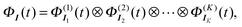
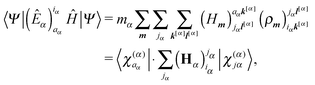
Ab initio simulations of the electronic and nuclear dynamics in atoms and molecules remain a challenge. A multiconfiguration time-dependent Hartree–Fock (MCTDHF) method4,5 has been developed for the investigation of multielectron dynamics in strong and/or ultrashort laser fields.6 In this approach, the time-dependent total electronic wave function Ψ(t) is expressed as a superposition of different Slater determinants ΦI(t),
| |  | (1) |
where
CI(
t) is the configuration–interaction (CI) coefficients. Both {
CI(
t)} and the spin-orbitals constituting {
ΦI(
t)} are allowed to vary in time. In the community of high-field phenomena and attosecond physics, the term MCTDHF is conventionally used for the full-CI case, in which the sum in
eqn (1) runs over all the possible ways to distribute the electrons among a given number of spin-orbitals. On the other hand, also under active development are variants without the restriction to the full-CI expansion, generically referred to as the time-dependent multiconfiguration self-consistent-field (TD-MCSCF) methods hereafter. Representative examples include the time-dependent complete-active-space self-consistent-field,
7,8 the time-dependent restricted-active-space self-consistent-field,
9 and the time-dependent occupation-restricted multiple active-space (TD-ORMAS)
10 methods. These allow a compact and computationally less demanding description of the multielectron dynamics, without sacrificing the accuracy. In particular, the TD-ORMAS method can treat arbitrary CI expansions of the form
eqn (1) in principle.
Among successful approaches for nuclear dynamics is the multiconfiguration time-dependent Hartree (MCTDH) method.11 Developed for systems consisting of distinguishable particles, this method expresses the time-dependent total nuclear wave function as a superposition similar to eqn (1) but that of Hartree products. The other way around, the MCTDHF method can be viewed as an extension of the MCTDH method to fermions. By hybridizing the MCTDHF method for electrons and the MCTDH method for nuclei, one can construct a multiconfiguration electron–nuclear dynamics (MCEND) method12,13 to describe the non-Born–Oppenheimer coupled dynamics. Nuclei forming molecules are, however, indistinguishable particles, either fermions or bosons. Alon et al. have explored methods for systems consisting of identical particles,14–17e.g., MCTDH methods for mixtures consisting of two14 and three17 kinds of identical particles, and inclusion of particle conversion.16 Kato and Yamanouchi have extended the MCTDHF theory to molecules composed of electrons, (fermionic) protons, and two heavy (either classical or quantum) nuclei.18
In this paper, further stepping forward in this direction, we present a fully general TD-MCSCF method for a system comprising arbitrarily different kinds and numbers of interacting fermions and bosons (without particle conversion16). Treating all the constituent particles on an equal footing, we expand the total wave function in terms of configurations of the whole system [see eqn (5) below]. Thus, based on the time-dependent variational principle, we derive the equations of motion (EOM) of CI coefficients and spin-orbitals for general configuration spaces, not restricted to full-CI. As a simple example, we apply the TD-MCSCF method to high-harmonic generation (HHG) from a one-dimensional (1D) model hydrogen molecular ion H2+ induced by an intense near-infrared (NIR) laser pulse, for which numerically exact solution is available.
This paper is organized as follows. Section 2 introduces our TD-MCSCF ansatz for many-particle systems composed of different kinds of fermions and bosons, and also defines the target Hamiltonian considered in this work. In Section 3, we derive the general equations of motion, based on the time-dependent variational principle. Explicit working equations for a molecule interacting with an external laser field are shown in Section 4. We present numerical examples in Section 5. Concluding remarks are given in Section 6.
2 Definition of the problem
2.1 TD-MCSCF ansatz
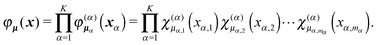
We consider a quantum mechanical many-body system with K kinds of fermions or bosons. The subsystem of kind α consists of Nα identical particles. Thus, there are  particles as a whole. For notational brevity, we call such a system an N-particle system, where the array of integers N = (N1N2⋯NK) carries the information of both particle kinds and the number of particles in each kind.
Let us define, for each kind of particles, the complete orthonormal set of spin-orbitals  , which spans the one-particle Hilbert space Ωα, is time-dependent in general. Then the N-particle Hilbert space is spanned by
| |  | (2) |
where

is a determinant (or permanent) of
α-kind fermions (or bosons), consisting of
Nα spin-orbitals chosen from

. We call
ΦI(
t) the
I’s configuration, where
I =
I1I2⋯
IK is considered, at the moment, to collectively label the chosen spin-orbitals. The objective of this paper is to formulate the TD-MCSCF theory of the
N-particle system within the ansatz of total wavefunction analogous to that for the electronic system,
eqn (1), but using the configurations of
eqn (2).
For rigorous and compact presentation of theory, we resort to the second quantization formulation by introducing creation and annihilation operators  associated with
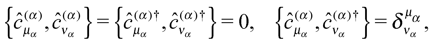
  . These operators obey the (anti-)commutation relations of bosons (fermions),
| |  | (3) |
for bosons, where [
â,
![[b with combining circumflex]](https://www.rsc.org/images/entities/i_char_0062_0302.gif)
] =
â −
â, and
| |  | (4) |
for fermions, where {
â,
} =
â +
â.
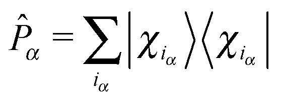
Within the TD-MCSCF ansatz, the complete set of spin-orbitals  is split into nα (≥Nα for fermions) occupied spin-orbitals
  and remaining virtual spin-orbitals
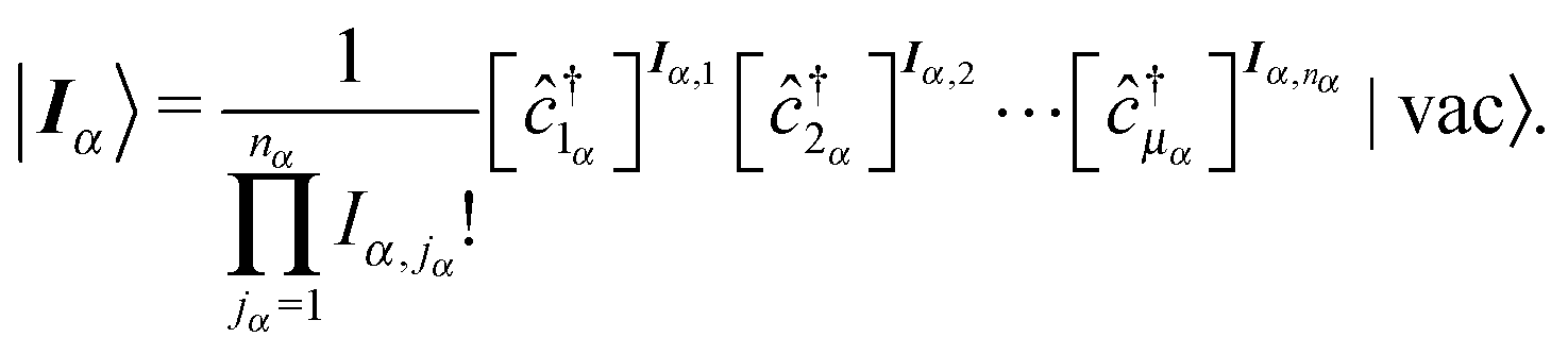
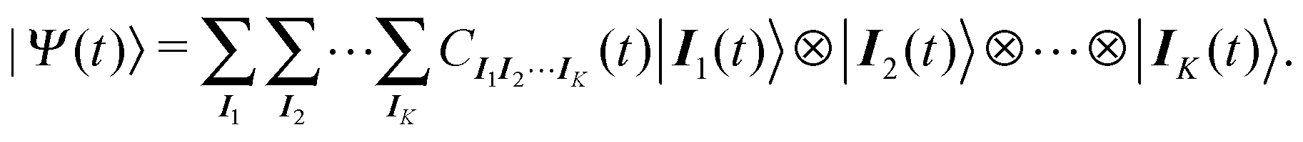
  . We call the subspace of Ωα spanned by occupied spin-orbitals the occupied spin-orbital space Ωoccα, and that spanned by virtual spin-orbitals the virtual spin-orbital space Ωvirα, where Ωα = Ωoccα ⊕ Ωvirα. The total state Ψ(t) is expressed as a superposition of configurations ΦI(t) of eqn (2), but constructed from occupied spin-orbitals only. Thus we write
| |  | (5) |
where
CI(
t) is the CI coefficient, and |
I(
t)〉 is the occupation number representation of the configuration
ΦI,
| | | |I(t)〉 = |I1(t)〉 ⊗ |I2(t)〉 ⊗⋯⊗ |IK(t)〉, | (6) |
| |  | (7) |
Now
Iα =
Iα,1Iα,2⋯
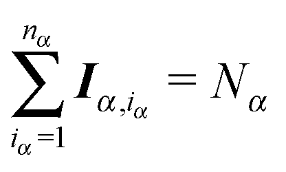
Iα,nα is (rigorously) reinterpreted as an integer array, satisfying

. Note that
Iα,iα ∈ {0,1} for fermions. Here and in what follows, we use indices
iα,
jα,
kα,… for occupied (
Ωoccα),
aα,
bα,
cα,… for virtual (
Ωvirα), and
μα,
να,
κα,
τα,… for general (
Ωα) spin-orbitals of kind
α. The indices
pα,
qα will be used for numbering the coordinates.
It should be noted that we do not restrict the expansion eqn (5) to the full-CI one. It should also be noticed that occupied configurations are specified in terms of the whole system rather than in terms of each particle kind as,17
| |  | (8) |
with summation over
I1,
I2,…,
IK taken independently.
Eqn (8) implies that given the set of configurations {
Iα} for each kind, the set of configurations for the whole system {
I} must include all the direct products of {{
Iα};
α = 1, 2,…,
K}. Our approach based on
eqn (5), including
eqn (8) as a special case, allows a highly flexible choice of CI space,
e.g., including up to double excitations,
10 regardless of particle kind, from a reference configuration of the whole system, thereby enabling a proper account of correlation between different kinds of particles while reducing the computational cost.
2.2 Target Hamiltonian
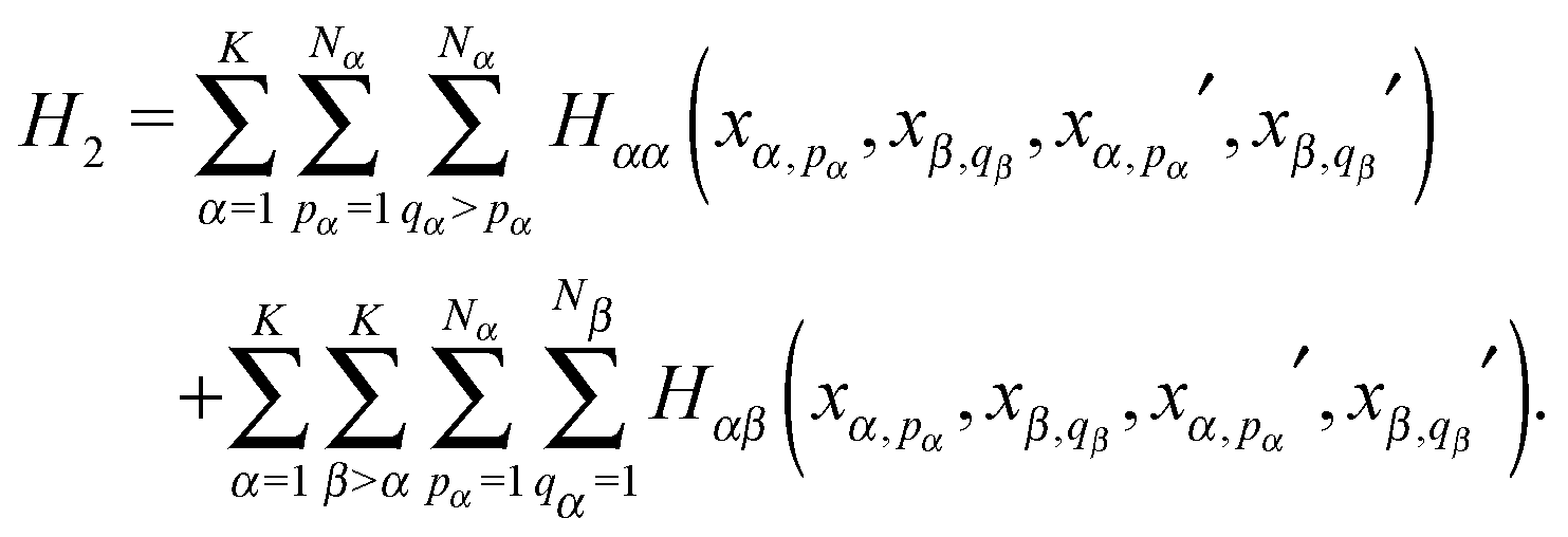
In this article, we consider the Hamiltonian of an N-particle system composed of up to M-body terms,| | | H = H1 + H2 +⋯+ HM, M ≤ N. | (9) |
The Hamiltonian is explicitly time-dependent in general, but the time argument t is dropped in this section for simplicity. Here, the m-body Hamiltonian is assumed to be given explicitly in terms of the coordinates (and momenta, see below) in a general sense characterizing m particles (or degrees of freedom), and symmetric under exchange of coordinates among particles of the same kind. One-particle Hamiltonian, e.g., is written as| |  | (10) |
where the non-local form allows us to describe the momentum dependence of the Hamiltonian, and two-body interaction is generally given by16| | 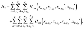 | (11) |
The reasons why we here consider the (non-local) higher-than-two body terms, which will not actually be used in Section 4, are (1) that such a form is used in the multiconfiguration Hartree (MCH) method for distinguishable particles, and (2) their possible appearance upon coordinate transformations, or in the effort of removing translational and rotational degrees of freedom.19,20
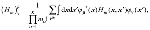
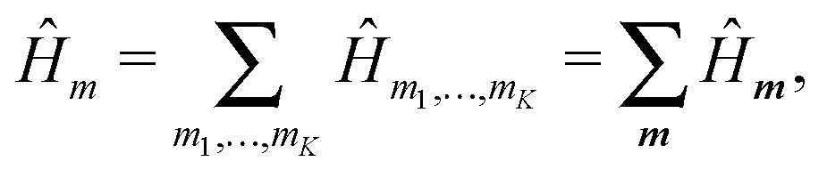
The Hamiltonian is equivalently expressed in the second quantization formalism as
| | 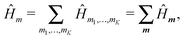 | (12) |
where the net
m-body Hamiltonian is further classified into those contributions
Ĥm, hereafter called the
m-body Hamiltonian, involving
mα particles of the kind
α, (0 ≤
mα ≤
Nα,

),
| | 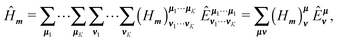 | (13) |
where
μ = (
μ1μ2⋯
μK), and
μα = (
μα,1μα,2⋯
μα,mα) indexes the set of spin-orbitals to represent
mα particles in the Hamiltonian.
Êμν is the
m-particle replacement operator
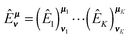
, with
| |  | (14) |
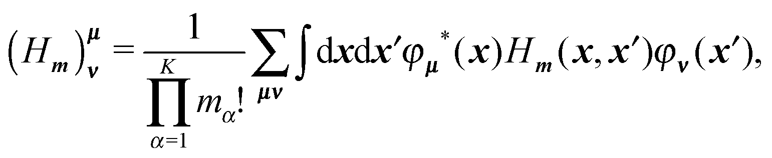
and (
Hm)
mν is given by
| |  | (15) |
where
x = (
x1x2,…,
xK),
xα = (
xα,1xα,2⋯
xα,mα) is the set of
mα coordinates of particle
α, and
| |  | (16) |
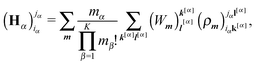
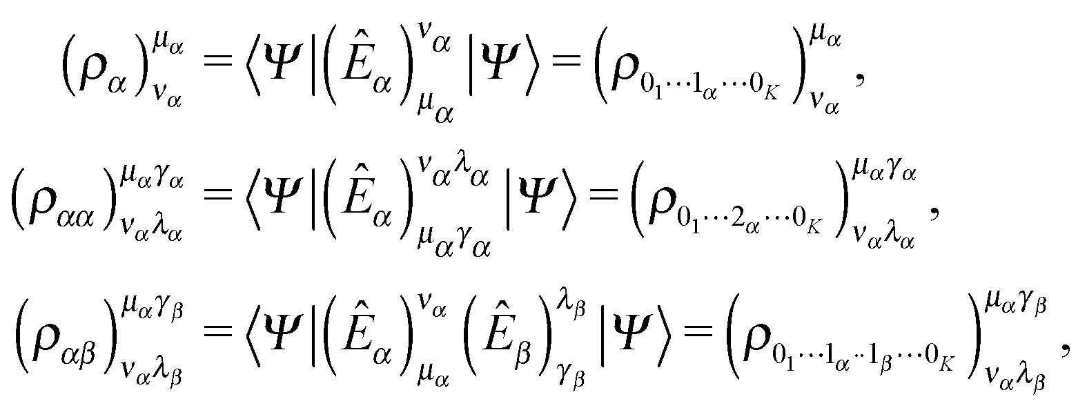
For the later discussion, we define the
m-body reduced density matrix (RDM) as
One- and two-particle RDMs are also denoted as
| |  | (18) |
with
β ≠
α.
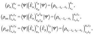
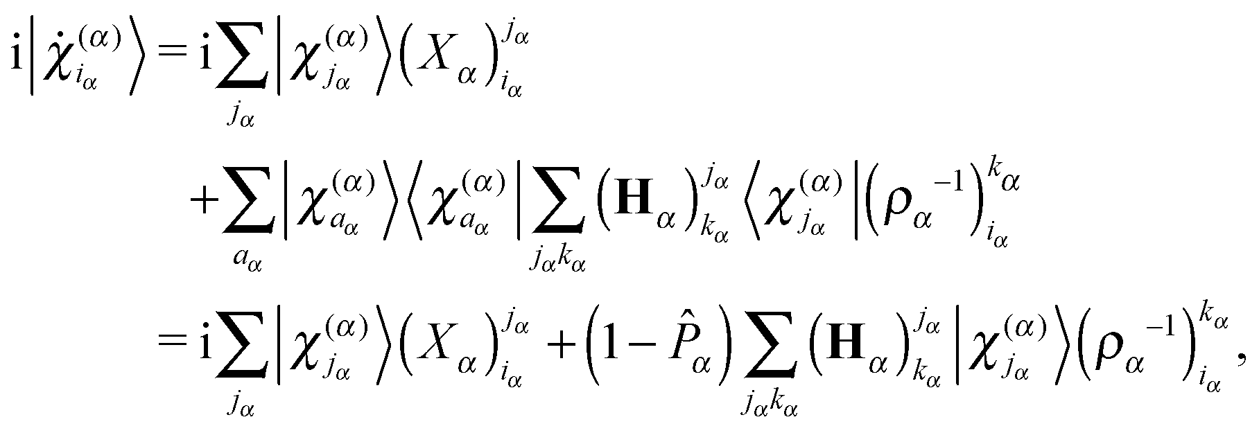
3 Equations of motion
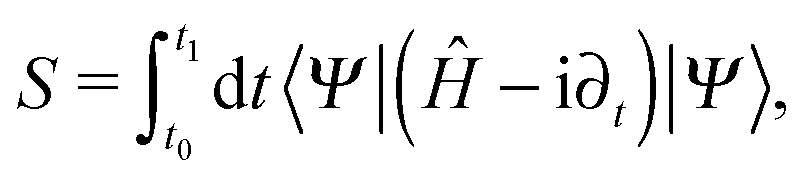
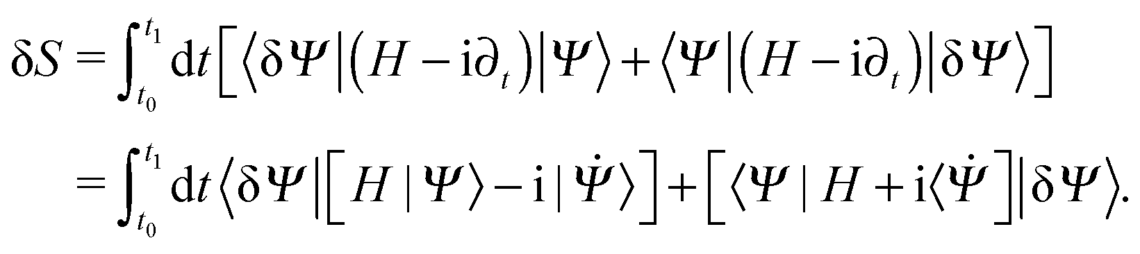
In this section, we derive the EOMs for the CI coefficients and spin-orbitals by imposing the time-dependent variational principle21–23 on our TD-MCSCF ansatz. We require the action integral| |  | (19) |
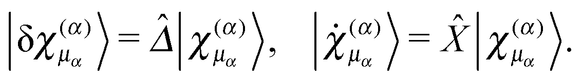
to be stationary, δS = 0, with respect to the variation of the total wavefunction δΨ within our TD-MCSCF ansatz eqn (5), subject to the boundary conditions δΨ(t0) = δΨ(t1) = 0. To this end, let us introduce anti-Hermitian matrices Δα and Xα as,| | 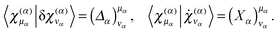 | (20) |
(Recall that indices μα, να refer to both occupied and virtual spin-orbitals.) We also define,| | 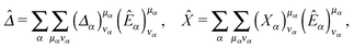 | (21) |
with which orthonormality-conserving spin-orbital variations and time derivatives can be written as| | 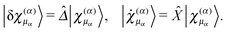 | (22) |
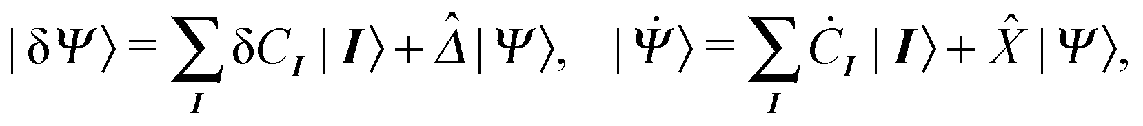
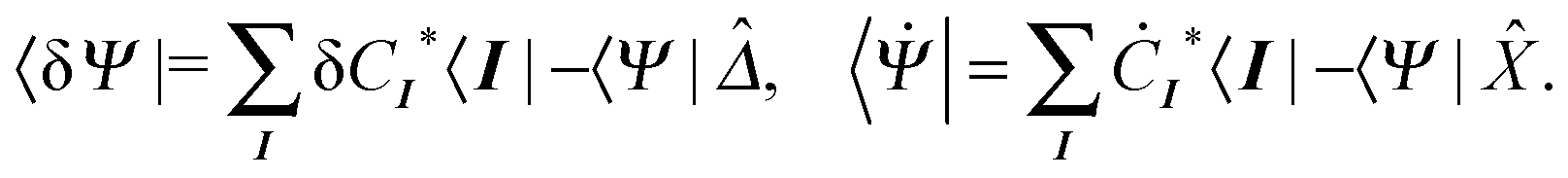
Then, the variation and time derivative of total state are compactly given by,7,10,24| | 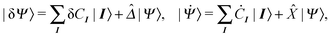 | (23) |
and their Hermitian conjugates are| | 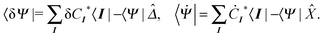 | (24) |
It follows from eqn (19) that,| | 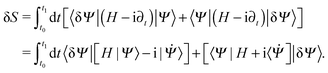 | (25) |
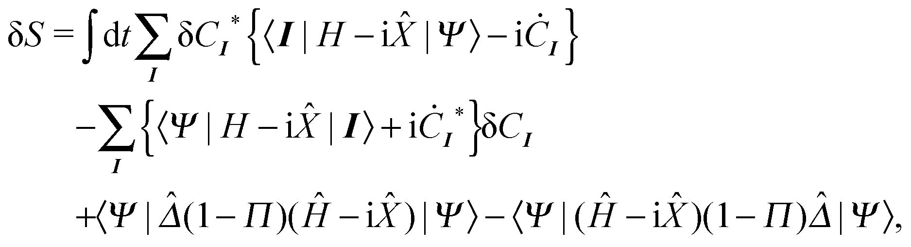
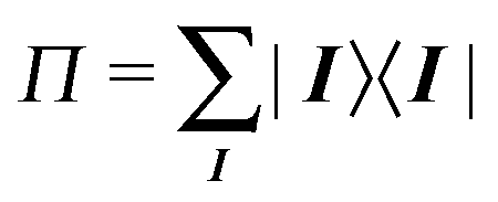
Substituting eqn (23) and (24) into this equation, after some algebraic manipulation,7,24 we obtain,| |  | (26) |
where  denotes the projector onto the CI space, i.e., the subspace of N-electron Hilbert space spanned by the configurations included in eqn (5). The action functional S should be made stationary with respect to all independent variations; {δCI, δCI*} for CI coefficients and
  for spin-orbitals.
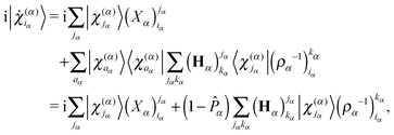
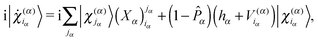
First, the EOM for CI coefficients are obtained from δS/δCI* = 0,
| | 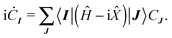 | (27) |
Requiring δ
S/δ
CI = 0 derives the complex conjugate of
eqn (27). Next from

, one obtains
| |  | (28) |
where
![[capital Pi, Greek, macron]](https://www.rsc.org/images/entities/i_char_e136.gif)
= 1 −
Π.
Eqn (28) is to be solved for
, thus determines the time derivative of spin-orbitals. We now take a closer look at
eqn (28) for the following two distinct cases:
Case 1: (μα, να) = (iα, jα)
In this case we focus on the components of the spin-orbital variations within the subspace spanned by the occupied spin-orbitals. Since  and
and  in general, one needs to directly work with eqn (28) within the occupied spin-orbital space
| |  | (29) |
In the full-CI case, where  ,
,  , eqn (29) reduces to an identity 0 = 0. Therefore, the corresponding
  may be arbitrary anti-Hermitian matrix elements, of which the simplest choice is
  .
.
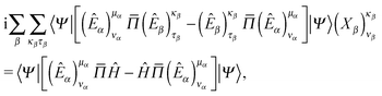
Case 2: (μα, να) = (iα, aα)
In this case we deal with the components of the spin-orbital variations outside the occupied spin-orbital space. Since 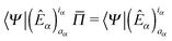 and
and  , eqn (28) becomes,
| | 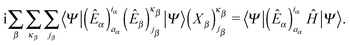 | (30) |
However, the matrix element in the left-hand side of the above equation survives only when β = α and κα = aα ∈ Ωvirα, namely  . Thus eqn (30) is simplified to
| |  | (31) |
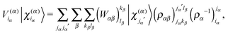
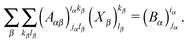
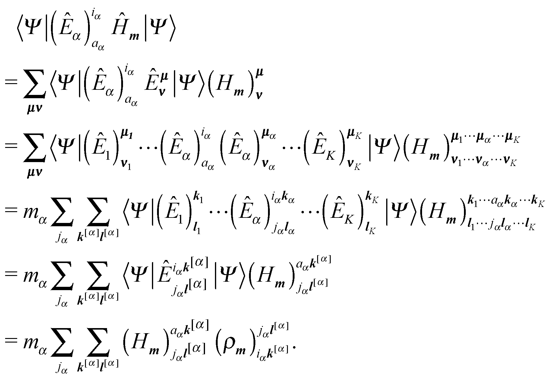
The m-body Hamiltonian contribution to the RHS of eqn (31) is evaluated as follows;| | 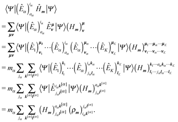 | (32) |
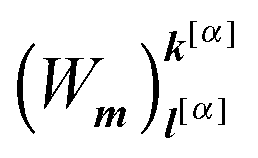
In the second line of the above equation, we note that the matrix element survives when one and only one of the mα creation operators in  refers to aα ∈ Ωvirα, and all the others to the occupied spin-orbitals. All such cases [μα,p = aα, μα,q≠p ∈ Ωoccα;1 ≤ p ≤ mα] give the same contribution since the phase (∓)p−1 [+ (−) sign for bosons (fermions), arising in (anti-)commuting the creation operators] is canceled by shifting the corresponding annihilation operator να,p, and the Hamiltonian is symmetric for interchange of particles of the same kind. The third line is thus obtained after renaming summation variables, where k[α] = (k1,…,kα,…,kK) is the array of m − 1 indices with kα = (kα,2,…,kα,mα) and kβ = (kβ,1,…,kβ,mβ) for β ≠ α, with l[α] defined similarly. The fourth line introduces the short-hand notation for the array of m indices, μαk[α] = (k1,…,μαkα,…,kK) with μαkα = (μα,kα,2,…,kα,mα) (μαl[α] is defined similarly), and the fifth line uses the definition of the m-body RDM, eqn (17).
Now the RHS of eqn (31) is given by the sum over m,
| |  | (33) |
where

is the effective one-particle operator,
| |  | (34) |
and

is given in the coordinate representation as
| |  | (35) |
where
y[α] = (
y1,…,
yα,…,
yK) is the set of
m − 1 coordinates with
yα = (
yα,2,…,
yα,mα) and
yβ = (
yβ,1,…,
yβ,mβ) for
β ≠
α, and
xαy[α] = (
y1,…,
xαyα,…,
yK) is the array of
m coordinates.
z[α] and
xα′
z[α] are defined similarly.
Finally, gathering the occupied and virtual components of the time derivative completes the derivation of the EOM for spin-orbitals
| |  | (36) |
where
is the spin-orbital projection operator onto the occupied spin-orbital space, with which the virtual space
is referenced as a whole, thus avoiding the explicit use of virtual spin-orbitals.

in the first term is to be obtained by solving
eqn (29), and, as discussed above, can be set zero in the full-CI case.
Eqn (27) for CI coefficients and
eqn (36) for spin-orbitals form fully general TD-MCSCF equations of motion, not restricted to full CI, for a system composed of any arbitrary kinds and numbers of fermions and bosons.
4 Molecules interacting with an external laser field
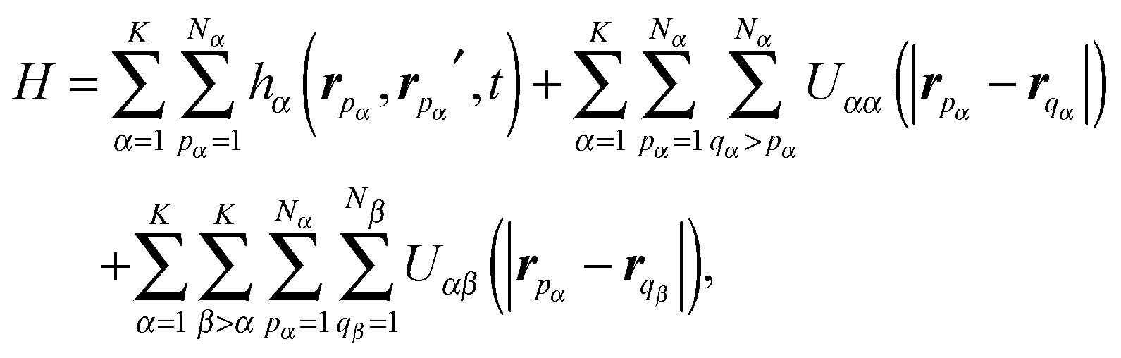
In this section we present the working equations for a molecule subject to an external laser field. Let the molecule consist of electrons and Kn different kinds of nuclei treated quantum mechanically (the kind does not necessarily corresponds to the nuclear species, see discussion below), and Ncl nuclei treated as a classical point charge. For clarity and notational simplicity, we assign the electrons to the first kind of particle (α = 1), and kinds α = 2, 3,…,K represent quantum nuclei with K = 1 + Kn. The numbers of identical particles are, as before, denoted by {Nα}. Then the number of electrons is N1, the number of quantum nuclei is  , and the total number of atoms is Natom = Nn + Ncl. We use atomic units in this section.
The spin-independent molecular Hamiltonian in the coordinate representation is given by
| | 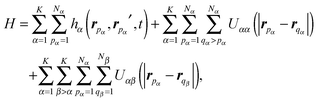 | (37) |
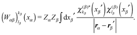
where
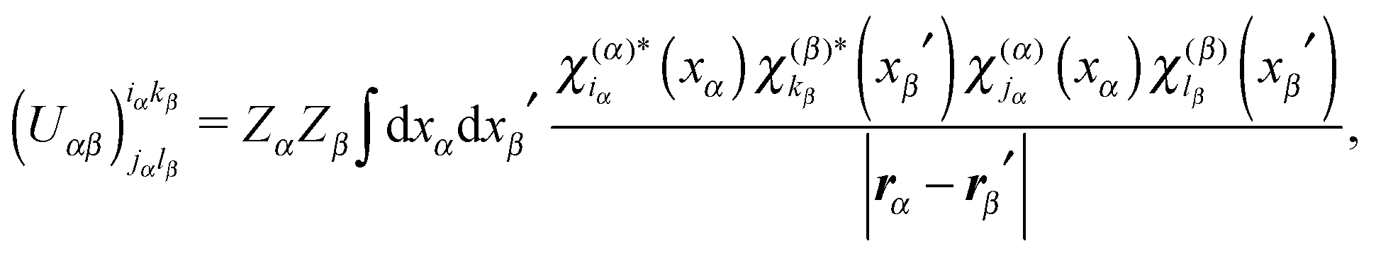
Uαβ(
r) =
ZαZβ/
r is the Coulomb interaction with
Zα being the electric charge, and
| | 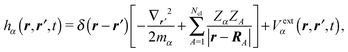 | (38) |
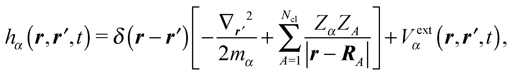
is the one-particle Hamiltonian composed of the kinetic energy [the first term with
mα being the mass (not to be confused with the number of particles)], Coulomb interaction with classical nuclei with the charges {
ZA} located at {
RA} (the second term), and the time-dependent laser-particle interaction
Vextα, given,
e.g., within the dipole approximation either in the length gauge (LG) or in the velocity gauge (VG), by
| | | Vextα,LG(r,r′,t) = −δ(r − r′)ZαE(t)r, | (39) |
| | 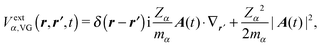 | (40) |
where
E(
t) is the laser electric field, and
is the vector potential.
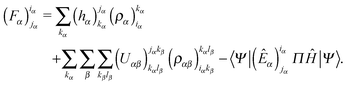
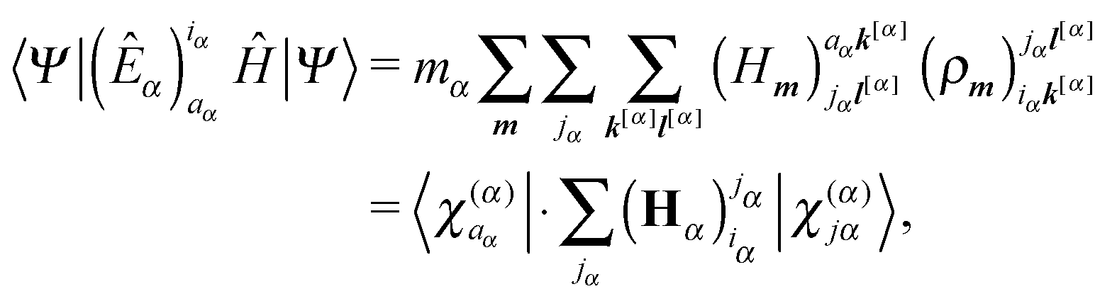
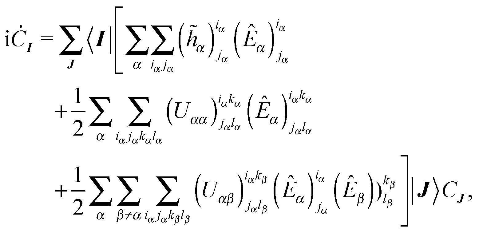
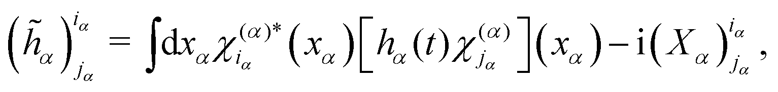
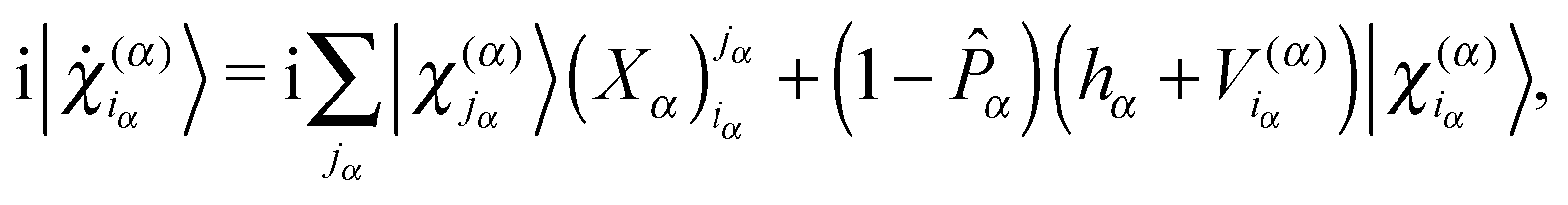
The general formulation of Section 3 is readily applicable to the molecular Hamiltonian of eqn (37). The CI EOM reads
| | 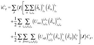 | (41) |
where
| | 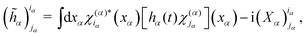 | (42) |
| | 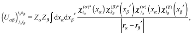 | (43) |
with
xα = (
rα,
σα) being the composite spatial- and spin-coordinates, and the EOM for spin-orbitals is given by
| |  | (44) |
where the one-body contribution to the second term of
eqn (36) is extracted to lead to

by noting

, and
| |  | (45) |
| |  | (46) |
Finally, eqn (29) is formulated as the linear system of equations,
| |  | (47) |
where
,
, with
| |  | (48) |
| |  | (49) |
In order for
eqn (47) to be solvable (with non-singular coefficient matrix
A), one needs a systematic method of constructing non-full-CI space analogous to the TD-ORMAS method
10 for electrons. We shall discuss this issue in the future publication.
Equations of motions (41) and (44), with the matrix eqn (47), define the general TD-MCSCF method, not restricted to full CI, for molecules interacting with an external field. Our formulation is very flexible; it includes as special cases both the electron dynamics at the classical-nuclei approximation (Nn = 0, Ncl = Natom) and the full quantum molecular dynamics (Nn = Natom, Ncl = 0). Furthermore, it allows various approaches to the same physical problem; e.g., the same nuclear species in the molecule can be treated either as identical particles or distinguishable ones to investigate the physical outcomes of the particle statistics during the course of laser-molecule interactions.
5 Numerical examples
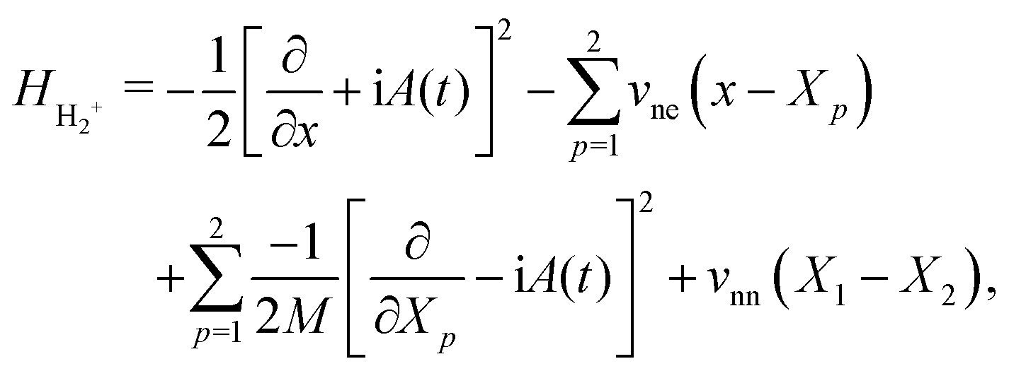
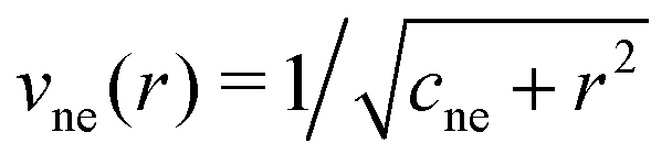
In order to demonstrate the utility of the TD-MCSCF method for an exactly solvable system, in this section, we consider a one-dimensional model hydrogen molecular ion with the singlet protonic spin configuration (1D para-H2+), driven by an intense near-infrared laser pulse. The Hamiltonian within the dipole approximation in the velocity gauge is given in terms of electron coordinate x and proton coordinates X1, X2 by| | 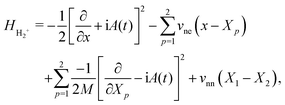 | (50) |
where M denotes the proton mass, and 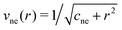 , and
, and  are the electron–proton and proton–proton soft Coulomb potentials, respectively. Following ref. 25, we set cne = 1 and cnn = 0.03, and transform the coordinates as z = x − (X1 + X2)/2, X = (X1 + X2)/2, and R = X1 − X2. Neglecting the terms involving X, ∂/∂X and transforming into the length gauge lead to the reduced Hamiltonian,25
| | 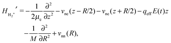 | (51) |
with μe = 2M/(2M + 1) and qeff = −(2M + 2)/(2M + 1). This Hamiltonian was used, e.g., for investigating charge-resonance enhanced ionization,25 but application of the multiconfiguration method to this system in the context of highly nonlinear laser-driven dynamics such as high-harmonic generation has not previously been reported to the best of our knowledge.
Let us compare the following treatments: (1) numerically exact solution of the time-dependent Schrödinger equation (TDSE) for the spatial part Ψexact(z,R,t) of the 1D × 1D wavefunction by discretizing electron coordinate z and nuclear distance R with constant grid spacing δz = 0.4 and δR = 0.2, respectively, within the simulation volume |z| < 640 and |R| < 80, (2) the electron only dynamics by solving for electronic wavefunction Ψfixed(z,t) given the first line of eqn (51) with a fixed (near to equilibrium) internuclear distance R0 = 2.6 [fixed (classical point) nuclei approximation], and (3) TD-MCSCF method with the total wavefunction given by
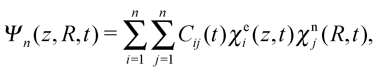
| | 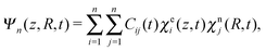 | (52) |
using
n occupied spatial orbitals both for the electron and the
R degree-of-freedom of the protons. Note that
n = 1 corresponds, in this example, to the time-dependent Hartree approximation,
ΨTDH =
Ψ1 =
χe1(
z,
t)
χn1(
R,
t). (4) Based on this TDH method we also consider the frozen (quantum) nuclei approximation, where the protonic orbital is fixed to the initial form,
| | | Ψfrozen(z,R,t) = χe1(z,t)χn1(R,0). | (53) |
The same spatial discretization as that in the first treatment is applied to the latter three. For each method described above we first obtain the ground state by imaginary time propagation of the respective EOM, and then investigate the molecular dynamics induced by the NIR laser pulse with a peak intensity of 10
14 W cm
−2 and a central wavelength of 800 nm, with a sin
2 envelop of the foot-to-foot pulse duration of 12 optical cycles. The TDH ground state orbitals are used as initial orbitals in
eqn (53).
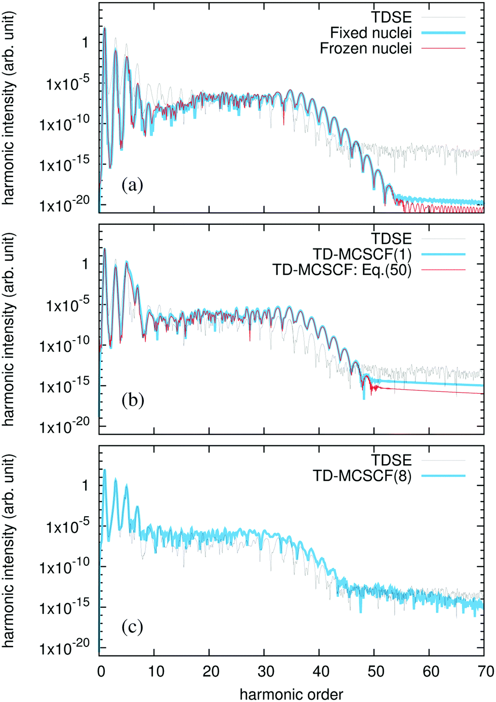
Fig. 1 shows the time evolution of the dipole acceleration a(t) = d2〈Ψ(t)|z|Ψ(t)〉/dt2 computed using the Ehrenfest theorem. As shown in Fig. 1(a), both fixed-nuclei (light blue curve) and frozen-nuclei (red) approximations strongly underestimate the nonlinear response seen in the TDSE result (black), which suggests the importance of the dynamical quantum treatment of nuclei. The TD-MCSCF method with n = 1, or TDH [Fig. 1(b)] provides improved description of the nonlinear response, but still fails to quantitatively reproduce the TDSE result. The TD-MCSCF method with n = 8 [Fig. 1(c)], on the other hand, produces the dipole acceleration that agrees with the TDSE result nearly perfectly, on the scale of the figure. The HHG spectra calculated as the modulus squared of the Fourier transform of the dipole acceleration are shown in Fig. 2. The fixed and frozen nuclei approximations underestimate the intensity of the first few harmonics, while overestimating the higher plateau (the cutoff position is estimated to be the 39th harmonic from the Lewenstein model26) [Fig. 2(a)], both suggesting an important contribution from (more polarizable and loosely bound) the larger |R| region in the TDSE result. The TD-MCSCF spectrum with increasing n [shown for n = 1 (Fig. 2(b)) and n = 8 (Fig. 2(c))] shows increasingly better agreement with the TDSE one, and the TD-MCSCF method with n = 8 nicely reproduces the overall spectrum obtained using the TDSE simulations, especially for low-order harmonics, albeit with a still remaining slight overestimation of the plateau intensity which implies a strong electron–proton correlation.
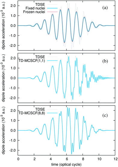 |
| | Fig. 1 Time evolution of the dipole acceleration of one-dimensional H2+ exposed to a laser pulse with a wavelength of 800 nm and an intensity of 1.0 × 10¹⁴ W cm−2. Comparison of the results of fixed nuclei and frozen nuclei approximations (a), TD-MCSCF method with n = 1 (b), and TD-MCSCF method with n = 8 (c) with numerically exact TDSE results. | |
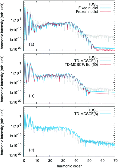 |
| | Fig. 2 The HHG spectra of one-dimensional H2+ for the same laser pulse and simulation methods as those in Fig. 1. Comparison of the results of fixed nuclei and frozen nuclei approximations (a), TD-MCSCF method with n = 1 (b), and TD-MCSCF method with n = 8 (c) with numerically exact TDSE results. Also shown in (b) is the result of the TD-MCSCF method directly applied for the Hamiltonian of eqn (50) with one electronic orbital and two protonic orbitals. | |
Finally, also plotted in Fig. 2(b) with a red line is the result of TD-MCSCF method directly applied to the Hamiltonian of the original coordinate, eqn (50), with one electronic orbital and two protonic orbitals to expand the three-particle wavefunction Ψ(x,X1,X2), using the method described in ref. 19 to eliminate the translational degree of freedom. We find a remarkable agreement between the results from the original Hamiltonian eqn (50) and the reduced Hamiltonian eqn (51). The former approach can be applied to more complex systems in general.
6 Summary
We have developed a fully general ab initio TD-MCSCF approach to describe the dynamics of a many-body system that is a mixture of any arbitrary kinds and numbers of fermions and bosons subject to an external field. In this approach, the total wave function is expanded in terms of configurations constructed from time-dependent single-particle spin-orbitals. The expansion is not limited to the full-CI one, and the configurations used in the expansion can be specified in terms of the whole mixture. The equations of motion for the CI coefficients and spin-orbitals have been derived, based on the time-dependent variational principle. Furthermore, we have presented the working equations applicable to the investigation of the ultrafast dynamics in a molecule irradiated by intense laser fields and/or ultrashort XUV pulses.
The present framework is highly flexible. For example, we can treat identical nuclei in spatially separated subdomains of a molecule as different particle kinds. We can also treat heavy nuclei and incident projectiles as classical particles18 instead of quantum ones. The latter may be handled as an external field as well. This flexibility will be useful for unraveling the physical mechanisms underlying the phenomena under investigation.27 As a future prospect, an introduction of a CI space that adaptively changes following the dynamics as well as an inclusion of particle conversion16 would enable even more efficient and flexible simulations.
Whereas our original motivation lies in ab initio simulations of the electron–nuclear dynamics in molecules driven by a laser pulse, our method will be applicable to a wide variety of problems far beyond. Especially, the Hamiltonian can contain non-local terms and involve many-body (more than two-body) interactions. Thus, it may also find applications in cold-atom/cold-molecule physics and nuclear physics.
Conflicts of interest
There are no conflicts of interest to declare.
Acknowledgements
We thank Joachim Burgdörfer for helpful discussions. This research was supported in part by a Grant-in-Aid for Scientific Research (Grants No. 25286064, 26390076, 26600111, 16H03881, and 17K05070) from Japan Society for the Promotion of Science and also by the Photon Frontier Network Program of the Ministry of Education, Culture, Sports, Science and Technology of Japan. This research was also partially supported by the Center of Innovation Program from the Japan Science and Technology Agency, JST, and by CREST (Grant No. JPMJCR15N1), JST. R. A. gratefully acknowledges support from the Graduate School of Engineering, The University of Tokyo, Doctoral Student Special Incentives Program (SEUT Fellowship).
References
- P. Agostini and L. F. DiMauro, Rep. Prog. Phys., 2004, 67, 1563 CrossRef.
- F. Krausz and M. Ivanov, Rev. Mod. Phys., 2009, 81, 163–234 CrossRef.
- L. Gallmann, C. Cirelli and U. Keller, Annu. Rev. Phys. Chem., 2013, 63, 447 CrossRef PubMed.
- T. Kato and H. Kono, Chem. Phys. Lett., 2004, 392, 533–540 CrossRef CAS.
- J. Caillat, J. Zanghellini, M. Kitzler, O. Koch, W. Kreuzer and A. Scrinzi, Phys. Rev. A: At., Mol., Opt. Phys., 2005, 71, 012712 CrossRef.
- K. L. Ishikawa and T. Sato, IEEE J. Sel. Top. Quantum Electron., 2015, 21, 1–16 CrossRef.
- T. Sato and K. L. Ishikawa, Phys. Rev. A: At., Mol., Opt. Phys., 2013, 88, 023402 CrossRef.
- T. Sato, K. L. Ishikawa, I. Březinová, F. Lackner, S. Nagele and J. Burgdörfer, Phys. Rev. A, 2016, 94, 023405 CrossRef.
- H. Miyagi and L. B. Madsen, Phys. Rev. A: At., Mol., Opt. Phys., 2014, 89, 063416 CrossRef.
- T. Sato and K. L. Ishikawa, Phys. Rev. A: At., Mol., Opt. Phys., 2015, 91, 023417 CrossRef.
- H.-D. Meyer, U. Manthe and L. Cederbaum, Chem. Phys. Lett., 1990, 165, 73–78 CrossRef CAS.
- I. S. Ulusoy and M. Nest, J. Chem. Phys., 2012, 136, 054112 CrossRef PubMed.
- M. Nest, Chem. Phys. Lett., 2009, 472, 171–174 CrossRef CAS.
- O. E. Alon, A. I. Streltsov and L. S. Cederbaum, Phys. Rev. A, 2007, 76, 062501 CrossRef.
- O. E. Alon, A. I. Streltsov and L. S. Cederbaum, J. Chem. Phys., 2007, 127, 154103 CrossRef PubMed.
- O. E. Alon, A. I. Streltsov and L. S. Cederbaum, Phys. Rev. A: At., Mol., Opt. Phys., 2009, 79, 022503 CrossRef.
- O. E. Alon, A. I. Streltsov, K. Sakmann, A. U. Lode, J. Grond and L. S. Cederbaum, Chem. Phys., 2012, 401, 2–14 CrossRef CAS.
- T. Kato and K. Yamanouchi, J. Chem. Phys., 2009, 131, 164118 CrossRef PubMed.
- H. Nakai, M. Hoshino, K. Miyamoto and S. Hyodo, J. Chem. Phys., 2005, 122, 164101 CrossRef PubMed.
- H. Nakai, M. Hoshino, K. Miyamoto and S. aki Hyodo, J. Chem. Phys., 2005, 123, 237102 CrossRef.
- A. Dalgarno and G. Victor, Proc. R. Soc. London, Ser. A, 1966, 291–295 CrossRef CAS.
- P.-O. Löwdin and P. Mukherjee, Chem. Phys. Lett., 1972, 14, 1–7 CrossRef.
- R. Moccia, Int. J. Quantum Chem., 1973, 7, 779–783 CrossRef.
- R. P. Miranda, A. J. Fisher, L. Stella and A. P. Horsfield, J. Chem. Phys., 2011, 134, 244101 CrossRef CAS PubMed.
- E. Khosravi, A. Abedi and N. T. Maitra, Phys. Rev. Lett., 2015, 115, 263002 CrossRef PubMed.
- M. Lewenstein, P. Balcou, M. Y. Ivanov, A. L'Huillier and P. B. Corkum, Phys. Rev. A: At., Mol., Opt. Phys., 1994, 49, 2117 CrossRef.
- I. Tikhomirov, T. Sato and K. L. Ishikawa, Phys. Rev. Lett., 2017, 118, 203202 CrossRef PubMed.
|
| This journal is © the Owner Societies 2017 |
Click here to see how this site uses Cookies. View our privacy policy here. 
 Open Access Article
 This Open Access Article is licensed under a
  ab
ab
 particles as a whole. For notational brevity, we call such a system an N-particle system, where the array of integers N = (N1N2⋯NK) carries the information of both particle kinds and the number of particles in each kind.
 , which spans the one-particle Hilbert space Ωα, is time-dependent in general. Then the N-particle Hilbert space is spanned by
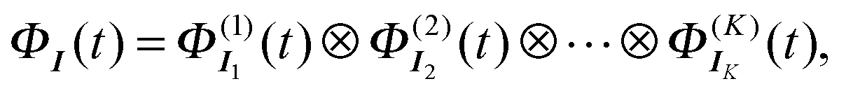
 is a determinant (or permanent) of α-kind fermions (or bosons), consisting of Nα spin-orbitals chosen from
  . We call ΦI(t) the I’s configuration, where I = I1I2⋯IK is considered, at the moment, to collectively label the chosen spin-orbitals. The objective of this paper is to formulate the TD-MCSCF theory of the N-particle system within the ansatz of total wavefunction analogous to that for the electronic system, eqn (1), but using the configurations of eqn (2).
 associated with
  . These operators obey the (anti-)commutation relations of bosons (fermions),
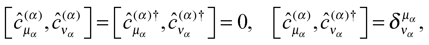
 is split into nα (≥Nα for fermions) occupied spin-orbitals
  and remaining virtual spin-orbitals
  . We call the subspace of Ωα spanned by occupied spin-orbitals the occupied spin-orbital space Ωoccα, and that spanned by virtual spin-orbitals the virtual spin-orbital space Ωvirα, where Ωα = Ωoccα ⊕ Ωvirα. The total state Ψ(t) is expressed as a superposition of configurations ΦI(t) of eqn (2), but constructed from occupied spin-orbitals only. Thus we write
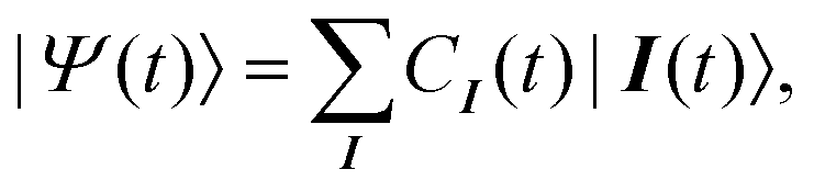
 . Note that Iα,iα ∈ {0,1} for fermions. Here and in what follows, we use indices iα, jα, kα,… for occupied (Ωoccα), aα, bα, cα,… for virtual (Ωvirα), and μα, να, κα, τα,… for general (Ωα) spin-orbitals of kind α. The indices pα, qα will be used for numbering the coordinates.

 ),
),
 , with
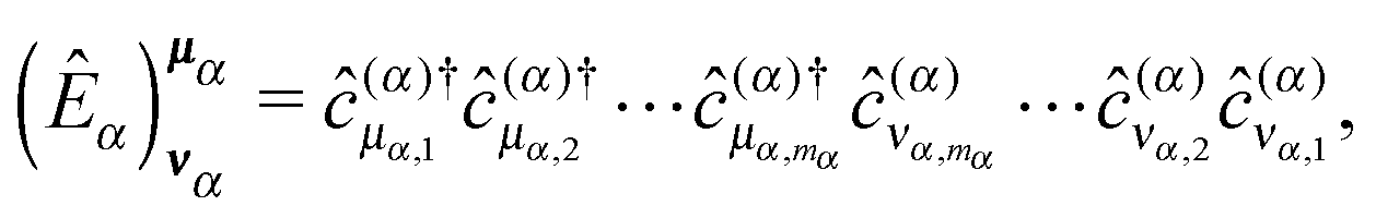


 denotes the projector onto the CI space, i.e., the subspace of N-electron Hilbert space spanned by the configurations included in eqn (5). The action functional S should be made stationary with respect to all independent variations; {δCI, δCI*} for CI coefficients and
  for spin-orbitals.
 , one obtains
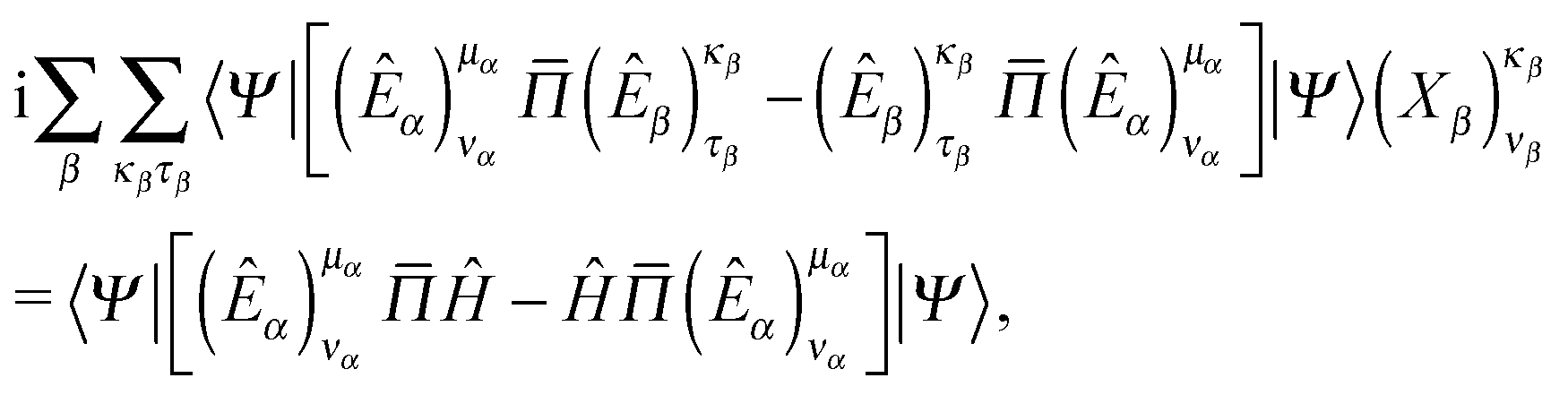
 , thus determines the time derivative of spin-orbitals. We now take a closer look at eqn (28) for the following two distinct cases:
 and
and  in general, one needs to directly work with eqn (28) within the occupied spin-orbital space
 ,
,  , eqn (29) reduces to an identity 0 = 0. Therefore, the corresponding
  may be arbitrary anti-Hermitian matrix elements, of which the simplest choice is
 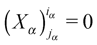 .
.
 and
and 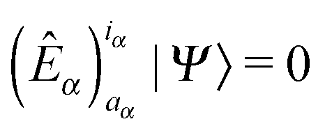 , eqn (28) becomes,
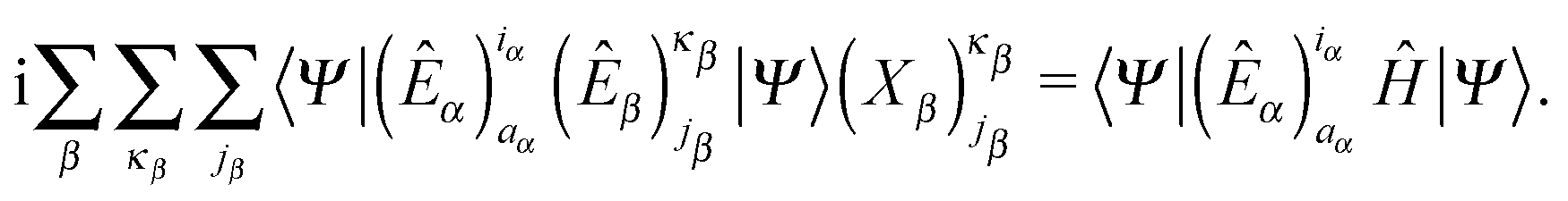
 . Thus eqn (30) is simplified to
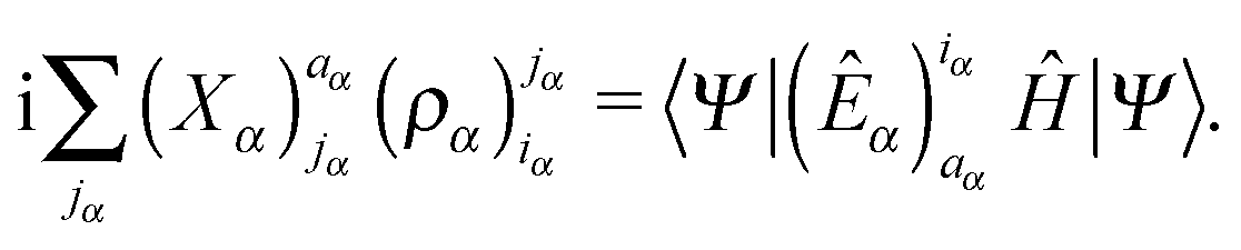
 refers to aα ∈ Ωvirα, and all the others to the occupied spin-orbitals. All such cases [μα,p = aα, μα,q≠p ∈ Ωoccα;1 ≤ p ≤ mα] give the same contribution since the phase (∓)p−1 [+ (−) sign for bosons (fermions), arising in (anti-)commuting the creation operators] is canceled by shifting the corresponding annihilation operator να,p, and the Hamiltonian is symmetric for interchange of particles of the same kind. The third line is thus obtained after renaming summation variables, where k[α] = (k1,…,kα,…,kK) is the array of m − 1 indices with kα = (kα,2,…,kα,mα) and kβ = (kβ,1,…,kβ,mβ) for β ≠ α, with l[α] defined similarly. The fourth line introduces the short-hand notation for the array of m indices, μαk[α] = (k1,…,μαkα,…,kK) with μαkα = (μα,kα,2,…,kα,mα) (μαl[α] is defined similarly), and the fifth line uses the definition of the m-body RDM, eqn (17).
 is the effective one-particle operator,
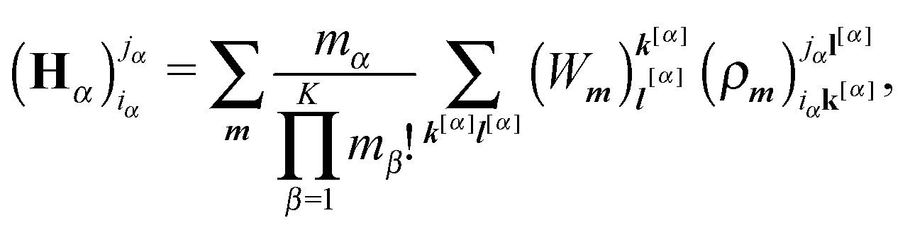
 is given in the coordinate representation as
 is the spin-orbital projection operator onto the occupied spin-orbital space, with which the virtual space
 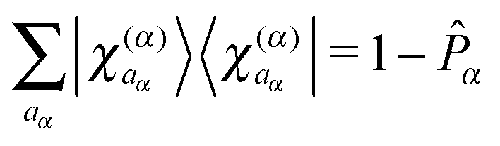 is referenced as a whole, thus avoiding the explicit use of virtual spin-orbitals.
  in the first term is to be obtained by solving eqn (29), and, as discussed above, can be set zero in the full-CI case. Eqn (27) for CI coefficients and eqn (36) for spin-orbitals form fully general TD-MCSCF equations of motion, not restricted to full CI, for a system composed of any arbitrary kinds and numbers of fermions and bosons.
 , and the total number of atoms is Natom = Nn + Ncl. We use atomic units in this section.

 is the vector potential.
 by noting
  , and
, and


 ,
,  , with

 , and
, and  are the electron–proton and proton–proton soft Coulomb potentials, respectively. Following ref. 25, we set cne = 1 and cnn = 0.03, and transform the coordinates as z = x − (X1 + X2)/2, X = (X1 + X2)/2, and R = X1 − X2. Neglecting the terms involving X, ∂/∂X and transforming into the length gauge lead to the reduced Hamiltonian,25