
 Open Access Article
 This Open Access Article is licensed under a
 Creative Commons Attribution 3.0 Unported Licence
Back-exchange: a novel approach to quantifying oxygen diffusion and surface exchange in ambient atmospheres
Samuel J.
Cooper
 *a,
Mathew
Niania
b,
Franca
Hoffmann
c and
John A.
Kilner
b
*a,
Mathew
Niania
b,
Franca
Hoffmann
c and
John A.
Kilner
b
aDyson School of Design Engineering, Imperial College London, London, SW7 1NA, UK. E-mail: samuel.cooper@imperial.ac.uk
bDepartment of Materials, Imperial College London, London, SW7 2BP, UK
cDPMMS, Centre for Mathematical Sciences, University of Cambridge, Wilberforce Road, Cambridge, CB3 0WA, UK
First published on 27th April 2017
Abstract
A novel two-step Isotopic Exchange (IE) technique has been developed to investigate the influence of oxygen containing components of ambient air (such as H2O and CO2) on the effective surface exchange coefficient (k*) of a common mixed ionic electronic conductor material. The two step ‘back-exchange’ technique was used to introduce a tracer diffusion profile, which was subsequently measured using Time-of-Flight Secondary Ion Mass Spectrometry (ToF-SIMS). The isotopic fraction of oxygen in a dense sample as a function of distance from the surface, before and after the second exchange step, could then be used to determine the surface exchange coefficient in each atmosphere. A new analytical solution was found to the diffusion equation in a semi-infinite domain with a variable surface exchange boundary, for the special case where D* and k* are constant for all exchange steps. This solution validated the results of a numerical, Crank-Nicolson type finite-difference simulation, which was used to extract the parameters from the experimental data. When modelling electrodes, D* and k* are important input parameters, which significantly impact performance. In this study La0.6Sr0.4Co0.2Fe0.8O3−δ (LSCF6428) was investigated and it was found that the rate of exchange was increased by around 250% in ambient air compared to high purity oxygen at the same pO2. The three experiments performed in this study were used to validate the back-exchange approach and show its utility.
1 Introduction
The self-diffusion coefficient, D*, and the effective surface exchange coefficient, k*, of oxygen conducting materials are important parameters when selecting materials for applications such as Solid Oxide Fuel Cells (SOFC) electrodes, oxygen separation membranes and sensors. The measurement of D* and k* by Isotopic Exchange Depth Profiling (IEDP) was first described by Kilner et al. in 1984.1 The technique has since been greatly refined to allow for the investigation of higher diffusivity materials using linescans2 and parallel detection of secondary ions using ToF-SIMS.3 The IEDP method described in ref. 1 has a key limitation, which the approach presented in this work aims to resolve. The use of high purity isotopically enriched oxygen gas is significantly restricted by its cost and as such it is common to reclaim the gas used after each experiment. This precludes the use of enriched multicomponent gas mixtures, which are needed to model typical operating environments for many common applications. Furthermore, there is some discrepancy in the literature over values of D* and k* for widely studied materials, such as the mixed conductor La0.6Sr0.4Co0.2Fe0.8O3−δ (LSCF6428). This may be the result of trace gasses present during the exchange, which are not always reported.To extract D* and k* from experimental isotopic fraction data, the appropriate solution to the diffusion equation, eqn (1), is fitted by a non-linear least squares method. This expression was originally derived by Carslaw and Jaeger4 as the solution to sys. 3, but was more famously communicated by Crank in his book “The Mathematics of Diffusion” (hence “Crank's solution”).5
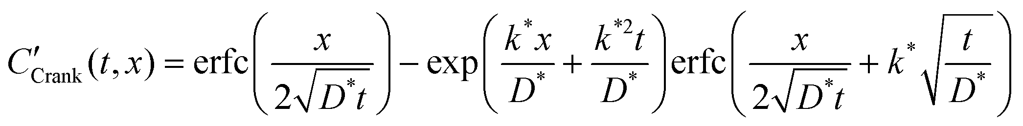 | (1) |
This function is the solution to the 1-dimensional (1D) diffusion equation in a semi-infinite domain, with a surface exchange boundary and uniform initial conditions, where C′ is the normalised isotopic fraction found using eqn (2) (N.B. this normalisation notation is consistent throughout this paper and the dash should not be confused with a derivative); t > 0 is the duration of the exchange; and x ≥ 0 is the depth of the profile into the sample from the exchange surface.
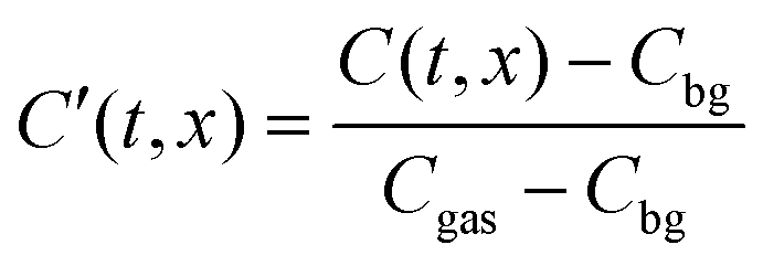 | (2) |
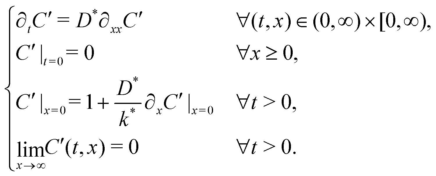 | (3) |
The background isotopic fraction and that of the enriched exchange gas, Cbg and Cgas respectively, are required for the normalisation in eqn (2). System 3 uses the notation ∂t to represent a partial derivative with respect to t.
2 Back-exchange
The back-exchange technique presented in this study starts with a conventional exchange in an 18O enriched gas, following the protocol described in ref. 3, but then includes a second step where the sample is exposed to any unenriched gas environment. In order to draw a meaningful comparison, the temperature and partial pressure of oxygen should be the same for all exchange steps. To the authors' knowledge, there is no analytical solution available in the literature for this kind of two-step exchange process; however, a solution has been derived here for the special case where the values of D* and k* are the same for both exchanges.2.1 Analytical solution
Many diffusion problems are amenable to solution by superposition, but due to the exchange type (Robin) boundary condition, this approach was non-trivial. The system describing the second exchange step is contained in sys. 4, where CCrank′(ϕ1,x) is the result of eqn (1), keeping the values of D* and k* the same for the first and second exchange steps, after ϕ1 seconds. Although variable t is used for exchange time in eqn (1), the non-ideal nature of real exchange experiments (i.e. finite heating and cooling rates) requires an “effective exchange time” to be calculated from temperature time series data. The variable ϕi is used to describe this adjusted time, in exchange step i, and is based on the linearisation described by Killoran.6 In the following discussion, time t is assumed to start at the beginning of the final exchange step, with the results of previous exchanges effecting only the initial conditions.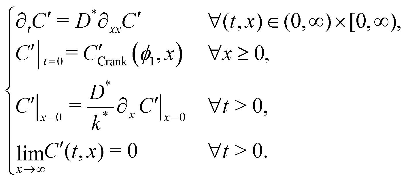 | (4) |
System 4, has two key differences from the single step system. Firstly, by considering the system time to start at the beginning of the second exchange, the initial condition is the Crank solution resulting from the first exchange, rather than a uniform distribution at background level. Secondly, the boundary condition no longer has the Cgas stimulation and now simply sets the surface gradient proportional to the current surface concentration (Neumann boundary condition).
The existence and uniqueness of a weak solution, in the sense of distributions, to this system follows from the Lax–Milgram Theorem once it has been converted into Laplace space.7 The solution was found by considering the following two physical constraints. Firstly, that the diffusion length, which is the convenient measure of the degree of penetration of a profile, must be approximately  ; secondly, that C′ must be positive for all values of t and ϕ1. The solution found is given by,
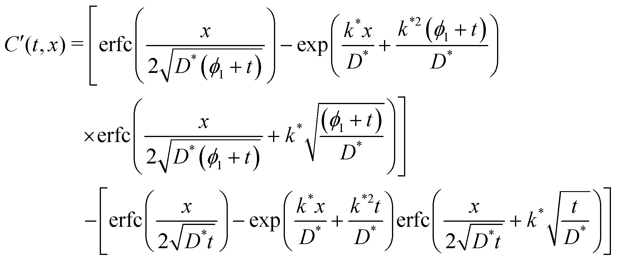 | (5) |
| C′(t,x) = CCrank′((ϕ1 + t),x) − CCrank(t,x) | (6) |
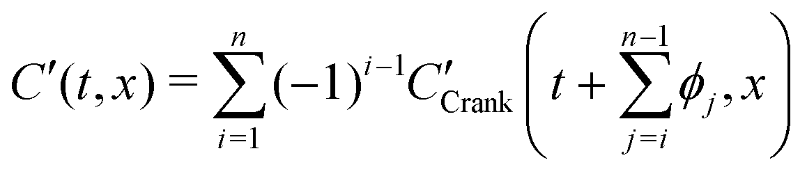
By simple differentiation and substitution, it can be shown that eqn (5) is the unique solution to sys. 4. Furthermore, this approach can be extended to n exchanges, eqn (7), where D* and k* are constant; ϕj is the duration of exchange j; and the normalised gas concentration at the boundary alternates between 1 and 0 at each step.
 | (7) |
Although useful for validation purposes, these analytical solutions are only suitable for fitting profiles where D* and k* are the same in each exchange step. The following section describes a numerical scheme constructed for fitting all other cases.
2.2 Numerical methods
In order to generate profiles to use for fitting the experimental back-exchange data with multiple D* and k* values, a 1D Crank-Nicolson (CN)8 type finite-difference simulation was used to numerically solve the system. The CN approach was chosen for its numerical stability and O(Δx2,Δt2) accuracy. For these line-scan type datasets, the spatial step, Δx, was fixed to correspond to the experimental data raster spacing, while the time step, Δt, was adjusted to preserve accuracy. The ghost node concept, described in more detail in ref. 9, was employed at both ends of the simulation domain. A ghost node is a fictitious extra node located outside the boundary of the system, which is not evaluated directly or stored in memory, but instead used to preserve the boundary condition by extrapolation, which maintains the O(Δx2,Δt2) accuracy throughout the domain.To ensure that the semi-infinite boundary was modelled accurately, a hybridised boundary condition was utilised, which involved running the simulation twice (once with a mirror boundary (Neumann, ∂xC′ = 0) and once with a fixed boundary (Dirichlet, C′ = 0)) and taking the mean (validated using the analytical form described above). However, as all the profiles measured in this study are very close to C′ = 0 at the edge of the analysis area, the choice of this boundary condition was of minimal significance.
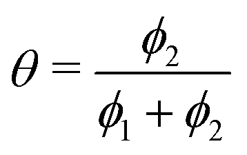
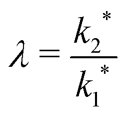
The simulation was used to explore the space of possible profiles, Fig. 1, under the constraint that D* was constant between the two exchanges, which is a property we expect from the systems investigated here, i.e. constant temperature and pO2. Seven families of curves were generated at equally spaced values of the exchange time ratio, θ, defined as,
 | (8) |
 | (9) |
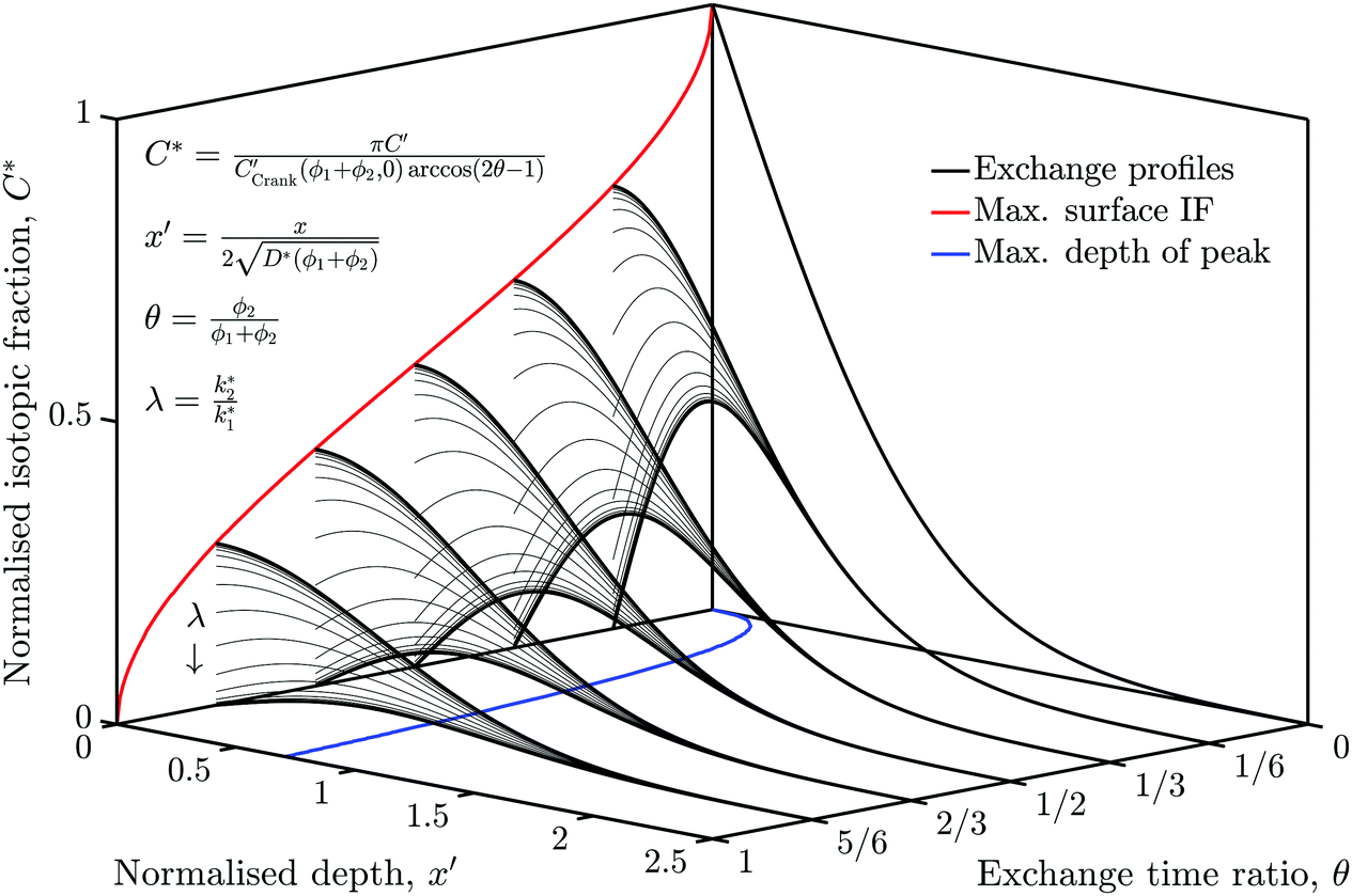 | ||
| Fig. 1 The space of possible back-exchange profiles under the constraint that D* was constant between the two exchanges. At each exchange time ratio, θ, a family of profiles was generated by varying the value of λ, which is the ratio of k2* to k1*. This graph also shows the sigmoid nature of the maximum surface value of the isotopic fraction as well as the maximum depth of the profiles' peak at each value of θ. | ||
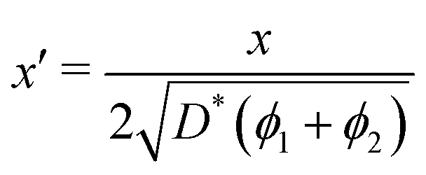
In order to allow Fig. 1 to generalise to all possible back-exchange scenarios (with D2* = D1*), the isotopic fraction required an additional normalisation step defined by,
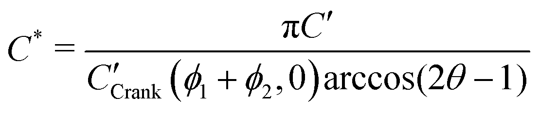 | (10) |
 | (11) |
All the required normalisation equations, described above, have been inset into Fig. 1 for convenience.
2.3 Fitting
A Nelder–Mead simplex algorithm,10 which is a non-linear, least squares approach, implemented in the MatLab fminsearch function,11 was used to fit the CN generated profiles to the experimental isotopic fraction data. The curves were fitted within a region of interest (ROI) between the surface and x′ = 2 for all profiles, to ensure that the reported values of the coefficient of determination, R2, were comparable (N.B. using data beyond x′ = 2 for fitting will force R2 to be misleadingly high for this type of problem). This required a certain degree of iteration of the fitting process as the new values of D* altered the derived location of x′ = 2.In order to efficiently fit the back-exchange data with the CN derived profiles, it is beneficial to select initial values of D* and k* with the correct order of magnitude. This is achieved by first fitting the data with the relevant analytical solution described earlier in this section and then using the results of this much faster method to initialise a second fitting using the CN profiles.
3 Experimental
The exchange experiments were conducted using the protocol described by DeSouza et al. for oxygen isotopic exchange in dense ceramic pellets.3 LCSF powder was pressed and sintered at 1250 °C for 8 h (using a heating rate of 300 °C h−1) into cuboid pellets with dimensions 2 mm × 2 mm × 5 mm (H × W × D). This geometry allowed us to assume a 1D system when modelling, as the expected depth of x′ = 2 (where C < 0.005 for all k*) was <500 μm. The pellets were then ground and polished to a mirror finish on one face using sequentially finer grades of polishing media. The grinding process was carried out using P800 grade (c. 22 μm particle size), P1200 (c. 15 μm particle size) and P2400 (c. 10 μm particle size) silicon carbide paper with water as a lubricant. After the grinding process, the samples were then polished sequentially using water based diamond suspensions with particle sizes of 6 μm, 3 μm, 1 μm and 0.25 μm. Care was taken not to skip grades to ensure not only that the surface was smooth, but also that the mechanical damage induced by each step was removed by the following step.Before the first exchange, each pellet was annealed in research grade 99.999% pure dry oxygen (16O) at the desired experimental temperature and oxygen partial pressure. By doing so, the oxygen vacancy concentration of the sample is fixed and ensures chemical equilibrium with the following exchanges. The pre-anneal time is calculated to be ten times that of the first exchange to provide a sufficiently large region with a constant oxygen non-stoichiometry. In order to determine accurately the effect of the atmosphere in the second exchange step, strict precautions were taken to ensure that the pre-anneal step and first exchange were undertaken in a dry, very high purity oxygen atmospheres. All experiments were performed in a bakeable ultra high vacuum exchange apparatus fabricated from stainless components and sealed with “conflat” flanges. Before each experimental step, the exchange volume was evacuated to a pressure of <4 × 10⁻⁷ mbar using a vacuum system employing a turbomolecular pump backed by a dry membrane pump to reduce the chance of back-streamed oil vapour. The 18O enriched oxygen for the exchanges was derived from a 5 Å molecular sieve reservoir, which ensured that the gas was dry (c. 1 vppm water). The samples were not re-polished between exchanges.
Three experiments, illustrated in Fig. 2, were performed using an initial static volume partial pressure of 200 mbar and a nominal annealing temperature of 785 °C. Experiments A and B were used to validate the back-exchange approach; experiment C was used to demonstrate its utility by investigating the effect of ambient air on the exchange process:
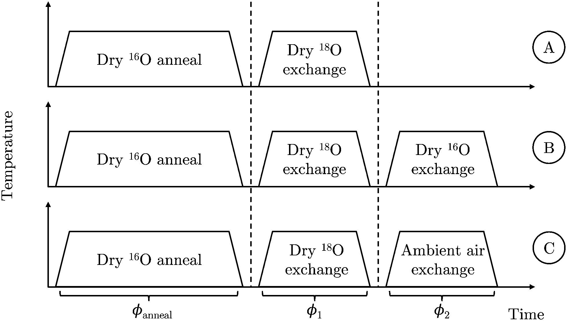 | ||
| Fig. 2 Schematic representation of the three back-exchange validation experiments. | ||
A. Dry 18O exchange ⇒ ToF-SIMS
B. Dry 18O exchange ⇒ Dry 16O exchange ⇒ ToF-SIMS
C. Dry 18O exchange ⇒ Ambient air exchange ⇒ ToF-SIMS
Due to the high oxygen diffusivity of LSCF6428 it was necessary to prepare the sample for line-scan SIMS profiling2 after the final exchange. To do so, the same grinding and polishing regime was applied to a face perpendicular to the exchange surface, prior to imaging. The sample was polished to a depth greater than a predicted value of x′ = 4 to ensure analysis occurs beyond the region where the diffusion front from this face will affect the isotopic ratio.
The exposed cross-section was then imaged using a ToF-SIMS IV machine (ION-TOF GmbH, Münster, Germany), as illustrated in Fig. 3. The technique collects a full mass spectrum at each pixel and rasters over the surface to generate a 2D image. A burst analysis mode was utilised to measure the 16O/18O ratio due to high oxygen sputter yields.3 This mode prevents detector saturation by using a series of short primary ion pulses rather than a larger, single ion pulse.
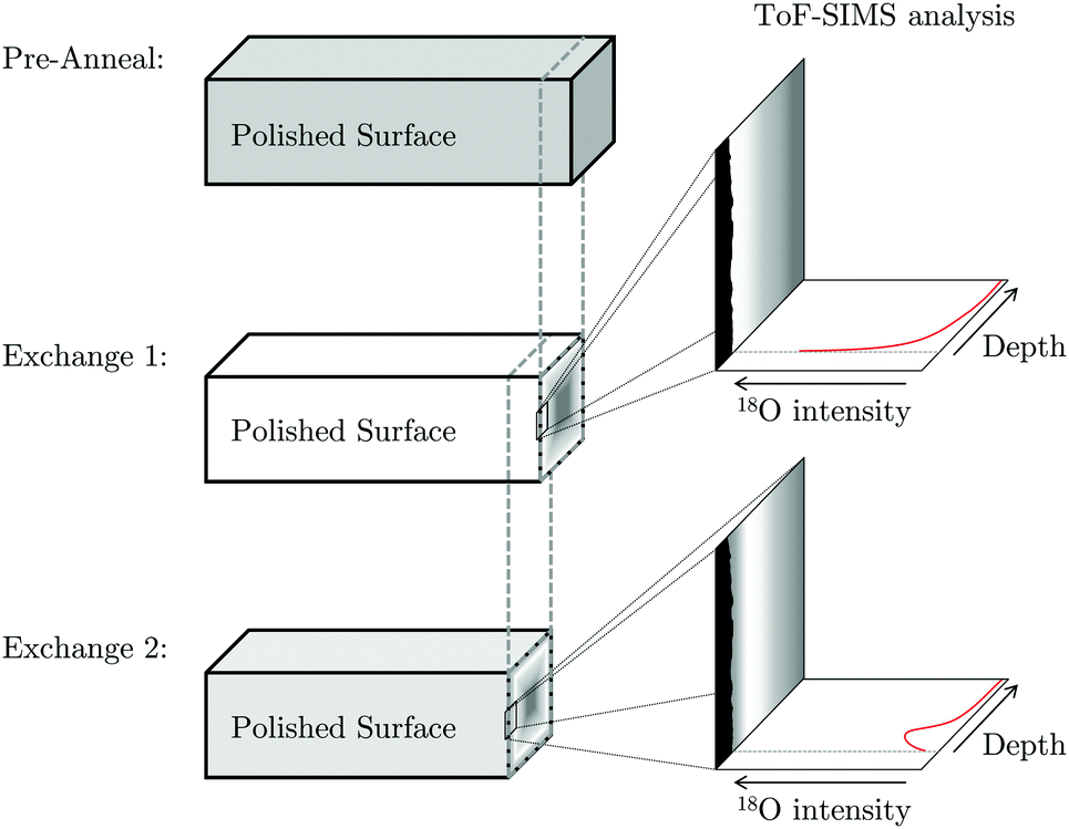 | ||
| Fig. 3 Schematic representation of the progress grinding of the pellet surface between exchanges in order to capture ToF-SIMS images from the cross-section. | ||
The value of Cbg was measured from an unexchanged, but similarly prepared sample using the same imaging method and Cgas was measured during the exchange using the silicon wafer technique described in ref. 12.
3.1 Data processing
Before the 2D images were collapsed into 1D line-scans, some data processing was required to correct for several established sources of error. A Poisson correction is applied to each mass peak to correct for counts missed due to the “dead time” of the detector, as discussed in ref. 13. This correction has a very significant effect in the detection of low isotopic fractions, which is relevant to the accurate measurement of the background concentration of 18O (Cbg ≈ 0.2% = 1/500).Bilinear interpolation was used to produce an image rotation series at 0.1° increments. After generating a profile at each step, it was possible to align the exchange surface by choosing the angle with the maximum gradient of total counts (16O + 18O), this same process was also used to find the location of the “surface”. Typically, however, the degree of misalignment was small (<±2°), which has only a modest effect on the fitted values of D* and k* as long as the surface location is specified as the mean surface, rather than the leading point. Fig. 4 shows the mean oxygen counts (16O + 18O) against distance from the surface, superimposed onto the 2D ToF-SIM image for sample C, which required 1° of clockwise rotational alignment.
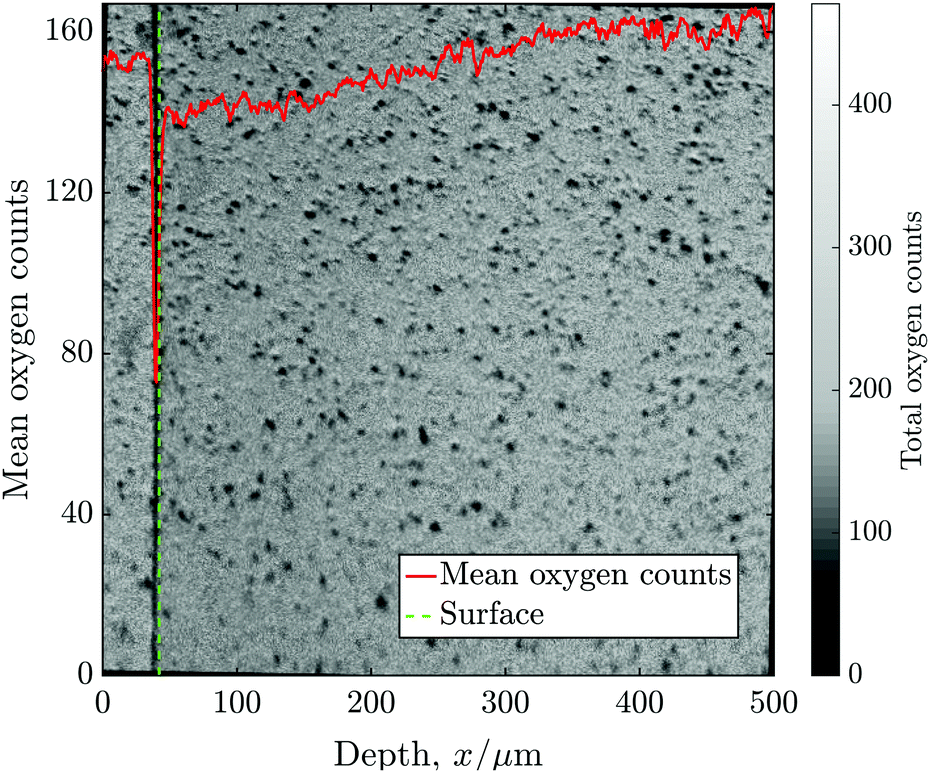 | ||
| Fig. 4 The mean oxygen counts (16O + 18O) against distance from the surface, superimposed onto the 2D ToF-SIM image for sample C. The image shows two samples stuck together and the nominal location of the surface of the sample of interest is also highlighted. | ||
Following alignment, the isotopic fraction was calculated in each pixel and then the mean of each column was used to construct a 1D depth profile. Fig. 5 shows the isotopic fraction (18O/(16O + 18O)) against distance from the surface, superimposed onto the normalised 2D ToF-SIM data.
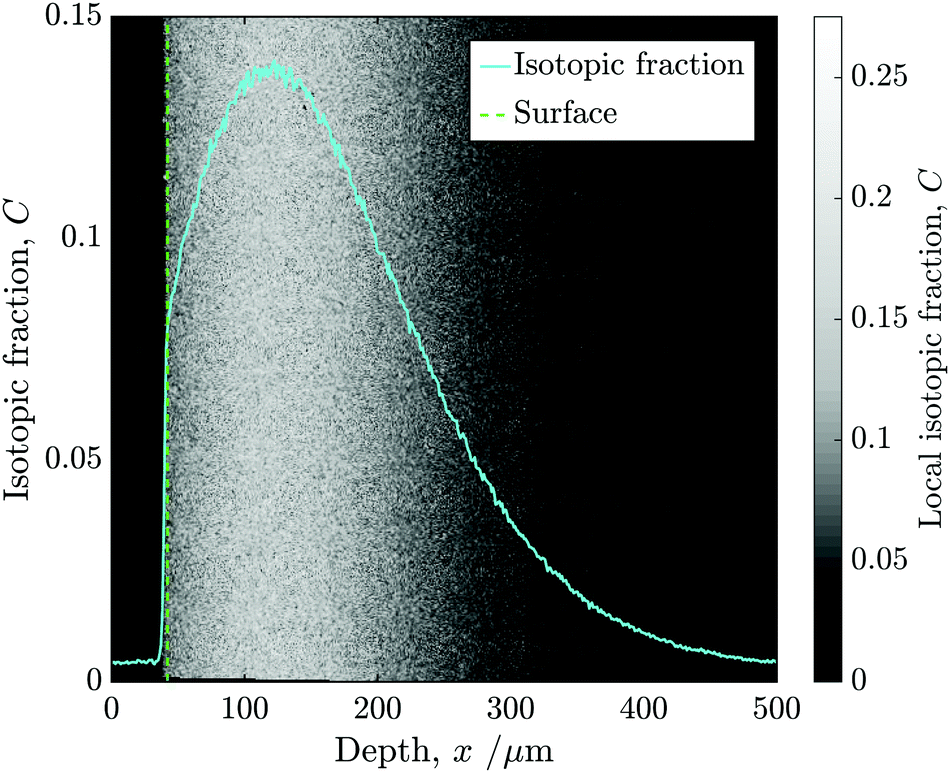 | ||
| Fig. 5 The isotopic fraction (18O/(16O + 18O)) against distance from the surface, superimposed onto the normalised 2D ToF-SIM data. The image show two samples stuck together (one of which has not undergone isotopic exchange) and the nominal location of the surface of the sample of interest is also highlighted. | ||
For each exchange, the time-temperature profile inside the furnace was recorded using a shielded thermocouple. The nominal duration of the first and second exchange steps were 1.5 h and 0.75 h respectively. By analysing the thermocouple data, the effective temperature was set to 785 °C and, using the method described by Killoran,6 the effective exchange times were calculated to be, ϕ1 = 1.4 h and ϕ2 = 0.66 h.
In order to make this correction, the Killoran method requires an activation energy of diffusion for the LSCF6428. The value used here was Ea = 1.917 eV and although this value was itself derived from a similar experiment,14 a sensitivity study suggests the resulting effective anneal times were highly insensitive to its value (<1 min eV−1). A separate activation energy is associated with the surface exchange coefficient, which is more difficult to account for as the surface exchange boundary condition is a function of both D* and k*. However, the rapid heating/cooling rates (c. 170 °C min−1) combined with suitable anneal times (>40 min in all cases) should minimise any resulting discrepancies.
4 Results
Fig. 6 shows the profiles generated from the line-scans for experiments A–C. In each case the vertical axis was normalised using eqn (2).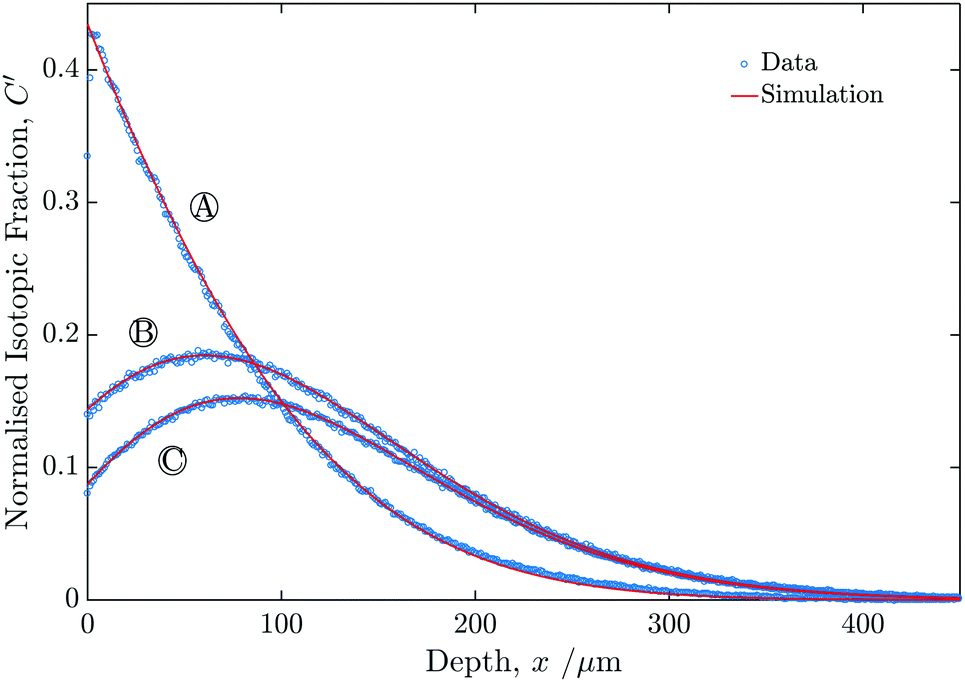 | ||
| Fig. 6 Graph showing the measured isotopic profiles for the three samples (A, B and C), as a function of depth from the sample surface. | ||
The values of k1* extracted from the fits was essentially identical to within reasonable experimental accuracy for all three experiments, as can be seen in Table 1. All three fits had values of R2 above 0.999 measured for the region between the surface and x′ = 2. The value of D* was assumed to be constant for the two exchange steps.
| Sample | D*/10−8 cm2 s−1 | k 1*/10−6 cm s−1 | k 2*/10−6 cm s−1 |
|---|---|---|---|
| A | 1.6 | 1.1 | — |
| B | 1.7 | 1.4 | 1.6 |
| C | 1.7 | 1.3 | 3.3 |
Table 1 also shows that k2* of sample B, was identical to within experimental accuracy to k1* of sample B; whereas k2* of sample C was c. 250% larger than k1* of sample C. Although it is possible to approximate the uncertainty associated with the fitting process, it is expected that this will be small in comparison to other sources, such as sample to sample variation. As such, no uncertainty values are reported. The surface position and the size of the raster step are determined through calibration and contribute both a systematic and a statistical error.
5 Discussion
The results of the three experiments appear to show the validity and the utility of the back-exchange approach both through the consistency of k1* across all samples, as well as the significant variation between the two values of k2*. In all cases, the surface exchange coefficient in pure, dry, isotopically enriched O2 was in excellent agreement both between the experiments and with the literature.15 The surface exchange coefficient for the second exchange in experiment B was also in excellent agreement (to within experimental accuracy) with all values of k1*, which validates the back-exchange procedure. In all of the dry oxygen exchanges, the oxygen used was very high purity (99.999% pure) and measured to be very dry (<1 vpm H2O), which we believe to be crucial in the consistency of the result.There are several possible mechanism for the augmentation of k* in the presence of air compared to dry oxygen. Ambient air contains a wide range of oxygen containing components and it is known that H2O and CO216–18 can both significantly influence the overall oxygen exchange rate. Literature data suggests that both the temperature and overall composition of the anneal environment effects the measured oxygen exchange rate. It was beyond the scope of this paper to quantify the direct effect of each gaseous component; however, it should be clear that the back-exchange technique is capable of making these measurements in a systematic study.
5.1 Experimental error
As can be seen in Table 1 the k1* values have a small degree of variation. The source of this error may potentially be due to microstructural differences between samples. For this experiment, each sample was cut from the same sintered pellet and so assumed to be identical; however, subsurface defects (such as pores) could not be measured. Closed porosity will affect the local transport properties and thus adjust the measured diffusion profile.For a number of common perovskite-based MIEC materials, exsolution of A-site cations to form secondary phase surface particles is a common occurrence.19–22 These particles are typically non-conductive and thus reduce the catalytically active area for the reduction and incorporation of oxygen. It has been shown that significant ‘strontium segregation’ can occur in LSCF6428 at relatively low temperatures and short anneal times.20,22 However, high temperature environmental scanning electron microscopy was used to inspect the surface of the LSCF6428 before and after annealing and no surface particles were observed.
The k1* value of sample B and C show excellent accordance, however, sample A appears to be lower. As mentioned previously, the statistical dead-time corrections are an additional source of error. Using the line-scan method and ToF-SIMS analysis, a constant total ion count is necessary to ensure accurate isotopic fraction measurement; however, the geometry and surface roughness of the sample can alter secondary ion extraction rates. Polishing the surface to a 0.25 μm grade is sufficient to negate these errors across the bulk surface, but at the edge of the sample it is very difficult to prevent curvature during to the polishing process. The radius of curvature (and thus number of affected pixels in the 2D ion image) determines surface uncertainty of the profile. In this work samples were adhered together prior to the second polishing step using a commercially available epoxy resin. This minimised the curvature to approximately 1 μm to 2 μm, greatly reducing the uncertainty of the line-scan profile near the surface.
5.2 Profile uncertainty
Fig. 7 is essentially a section through Fig. 1 at the time ratio measured in experiment C (θ = 0.47), although the vertical axis was left as C′ rather than C*. A family of profiles were generate by varying λ by a factor of 2 between each.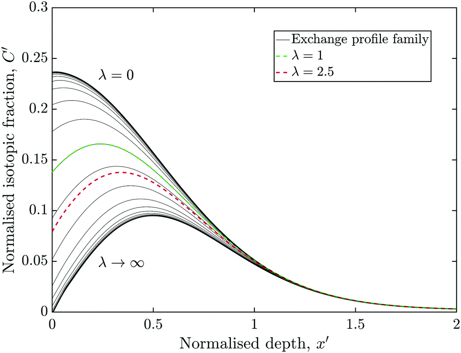 | ||
| Fig. 7 The family of possible profiles for the exchange conditions of experiment C (θ = 0.47), assuming D1* = D2*. The experimentally derived profile is shown in red and the case of where k2* = k1* (λ = 1) is highlighted in green. | ||
The red curve highlights the case where λ = 1 (i.e. k2* = k1*), which was close to the measured result of experiment B. The green curve is where k2* = 2.5 × k1*, similar to experiment C. For very small or very large value of λ, the profiles approach an asymptote, which would undermine the techniques ability to accurately measure the corresponding values of k2*.
When D1* and D2* were allowed to float independently during the fitting, a family of similar curves could be generated, which all closely fit the profile. However, all samples tested were sections cut from the same pellet and also exchanged for identical times and temperatures, thus making it reasonable to assume that the profiles generated in the first exchange was the same for experiments A–C. This suggests that, for the back-exchange fitting, profiles where D1* and k1* are close to that resulting from experiment A should be preferred.
All of the data analysis, curve fitting and graphs were generated using a custom software package, TraceX,23 which is a GUI developed using the MatLab guide platform. The latest version of TraceX is freely available from the supplementary materials section of this publication and those interested are encouraged to contact the author.
6 Conclusions
A novel back-exchange technique has been developed to quantify the effect of contaminants on the effective surface exchange coefficient. This involves a two-step exchange process, followed by line-scan SIMS imaging of the isotopic fraction. A new analytical solution was derived for a special case of this system and a Crank-Nicholson type finite difference simulation was used where it could not be applied (i.e. where k2* ≠ k1*). The technique was validated by comparison with values derived from a conventional exchange profile as well as values from the literature. This work found that ambient air had caused a c. 250% increase in the value of k* compared to pure, dry O2, which demonstrates the significance of the technique. The back-exchange approach can also be extended to any atmosphere with the same pO2 as that of the first exchange step; however, care must be taken when approaching the asymptotic regions of the profiles as uncertainty can become large and asymmetric. Further work must be done to isolate the effect of each gas component in air.Acknowledgements
The authors would like to thank Dr Richard Chater and Dr Sarah Fearn of Imperial College London for the guidance with the ToF-SIMS analysis, as well as Dr Renaud Podor of the L'Institut de Chimie Séparative de Marcoule (ICSM) for his work on the HT-ESEM. The authors would also like to acknowledge the EPSRC grant EP/J003085/1 for supporting this work.References
- J. A. Kilner, B. Steele and L. Ilkov, Solid State Ionics, 1984, 12, 89–97 CrossRef CAS.
- R. Chater, S. Carter, J. Kilner and B. Steele, Solid State Ionics, 1992, 53–56, 859–867 CrossRef CAS.
- R. A. De Souza, J. Zehnpfenning, M. Martin and J. Maier, Solid State Ionics, 2005, 176, 1465–1471 CrossRef CAS.
- H. S. Carslaw and J. C. Jaeger, J. Mech. Phys. Solids, 1959, XXXIII, 81–87 Search PubMed.
- J. Crank, The Mathematics of Diffusion, Clarendon press, Oxford, 1975, vol. 2 Search PubMed.
- D. Killoran, J. Electrochem. Soc., 1962, 109, 170–171 CrossRef.
- H. Brezis, Analyse fonctionnelle. Théorie et applications, Masson, Paris, France, 1983 Search PubMed.
- J. Crank and P. Nicolson, Proc. Cambridge Philos. Soc., 1947, 43, 50–67 CrossRef.
- J. W. Thomas, Numerical Partial Differential Equations: Finite Difference Methods, Springer Science & Business Media, 1995, vol. 22 Search PubMed.
- J. Nelder and R. Mead, Comput. J., 1965, 7, 308–313 CrossRef.
- N. J. Higham, The Matrix Computation Toolbox for MATLAB (Version 1.0), Manchester Centre for Computational Mathematics, 2002, p. 19 Search PubMed.
- R. J. Chater, PhD thesis, Imperial College London, 2014.
- T. Stephan, J. Vac. Sci. Technol., A, 1994, 12, 405–410 CAS.
- S. J. Benson, PhD thesis, Imperial College London, 1999.
- Y. Li, K. Gerdes, T. Horita and X. Liu, J. Electrochem. Soc., 2013, 160, F343–F350 CrossRef CAS.
- N. Sakai, K. Yamaji, T. Horita, Y. P. Xiong, H. Kishimoto and H. Yokokawa, J. Electrochem. Soc., 2003, 150, A689 CrossRef CAS.
- S. J. Benson, D. Waller and J. A. Kilner, J. Electrochem. Soc., 1999, 146, 1305 CrossRef CAS.
- S. Darvish, M. Asadikiya, B. Hu, P. Singh and Y. Zhong, Int. J. Hydrogen Energy, 2016, 41, 10239–10248 CrossRef CAS.
- M. Finsterbusch, A. Lussier, J. A. Schaefer and Y. U. Idzerda, Solid State Ionics, 2012, 212, 77–80 CrossRef CAS.
- D. Oh, D. Gostovic and E. D. Wachsman, J. Mater. Res., 2012, 27, 1992–1999 CrossRef CAS.
- Y. Chen, H. Téllez, M. Burriel, F. Yang, N. Tsvetkov, Z. Cai, D. W. McComb, J. A. Kilner and B. Yildiz, Chem. Mater., 2015, 27, 5436–5450 CrossRef CAS.
- J. Druce, T. Ishihara and J. A. Kilner, Solid State Ionics, 2014, 262, 893–896 CrossRef CAS.
- S. J. Cooper, PhD thesis, Imperial College London, 2015.
| This journal is © the Owner Societies 2017 |