
 Open Access Article
 This Open Access Article is licensed under a
 Creative Commons Attribution 3.0 Unported Licence
Energy landscapes for machine learning
Andrew J.
Ballard
a,
Ritankar
Das
a,
Stefano
Martiniani
 a,
Dhagash
Mehta
b,
Levent
Sagun
c,
Jacob D.
Stevenson
d and
David J.
Wales
*a
a,
Dhagash
Mehta
b,
Levent
Sagun
c,
Jacob D.
Stevenson
d and
David J.
Wales
*a
aUniversity Chemical Laboratories, Lensfield Road, Cambridge CB2 1EW, UK. E-mail: dw34@cam.ac.uk
bDepartment of Applied and Computational Mathematics and Statistics, University of Notre Dame, IN, USA
cMathematics Department, Courant Institute, New York University, NY, USA
dMicrosoft Research Ltd, 21 Station Road, Cambridge, CB1 2FB, UK
First published on 3rd April 2017
Abstract
Machine learning techniques are being increasingly used as flexible non-linear fitting and prediction tools in the physical sciences. Fitting functions that exhibit multiple solutions as local minima can be analysed in terms of the corresponding machine learning landscape. Methods to explore and visualise molecular potential energy landscapes can be applied to these machine learning landscapes to gain new insight into the solution space involved in training and the nature of the corresponding predictions. In particular, we can define quantities analogous to molecular structure, thermodynamics, and kinetics, and relate these emergent properties to the structure of the underlying landscape. This Perspective aims to describe these analogies with examples from recent applications, and suggest avenues for new interdisciplinary research.
I. Introduction
Optimisation problems abound in computational science and technology. From force field development to thermodynamic sampling, bioinformatics and computational biology, optimisation methods are a crucial ingredient of most scientific disciplines.1 Geometry optimisation is a key component of the potential energy landscapes approach in molecular science, where emergent properties are predicted from local minima and the transition states that connect them.2,3 This formalism has been applied to a wide variety of physical systems, including atomic and molecular clusters, biomolecules, mesoscopic models, and glasses, to understand their structural properties, thermodynamics and kinetics. The methods involved in the computational potential energy landscapes approach amount to optimisation of a non-linear function (energy) in a high-dimensional space (configuration space). Machine learning problems employ similar concepts: the training of a model is performed by optimising a cost function with respect to a set of adjustable parameters.Understanding how emergent observable properties of molecules and condensed matter are encoded in the underlying potential energy surface is a key motivation in developing the theoretical and computational aspects of energy landscape research. The fundamental insight that results has helped to unify our understanding of how structure-seeking systems, such as ‘magic number’ clusters, functional biomolecules, crystals and self-assembling structures, differ from amorphous materials and landscapes that exhibit broken ergodicity.3–6 Rational design of new molecules and materials can exploit this insight, for example associating landscapes for self-assembly with a well defined free energy minimum that is kinetically accessible over a wide range of temperature. This structure, where there are no competing morphologies separated from the target by high barriers, corresponds to an ‘unfrustrated’ landscape.2,5,7,8 In contrast, designs for multifunctional systems, including molecules with the capacity to act as switches, correspond to multifunnel landscapes.9,10
In this Perspective we illustrate how the principles and tools of the potential energy landscape approach can be applied to machine learning (ML) landscapes. Some initial results are presented, which indicate how this view may yield new insight into ML training and prediction in the future. We hope our results will be relevant for both the energy landscapes and machine learning communities. In particular, it is of fundamental interest to compare these ML landscapes to those that arise for molecules and condensed matter. The ML landscape provides both a means to visualise and interpret the cost function solution space and a computational framework for quantitative comparison of solutions.
II. The energy landscape perspective
The potential energy function in molecular science is a surface defined in a (possibly very high-dimensional) configuration space, which represents all possible atomic configurations.2,11 In the potential energy landscape approach, this surface is divided into basins of attraction, each defined by the steepest-descent pathways that lead to a particular local minimum.2,11 The mapping from a continuous multidimensional surface to local minima can be very useful. In particular, it provides a route to prediction of structure and thermodynamics.2 Similarly, transitions between basins can be characterised by geometric transition states (saddle points of index one), which lie on the boundary between one basin and another.2 Including these transition states in our description of the landscape produces a kinetic transition network,3,12,13 and access to dynamical properties and ‘rare’ events.14–17 The pathways mediated by these transition states correspond to processes such as molecular rearrangements, or atomic migration. For an ML landscape we can define the connectivity between minima that represent different locally optimal fits to training data in an analogous fashion. To the best of our knowledge, interpreting the analogue of a molecular rearrangement mechanism for the ML landscape has yet to be explored.Construction of a kinetic transition network3,12,13 also provides a convenient means to visualise a high-dimensional surface. Disconnectivity graphs4,18 represent the landscape in terms of local minima and connected transition states, reflecting the barriers and topology through basin connectivity. The overall structure of the disconnectivity graph can provide immediate insight into observable properties:4 a single-funnelled landscape typically represents a structure-seeking system that equilibrates rapidly, whereas multiple funnels indicate competing structures or morphologies, which may be manifested as phase transitions and even glassy phenomenology. Locating the global minimum is typically much easier for single funnel landscapes.19
The decomposition of a surface into minima and transition states is quite general and can naturally be applied to systems that do not correspond to an underlying molecular model. In particular, we can use this strategy for machine learning applications, where training a model amounts to minimisation of a cost function with respect to a set of parameters. In the language of energy landscapes, the machine learning cost function plays the role of energy, and the model parameters are the ‘coordinates’ of the landscape. The minimised structures represent the optimised model parameters for different training iterations. The transition states are the index one saddle points of the landscape.20
Energy landscape methods2 could be particularly beneficial to the ML community, where non-convex optimisation has sometimes been viewed as less appealing, despite supporting richer models with superior scalability.21 The techniques described below could provide a useful computational framework for exploring and visualising ML landscapes, and at the very least, an alternative view to non-convex optimisation. The first steps in this direction have recently been reported.22–24 The results may prove to be useful for various applications of machine learning in the physical sciences. Examples include fitting potential energy surfaces, where neural networks have been used extensively25–32 for at least 20 years.33–35 Recent work includes prediction of binding affinities in protein–ligand complexes,36 applications to the design of novel materials,37,38 and refinement of transition states39 using support vector machines.40
In the present contribution we illustrate the use of techniques from the energy landscapes field to several ML examples, including non-linear regression, and neural network classification. When surveying the cost function landscapes, we employed the same techniques and algorithms as for the molecular and condensed matter systems of interest in the physical sciences: specifically, local and global minima were obtained with the basin-hopping method41–43 using a customised LBFGS minimisation algorithm.44 Transition state searches employed the doubly-nudged45,46 elastic band47,48 approach and hybrid eigenvector-following.49,50 These methods are all well established, and will not be described in detail here. We used the python-based energy landscape explorer pele,51 with a customised interface for ML systems, along with the GMIN,52 OPTIM,53 and PATHSAMPLE54 programs, available for download under the Gnu General Public Licence.
III. Prediction for classification of outcomes in local minimisation
Neural networks (NN) have been employed in two previous classification problems that analyse the underlying ML landscape, namely predicting which isomer results from a molecular geometry optimisation23 and for patient outcomes in a medical diagnostic context.24 Some of the results from the former study will be illustrated here, and we must carefully distinguish isomers corresponding to minima of a molecular potential energy landscape from the ML landscape of solutions involved in predicting which of the isomers will result from geometry optimisation starting from a given molecular configuration. We must also distinguish this classification problem from ab initio structure prediction: the possible outcomes of the geometry optimisation must be known in advance, either in terms of distinct isomers, or the range that they span in terms of potential energy or appropriate structural order parameters for larger systems. The ability to make predictions that are sufficiently reliable could produce significant savings in computational effort for applications that require repeated local minimisation. Examples include basin-sampling for calculating global thermodynamic properties in systems subject to broken ergodicity,55 construction of kinetic transition networks,56 and methods to estimate the volume of basins of attraction for jammed packings, which provide measures of configurational entropy in granular packings.57 Here the objective would be to terminate the local minimisation as soon as the outcome could be predicted with sufficient confidence to converge the properties of interest.23,58The test system considered here is a simple triatomic cluster with four distinguishable local minima that represent the possible outcomes for local minimisation. This system has previously served as a benchmark for visualising the performance of different geometry optimisation approaches.59–61 The potential energy, V, is a sum of pairwise terms, corresponding to the Lennard-Jones form,62 and the three-body Axilrod–Teller function,63 which represents an instantaneous induced dipole–induced dipole interaction:
 | (1) |
The objective of our machine learning calculations for this system is a classification, to predict which of the four minima a local minimisation would converge to, given data for one or more configurations. The data in question could be combinations of the energy, gradient, and geometrical parameters for the structures in the optimisation sequence. Our initial tests, which are mostly concerned with the structure of the ML solution landscape, employed the three interparticle separations r12, r13 and r23 as data.23 Inputs were considered for separations corresponding to the initial geometry, and for one or more configurations in the minimisation sequence.
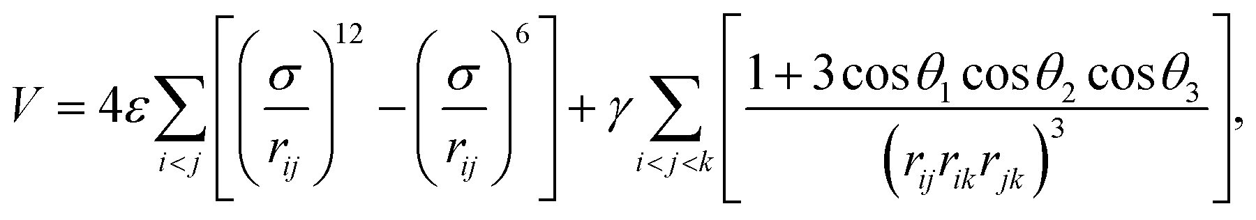
A database of 10![[thin space (1/6-em)]](https://www.rsc.org/images/entities/char_2009.gif) 000 energy minimisations, each initiated from different atomic coordinates distributed in a cube of side length
000 energy minimisations, each initiated from different atomic coordinates distributed in a cube of side length  , was created using the customised LBFGS routine in our OPTIM program53 (LBFGS is a limited memory quasi-Newton Broyden,64 Fletcher,65 Goldfarb,66 Shanno,67 scheme). Each minimisation was converged until the root mean square gradient fell below 10−6 reduced units, and the outcome (one of the four minima) was recorded.
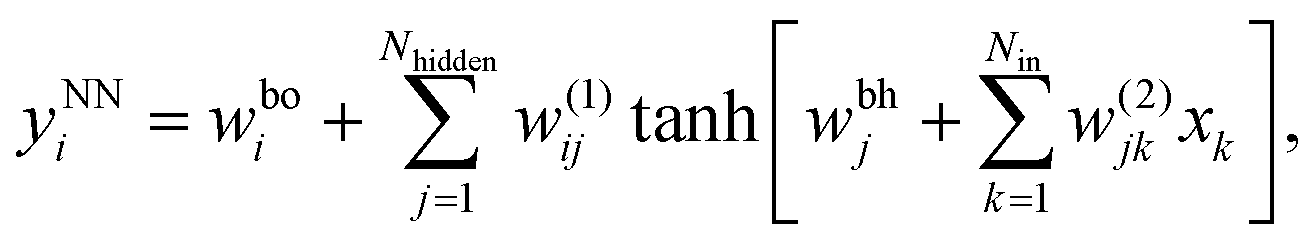
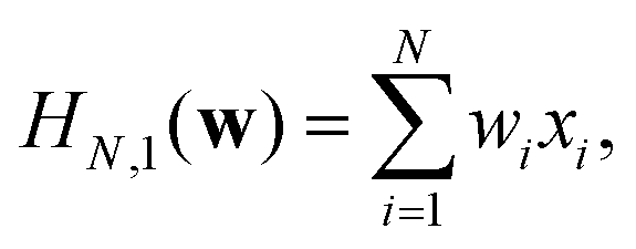
The neural networks used in the applications discussed below all have three layers, corresponding to input, output, and hidden nodes.68 A single hidden layer has been used successfully in a variety of previous applications.69 A bias was added to the sum of weights used in the activation function for each hidden node, wbhj, and each output node, wboi, as illustrated in Fig. 1. For inputs we consider X = {x1,…,xNdata}, where Ndata is the number of minimisation sequences in the training or test set, each of which has dimension Nin, so that  . For this example there are four outputs corresponding to the four possible local minima (as in Fig. 1), denoted by yNNi, with
 | (2) |
 | ||
| Fig. 1 Organisation of a three-layer neural network with three inputs, five hidden nodes, and four outputs. The training variables are the link weights, w(2)jk, w(1)ij, and the bias weights, wbhj and wboi. | ||
The four outputs were converted into softmax probabilities as
 | (3) |
In each training phase we minimise the cost (objective) function, ENN(W;X), with respect to the variables w(1)ij, w(2)jk, wbhj and wboi, which are collected into the vector of weights W. An L2 regularisation term is included in ENN(W;X), corresponding to a sum of squares of the independent variables, multiplied by a constant coefficient λ, which is chosen in advance and fixed. This term is intended to prevent overfitting; it disfavours large values for individual variables. We have considered applications where the regularisation is applied to all the variables, and compared the results with a sum that excludes the bias weights. Regularising over all the variables has the advantage of eliminating the zero Hessian eigenvalue that otherwise results from an additive shift in all the wboi. Such zero eigenvalues are a consequence of continuous symmetries in the cost function (Noether's theorem). For molecular systems such modes commonly arise from overall translation and rotation, and are routinely dealt with by eigenvalue shifting or projection using the known analytical forms for the eigenvectors.2,70 Larger values of the parameter λ simplify the landscape, reducing the number of minima. This result corresponds directly with the effect of compression for a molecular system,71 which has been exploited to accelerate global optimisation. A related hypersurface deformation approach has been used to treat graph partitioning problems.72
For each LBFGS geometry optimisation sequence, d, with Nin inputs collected into data item xd, we know the actual outcome or class label, c(d) = 0, 1, 2 or 3, corresponding to the local minimum at convergence. The networks were trained using either 500 or 5000 of the LBFGS sequences, chosen at random with no overlap, by minimising
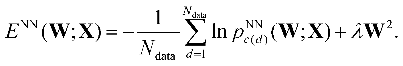 | (4) |
In the testing phase the variables W are fixed for a particular local minimum of ENN(W;Xtrain) obtained with the training data, and we evaluate ENN(W;Xtest) for 500 or 5000 of the minimisation sequences outside the training set. The results did not change significantly between the larger and smaller training and testing sets.
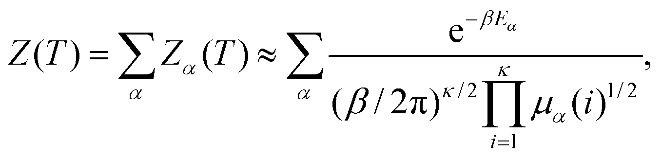
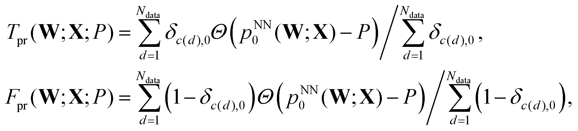
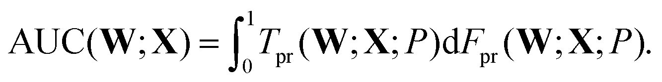
We first summarise some results for ML landscapes corresponding to input data for the three interparticle distances at each initial random starting point. The number of local minima obtained23 was 162, 2559, 4752 and 19045 for three, four, five and six hidden nodes, respectively, with 1504, 10112, 18779 and 34052 transition states. The four disconnectivity graphs are shown in Fig. 2. In each case the vertical axis corresponds to ENN(W;Xtrain), and branches terminate at the values for particular local minima. At a regular series of thresholds for ENN we perform a superbasin analysis,18 which segregates the ML solutions into disjoint sets. Local minima that can interconvert via a pathway where the highest transition state lies below the threshold are in the same superbasin. The branches corresponding to different sets or individual minima merge at the threshold energy where they first belong to a common superbasin. In this case we have coloured the branches according to the misclassification index, discussed further in Section V, which is defined as the fraction of test set images that are misclassified by the minimum in question or the global minimum, but not both. All the low-lying minima exhibit small values, meaning that they perform much like the global minimum. The index rises to between 0.2 and 0.4 for local minima with higher values of ENN(W;Xtrain). These calculations were performed using the pele51 ML interface for the formulation in eqn (2), where regularisation excluded the weights for the bias nodes.23
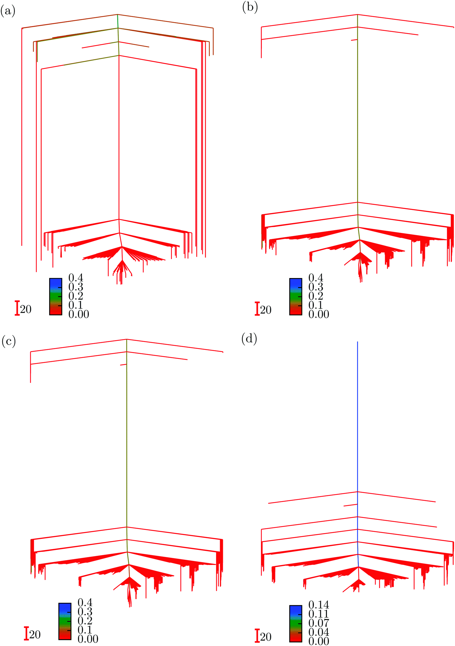 | ||
| Fig. 2 Disconnectivity graphs for the fitting landscapes of a triatomic cluster. Three inputs were used for each minimisation sequence, corresponding to the three interatomic distances in the initial configuration. These graphs are for neural networks with (a) 3, (b) 4, (c) 5, and (d) 6 hidden nodes. The branches are coloured according to the misclassification distance for the local minima evaluated using training data, as described in Section V. | ||
When more hidden nodes are included the dimensionality of the ML landscape increases, along with the number of local minima and transition states. This observation is in line with well known results for molecular systems: as the number of atoms and configurational degrees of freedom increases the number of minima and transition states increases exponentially.73,74 The residual error reported by ENN(W;Xtrain) decreases as more parameters are included, and so there is a trade-off between the complexity of the landscape and the quality of the fit.23
The opportunities for exploiting tools from the potential energy landscape framework have yet to be investigated systematically. As an indication of the properties that might be of interest we now illustrate a thermodynamic analogue corresponding to the heat capacity, CV. Peaks in CV are particularly insightful, and in molecular systems they correspond to phase-like transitions. Around the transition temperature the occupation probability shifts between local minima with qualitatively different properties in terms of energy and entropy: larger peaks correspond to greater differences.75 For the ML landscape we would interpret such features in terms of fitting solutions with different properties. Understanding how and why the fits differ could be useful in combining solutions to produce better predictions. Here we simply illustrate some representative results, which suggest that ML landscapes may support an even wider range of behaviour than molecular systems.
To calculate the CV analogue we use the superposition approach2,73,76–79 where the total partition function, Z(T), is written as a sum over the partition functions Zα(T), for all the local minima, α. This formulation can be formally exact, but is usually applied in the harmonic approximation using normal mode analysis to represent the vibrational density of states. The normal mode frequencies are then related to the eigenvalues of the Hessian (second derivative) matrix, μα(i), for local minimum α:
 | (5) |
lnZ(T)/∂β2.
Many molecular and condensed matter systems exhibit a CV peak corresponding to a first order-like melting transition, where the occupation probability shifts from a relatively small number of low energy minima, to a much larger, entropically favoured, set of higher energy structures, which are often more disordered. However, low temperature peaks below the melting temperature, corresponding to solid–solid transitions, can also occur. These features are particularly interesting, because they suggest the presence of competing low energy morphologies, which may represent a challenge for structure prediction,80 and lead to broken ergodicity,55,79,81–86 and slow interconversion rates that constitute ‘rare events’.14,87,88 Initial surveys of the CV analogue for ML landscapes, calculated using analytical second derivatives of ENN(Wα;X), produced plots with multiple peaks, suggesting richer behaviour than for molecular systems.
One example is shown in Fig. 3, which is based on the ML solution landscape for a neural network with three hidden nodes and inputs corresponding to the three interparticle distances at the initial geometries of all the training optimisation sequences. These results were obtained using the pele51 ML interface for the neural network formulation in eqn (2), where regularisation did not include the weights for the bias nodes.23 The superposition approach provides a clear interpretation for the peaks, which we achieve by calculating CV from partial sums over the ML training minima, in order of increasing ENN(Wα;Xtrain). The first peak around kBT ≈ 0.2 arises from competition between the lowest two minima. The second peak around kBT ≈ 9 is reproduced when the lowest 124 minima are included, and the largest peak around kBT ≈ 20 appears when we sum up to minimum 153. The latter solution exhibits one particularly small Hessian eigenvalue, producing a relatively large configurational entropy contribution, which increases with T. The harmonic approximation will break down here, but nevertheless serves to highlight the qualitative difference in character of minima with exceptionally small curvatures.
 | ||
| Fig. 3 Heat capacity analogue for the ML landscape defined for the dataset using only the three initial interatomic distances with three hidden nodes. The insets illustrate the convergence of the two low temperature peaks. In each plot the black curve corresponds to CV calculated from the complete database of minima. The red curves labelled ‘2’, ‘124’ and ‘152’ correspond to CV calculated from truncated sums including only the lowest 2, 124, and 152 minima, respectively. | ||
In molecular systems competition between alternative low energy structures often accounts for CV peaks corresponding to solid–solid transitions, and analogues of this situation may well exist in the ML scenario. Some systematic shifts in the CV analogue could result from the density of local minima on the ML landscape (the landscape entropy89–92). Understanding such effects might help to guide the construction of improved predictive tools from combinations of fitting solutions. Interpreting the ML analogues of molecular structure and interconversion rates between minima might also prove to be insightful in future work.
A subsequent study investigated the quality of the predictions using two of the three interatomic distances, r12 and r13, and the effects of memory, in terms of input data from successive configurations chosen systematically from each geometry optimisation sequence.93 The same database of LBFGS minimisation sequences for the triatomic cluster was used here, divided randomly into training and testing sets of equal size (5000 sequences each). The quality of the classification prediction into the four possible outcomes can be quantified using the area under curve (AUC) for receiver operating characteristic (ROC) plots.69 ROC analysis began when radar receiver operators needed to distinguish signals corresponding to aircraft from false readings, including flocks of birds. The curves are plots of the true positive rate, Tpr, against the false positive rate, Fpr, as a function of the threshold probability, P, for making a certain classification. Here, P is the threshold at which the output probability pNN0(W;X) is judged sufficient to predict that a minimisation would converge to the equilateral triangle, so that
 | (6) |
 | (7) |
Fig. 4 shows the AUC values obtained with the LBFGS database when the input data consists of r12 and r13 values at different points in the minimisation sequence. Here the horizontal axis corresponds to s, the number of steps from convergence, and the AUC values therefore tend to unity when s is small, where the configurations are close to the final minimum. Each panel in the figure includes two plots, which generally coincide quite closely. The plot with the lower AUC value is the one obtained with the global minimum located for ENN(Wα;Xtrain) for configurations s steps for convergence. The AUC value in the other plot is always greater than or equal to the value for the global minimum, since it is the maximum AUC calculated for all the local minima characterised with the same neural net architecture and any s value. Minimisation sequences that converge in fewer than s steps are padded with the initial configuration for larger s values, which is intended to present a worst case scenario.
 | ||
| Fig. 4 AUC values for 5000 minimisation sequences in the LBFGS testing set, evaluated using the parameters obtained for the global minimum neural network fit with 5000 training sequences and λ = 10−4. The four panels correspond to 3, 4, 5 or 6 hidden nodes, as marked, and the lower curve corresponds to the global minimum of ENN(Wα;Xtrain) with Xtrain containing r12 and r13 at a single configuration in each minimisation sequence, located s steps from convergence. Each panel has a second plot of the highest AUC value for the test data attained with any local minimum obtained in training having the same number of inputs and hidden nodes, including results for all the λ values considered and for all values of s, from 1 to 80. The AUC value for the global minimum with λ = 10−4 and the configuration in question is included in this set, but can be exceeded by one of the many local minima obtained over the full range of λ and s. Beyond s around 60 the plots are essentially flat. | ||
Fig. 4 shows that the prediction quality decays in a characteristic fashion as configurations move further from the convergence limit. It also illustrates an important result, namely that the performance of the global minimum obtained with the training data is never surpassed significantly by any of the other local minima, when all these fits are applied to the test data. Hence the global minimum is clearly a good place to start if we wish to make predictions, or perhaps construct classification schemes based on more than one local minimum of the ML landscape obtained in training. The corresponding fits and AUC calculations were all rerun to produce Fig. 4 using the fitting function defined in eqn (2) and regularisation over all variables, for comparison with the simplified bias weighting employed in ref. 93. There is no significant difference between our results for the two schemes.
IV. Non-linear regression
Regression is perhaps the most well-known task in machine learning, referring to any process for estimating the relationships between dependent and independent variables. As we show in this section, even a relatively simple non-nonlinear regression problem leads to a rich ML landscape. As in the standard regression scenario, we consider a set of Ndata data points D = ((x1,t1),…,(xNdata,tNdata)), and a model y(x;q) that we wish to fit to D by adjusting M parameters q = (q1,q2,…,qM). In this example, we investigate the following non-linear model:| y(x;q) = e−q1xsin(q2x + q3)sin(q4x + q5). | (8) |
We performed regression on the above problem, with a dataset D consisting of Ndata = 100 data points with xi values sampled uniformly in [0,3π], and corresponding ti values given by our model with added Gaussian white noise (mean zero, σ = 0.02):
| ti = y(xi;q*) + noise, | (9) |
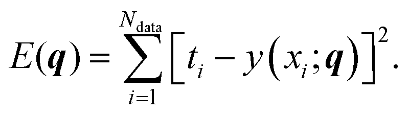 | (10) |
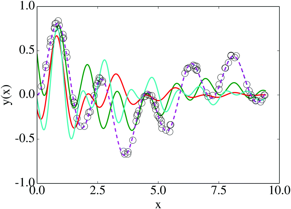
We explored the landscape described by E(q), and display the various solutions in Fig. 5 alongside our data and y(x;q = q*). In this case, the global minimum is a fairly accurate representation of the solution used to generate D. However, 88 other solutions were found which do not accurately represent the data, despite being valid local minima. In Fig. 6 we show the disconnectivity graph for E(q). Here the vertical axis corresponds to E(q), and branches terminate at the values for corresponding local minima, as in Section III. The graph shows that the energy of the global minimum solution is separated from the others by an order of magnitude, and is clearly the best fit to our data (dotted curve in Fig. 5). The barriers in this representation can be interpreted in terms of transformations between different training solutions in parameter space, and could be indicative of the distinctiveness of the minima they connect. The minima of this landscape were found by the basin-hopping method,41–43 as described in Section II.
 | ||
| Fig. 5 Results from nonlinear regression for the model given by eqn (8): the global minimum of the cost function (dashed line) is plotted with various local minima solutions (solid lines) and the data used for fitting (black circles). The model used to generate the data is indistinguishable from the curve corresponding to the global minimum. | ||
 | ||
| Fig. 6 Disconnectivity graph for a nonlinear regression cost function [eqn (8)]. Each branch terminates at a local minimum at the value of E(q) for that minimum. By following the lines from one minimum to another, one can read off the energy barrier on the minimum energy path connecting them. | ||
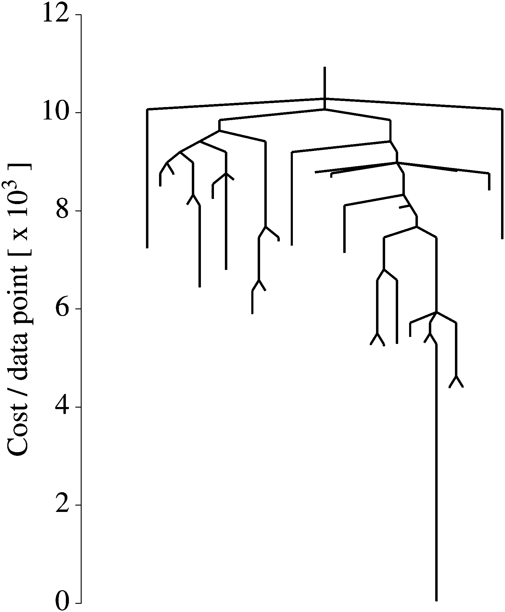
V. Digit recognition using a neural network
The next machine learning landscape we explore here is another artificial neural network, this time trained for digit recognition on the MNIST dataset.94 Our network architecture consists of 28 × 28 input nodes corresponding to input image pixels, a single hidden layer with 10 nodes, and a softmax output layer of 10 nodes, which represent the 10 digit classes. This model contains roughly 8000 adjustable parameters, which quantify the weight of given nodes in activating one of their successors. The cost function we optimise for this classification example is the same multinomial logistic regression function that is described above in Section III, which is standard for classification problems. Here ‘logistic’ means that the dependent variable (outcome) is a category, in this case the assignment of the image for a digit, and ‘multinomial’ means that there are more than two possible outcomes. An L2 regularisation term was again added to the cost function, as described in Section III. Unless otherwise mentioned, all the results described below are for a regularisation coefficient of λ = 0.1.The neural network defined above is quite small, and is not intended to compete with well-established models trained on MNIST.95 Rather, our goal in this Perspective is to gain insight into the landscape. This aim is greatly assisted by using a model that is smaller, yet still behaves similarly to more sophisticated implementations. To converge the disconnectivity graph, Fig. 7, in particular the transition states, the model was trained on Ndata = 1000 data points. The results assessing performance, Fig. 8 and 9, were tested on Ndata = 10000 images.
 | ||
| Fig. 7 Disconnectivity graph of neural network ML solutions for digit recognition. | ||
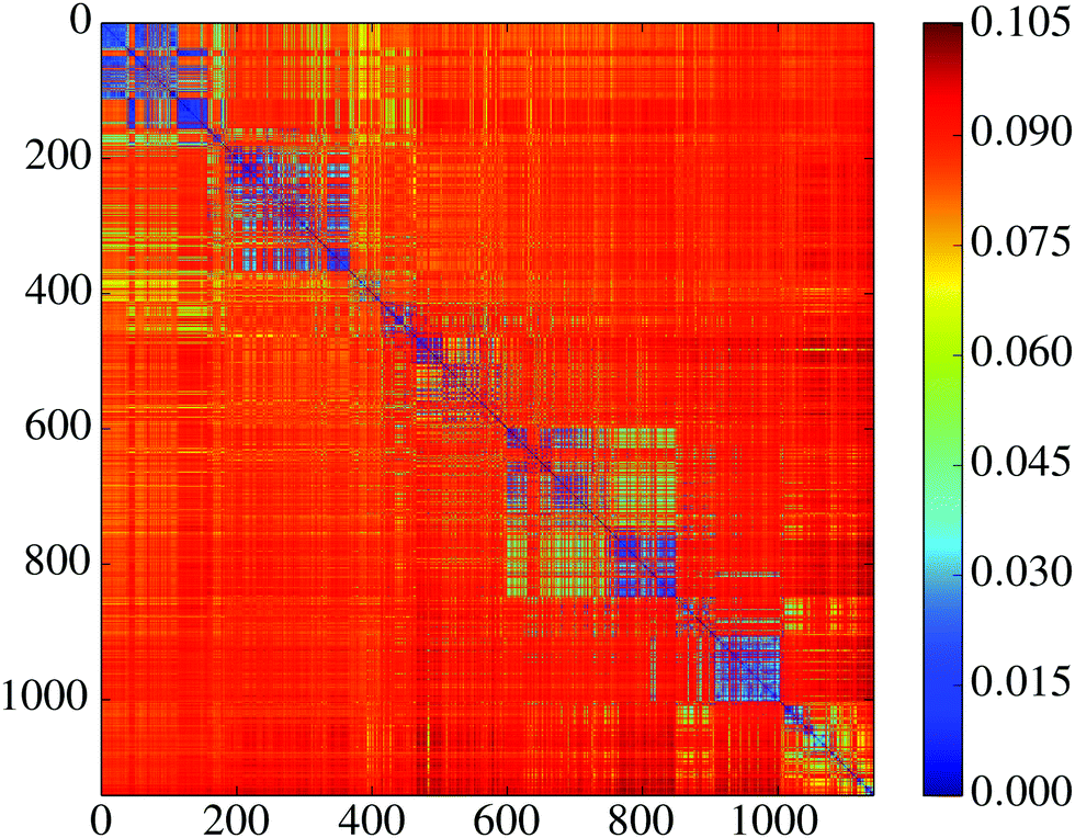 | ||
| Fig. 8 Misclassification heat map for various solutions to the digit recognition problem on the ML landscape. This map displays the degree of similarity of any pair of minima based upon correct test set classification. See text for details. | ||
 | ||
| Fig. 9 Joint probability density plot of minimum–minimum Hamming distance and geometric distance in parameter space. The distance metric in parameter space is correlated with the misclassification distance between minima. The probability density is coloured on a log scale. | ||
We explored the landscape of this network for several different values of the L2 regularisation parameter λ. The graph shown in Fig. 7, with λ = 0.01, is representative of all the others: we observe a single funnel landscape, where, in contrast to the nonlinear regression example, all of the minima occur in a narrow range of energy (cost) values. This observation is consistent with recent work suggesting that the energies of local minima for neural networks are spaced exponentially close to the global minimum96,97 with the number of variables (number of optimised parameters or dimensionality) of the system.
We next assess the performance profile of the NN minima by calculating the misclassification rate on an independent test set. Judging by average statistics the minima seem to perform very similarly: the fraction f of misclassified test set images is comparable for most of them, with 0.133 ≤ f ≤ 0.162 (mean ![[f with combining macron]](https://www.rsc.org/images/entities/i_char_0066_0304.gif) = 0.148, standard deviation σf = 0.0043). This observation is also consistent with previous results where local minima were found to perform quite similarly in terms of test set error.98,99 When looking beyond average statistics, however, we uncover more interesting behaviour. To this end we introduce a misclassification distance
= 0.148, standard deviation σf = 0.0043). This observation is also consistent with previous results where local minima were found to perform quite similarly in terms of test set error.98,99 When looking beyond average statistics, however, we uncover more interesting behaviour. To this end we introduce a misclassification distance ![[small script l]](https://www.rsc.org/images/entities/char_e146.gif) between pairs of minima, which we define as the fraction of test set images that are misclassified by one minimum but not both.100 A value ij = 0 implies that all images are classified in the same way by the two minima; a value ij = maxij = fi + fj implies that every misclassified image by i was correctly classified by j, and every misclassified image by j was correctly classified by i. In Fig. 8 we display the matrix ij, which shows that the minima cluster into groups that are self-similar, and distinct from other groups. So, although all minima perform almost identically when considering the misclassification rate alone, their performance looks quite distinct when considering the actual sets of misclassified images. We hypothesise that this behaviour is due to a saturated information capacity for our model. This small neural network can only encode a certain amount of information during the training process. Since there are many training images, there is much more information to encode than it is possible to store. The clustering of minima in Fig. 8 then probably reflects the differing information content that each solution retains. Here it is important to remember that each of the minima were trained on the same set of images; the distinct minima arise solely from the different starting configurations prior to optimisation.
between pairs of minima, which we define as the fraction of test set images that are misclassified by one minimum but not both.100 A value ij = 0 implies that all images are classified in the same way by the two minima; a value ij = maxij = fi + fj implies that every misclassified image by i was correctly classified by j, and every misclassified image by j was correctly classified by i. In Fig. 8 we display the matrix ij, which shows that the minima cluster into groups that are self-similar, and distinct from other groups. So, although all minima perform almost identically when considering the misclassification rate alone, their performance looks quite distinct when considering the actual sets of misclassified images. We hypothesise that this behaviour is due to a saturated information capacity for our model. This small neural network can only encode a certain amount of information during the training process. Since there are many training images, there is much more information to encode than it is possible to store. The clustering of minima in Fig. 8 then probably reflects the differing information content that each solution retains. Here it is important to remember that each of the minima were trained on the same set of images; the distinct minima arise solely from the different starting configurations prior to optimisation.
The misclassification similarity can be understood from the underlying ML landscape. We investigated correlations between misclassification distance and distance in parameter space. In Fig. 9 we display the joint distribution of the misclassification distance and Euclidean distance (L2 norm) between the parameter values for each pair of minima. We see that for a range of values these two measures are highly correlated, indicating that the misclassification distance between minima is determined by their proximity on the underlying landscape. Interestingly, for very large values of geometric distance there is a large (yet seemingly random) misclassification distance.
The seemingly random behaviour could possibly be the result of symmetry with respect to permutation of neural network parameters. There exist a large number of symmetry operations for the parameter space that leave the NN prediction unchanged, yet would certainly change the L2 distance with respect to another reference point. A more rigorous definition of distance (currently unexplored), would take such symmetries into account. There are at least two such symmetry operations.68 The first of these results from the antisymmetry of the tanh activation function: inverting the sign of all weights and bias leading into a node will lead to an inverted output from that node. The second symmetry is due to the arbitrary labelling of nodes: swapping the labels of nodes i and j within a given hidden layer will leave the output of a NN unchanged.
VI. Network analysis for machine learning landscapes
The landscape expressed in terms of a connected database of local minima and transition states can be analysed in terms of network properties.101–103 The starting point of such a description is the observation that for a potential energy function with continuous degrees of freedom, each minimum is connected to other minima through steepest-descent paths mediated by transition states. Hence, one can construct a network104 in a natural way, where each minimum corresponds to a node. If two minima are connected via a transition state then there is an edge between them. In this preliminary analysis we consider an unweighted and undirected network; this approach will be extended in the future to edge weights and directions that are relevant to kinetics. In this initial analysis we are only interested in whether or not two minima are connected, and multiple connections make no difference. The objective of working with unweighted and undirected networks is to first focus on the global structure of the landscape, providing the foundations for analysis of how emergent thermodynamic and kinetic properties are encoded in future work.After constructing the network we can analyse properties such as average shortest path length, diameter, clustering coefficients, node degrees and their distribution. For an unweighted and undirected network, the shortest path between a pair of nodes is the path that passes through the fewest edges. The number of edges on the shortest path is then the shortest path length between the pair of nodes, and the average shortest path length is the average of the shortest path lengths over all the pairs of nodes. The diameter of a network is the path length of the longest shortest path. For the network of minima, the diameter of the network is the distance, in terms of edges, between the pair of minima that are farthest apart. The node degree is the number of directly connected neighbours.
For the non-linear regression model, we found 89 minima and 121 transition states. The resulting network consists of 89 nodes and 113 edges (Fig. 10). Although this is a small network we use it to introduce the analysis. The average node degree is 2.54 and the average shortest path length is 6.0641. The network diameter, i.e. the longest shortest path, is 15. Hence, on average a minimum is around 6 steps away from any other minimum, and the pair farthest apart are separated by 15 steps. Thus, a minimum found by a naive numerical minimisation procedure may be on average 6 steps, and in the worst case 15 steps, from the global minimum. Both the average shortest path and network diameter of this network are significantly larger than for a random network of an equivalent size.105
 | ||
| Fig. 10 Network of minima for the nonlinear regression cost function [eqn (8)]. Each node corresponds to a minimum. There is an edge between two minima if they are connected by at least one transition state. The size of the nodes is proportional to the number of neighbours. | ||
The network of minima for the neural network model in Section V has 142 nodes and 643 edges (Fig. 11). The nodes have on average 9.06 nearest neighbours, the average shortest path is 3.18, and the network diameter is 8. Hence, a randomly selected minimum is on an average only 3 steps away from any other minimum in terms of minimum-transition state-minimum triples. Therefore, on average, the global minimum is only 3 steps away from any other local minimum. The networks of minima defined by molecules such as Lennard-Jones clusters, Morse clusters, and the Thomson problem have also been shown to have small (of order O(log[numberofminima])) average shortest path lengths, meaning that any randomly picked local minimum is only a few steps away from the global minimum.101–103,106 Moreover, these networks exhibit small-world behaviour,107i.e. the average shortest path lengths of these networks are small and similar to equivalent size random networks, whereas their clustering coefficients are significantly larger than those of equivalent size random networks. We have conjectured that the small-world properties of networks of minima are closely related to the single-funnel nature of the corresponding landscapes.108–110 Some networks also exhibit scale-free properties,111 where the node-degrees follow a power-law distribution. In such networks only a few nodes termed hubs have most of the connections, while most other nodes have only a small number.
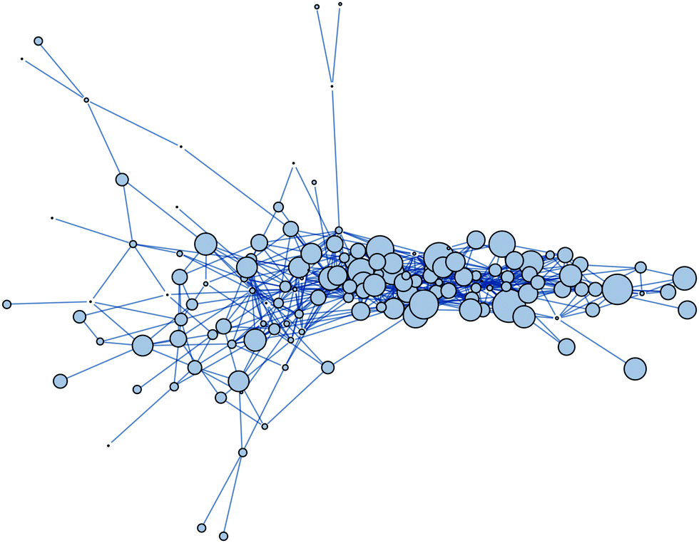 | ||
| Fig. 11 Network of minima for the NN model cost function [eqn (8)] applied to digit recognition. The size of the nodes is proportional to the number of neighbours. | ||
The benefits of analysing network properties of machine learning landscapes may be two-fold. One can attempt to construct more efficient and tailor-made algorithms to find the global minimum of machine learning problems by exploiting these network properties, for example, by navigating the ‘shortest path’ to the global minimum. We also obtain a quantitative description of the distance between a typical minimum from the best fit solution.
In the future, we plan to study further properties of the networks of minima for a variety of artificial neural networks and test the small-world and scale-free properties. We hope that these results may be useful in constructing algorithms to find the global minimum of non-convex machine learning cost functions.
VII. The p-spin model and machine learning
Many machine learning problems are solved via some kind of optimisation that makes use of gradient based methods, such as the stochastic gradient descent. Such algorithms utilise the local geometry of the landscape, and eventually iterations stop progressing when the norm of the (stochastic) gradients approach zero. This leads to the following general question: for a real valued function, what values do the critical points have? The answer certainly depends on the structure of the function we have at hand. In this section, we will examine two classes of functions: the Hamiltonian of the p-spin spherical glass, and the loss function that arises in the optimisation of a simple deep learning problem. In this section, the deep learning problem is the same as the one introduced in Section V with a larger hidden layer and zero regularisation. The functions have very different structures, and at first sight they do not appear to resemble one another in any meaningful way. However, we find that the two systems may exhibit similar characteristics in terms of the values of their critical points, in spite of the apparent differences.A. Concentration of critical points of the p-spin model
The Hamiltonian of a mean-field spin glass is a homogeneous polynomial of a given degree, where the coefficients of the polynomial describe the nature and strength of the interaction between the spins. Since the polynomial is homogeneous, a common choice is to restrict the variables (spins) to the unit sphere. We investigate what can be said about the minimisation problem if we choose the coefficients of this polynomial at random and independently from the standard normal distribution.First, we define the notation for the rest of the section. We consider real valued polynomials, H(w), where w is the vector of variables of H; the degree of the polynomial H is p. We define the dimension of the polynomial by the length of the vector w, so if w = (w1,…,wN) then H is an N-dimensional polynomial. A degree p polynomial is homogeneous polynomial if it satisfies the following condition for any real t:
| H(tw) = H((tw1,…,twN)) = tpH(w) | (11) |
Having defined the notation, we now clarify the connection between polynomials and spin glasses. Suppose the vector, w = (w1,…,wN), describes the states of N Ising spins that are +1 or −1. Then ∑wi2 = N, so that the distance to the origin is  . The continuous analogue of this model is a hypercube embedded in a sphere of radius
  . Therefore, we can interpret the Hamiltonian of a spherical, p-body, spin glass by a homogeneous polynomial of degree p. This formulation for spin systems has been studied extensively in ref. 112–114. From here on, we will explicitly denote the dimension and the degree of the polynomial in a subscript.
The simplest case is when the degree is p = 1 and the polynomial (Hamiltonian) becomes
 | (12) |
![[Doublestruck R]](https://www.rsc.org/images/entities/char_e175.gif) N are constrained to the sphere i.e.
N are constrained to the sphere i.e.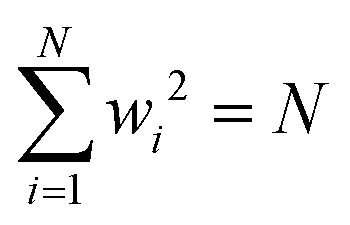 , where N is the number of spins. The coefficients xi ∼
 ![[scr N, script letter N]](https://www.rsc.org/images/entities/char_e52d.gif) (0,1) are independent and identically distributed standard normal random variables. For p = 1 there exist only two stationary points, one minimum and one maximum.
(0,1) are independent and identically distributed standard normal random variables. For p = 1 there exist only two stationary points, one minimum and one maximum.
When p = 2 the polynomial becomes
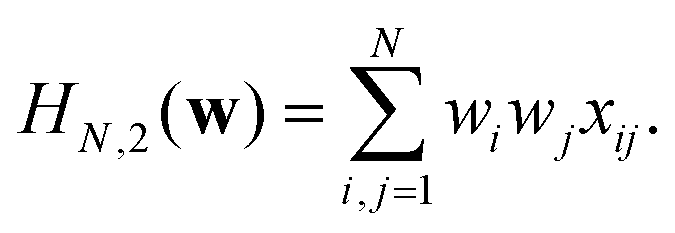 | (13) |
The picture is rather different when we look at polynomials with degree p > 2. When p = 3 the polynomial becomes
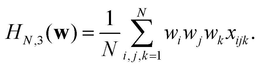 | (14) |
(0, 1), is chosen to make the extensive variables scale with N. In other words, when  , the variance of the Hamiltonian is proportional to N. With this convenient choice of normalization, the results of Auffinger et al.112 show that HN,3(w) has exponentially many stationary points, including exponentially many local minima (see ref. 117 for a complementary numerical study). In Fig. 12 we show the distribution of minima for the normalised HN,3(w) obtained by gradient descent for various system sizes, N, and for a single realisation of the coefficients. Since the variance of the Hamiltonian scales with N, dividing by N enables us to compare energies for systems with different dimensions. The initial point is chosen uniformly at random from the sphere. The step size is constant throughout the descent, until the norm of the gradient becomes smaller than 10−6. For small N the energies of the minima are broadly scattered. However as the number of spins increases, the distribution concentrates around a threshold. Further details of the calculations can be found in Sagun et al.99 (and ref. 118 for a complementary study).
 | ||
| Fig. 12 Histogram for the energies of points found by gradient descent with the Hamiltonian defined in eqn (14), comparing low-dimensional and high-dimensional systems. −E0 denotes the ground state, and −E∞ denotes the large N limit of the level for the bulk of the local minima. | ||
To obtain a more precise picture for the energy levels of critical points, we will focus on the level sets of the polynomial and count the number of critical points in the interior of a given level set. Here, the polynomial is assumed to be non-degenerate (its Hessian has nonzero eigenvalues). Then, a critical point is defined by a point whose gradient is the zero vector, and a critical point of index k has exactly k negative Hessian eigenvalues. Finally, our description of the number of critical points will be in the exponential form and in the asymptotic, large N, limit.
Following Auffinger et al., let 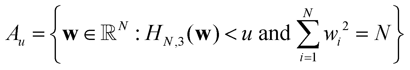 be the set of points in the domain of the function whose values lie below u. Also, let Ck(Au) denote the number of stationary (critical) points with index k in the set Au. Hence Ck(Au) counts the number of critical points with values below u. Then, the main theorem of ref. 112 produces the asymptotic expectation value
 ![[Doublestruck E]](https://www.rsc.org/images/entities/char_e168.gif) for the number of stationary points below energy u:
for the number of stationary points below energy u:
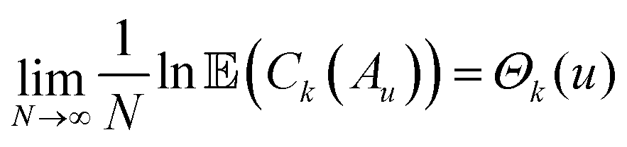 | (15) |
 and is bounded from below by −E0 ≈ −1.657. We therefore have a lower bound for the value of the ground state, and all stationary points exist in the energy band −E0 ≤ u ≤ −E∞.
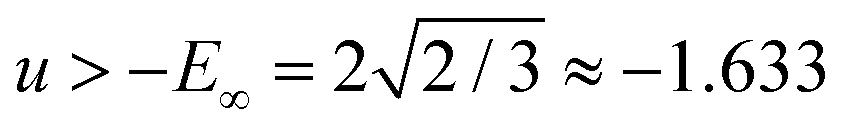
An inspection of the complexity function provides insight about the geometry at the bottom of the energy landscape (Fig. 13). The ground state is roughly at u = −1.657. For u ≥ −E∞ we do not see any local minima, because they all have values that are within the band −E0 ≤ u ≤ −E∞. Moreover, in the same band the stationary points of index k > 0 are outnumbered by local minima. In fact, this result holds hierarchically for all critical points of finite index (recall that the result is asymptotic so that by finite we mean fixing the index first and then taking the limit N → ∞). If we denote the x-axis intercept of the corresponding complexity function Θk as −Ek, with
| Θk(−Ek) = 0 for k = 1, 2,… | (16) |
 | ||
| Fig. 13 Plots of the complexity function Θk defined in eqn (15) for local minima, and saddles of index 1, 2 and 50. In the band (−E0, −E50) there are only critical points with indices {1, 2,…, 49}. | ||
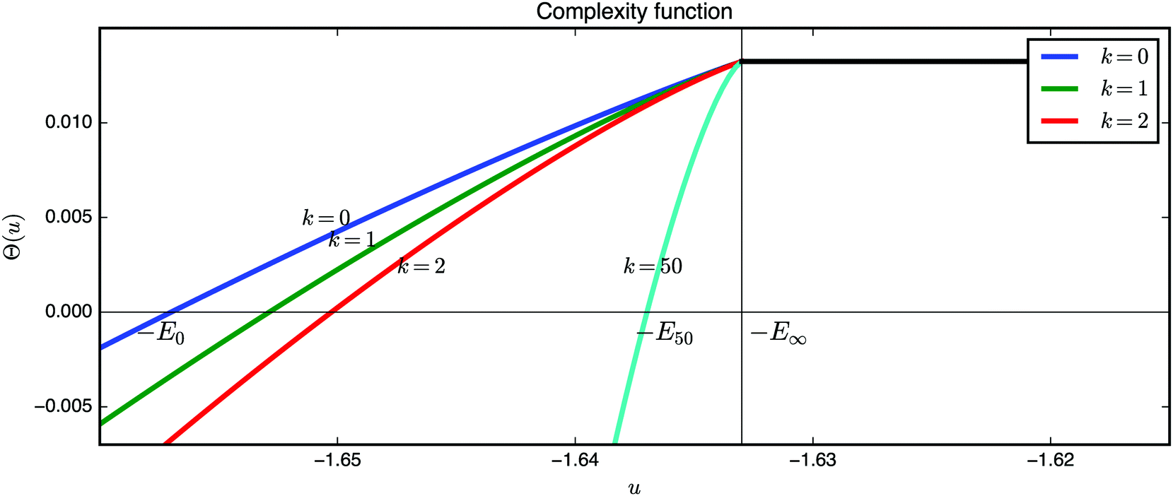
This scenario holds for the p-spin Hamiltonian with any p ≥ 3 where the threshold for the number of critical points is obtained asymptotically in the limit N → ∞. To demonstrate that it holds for reasonably small NFig. 14 shows the results for the p = 3 case with increasing dimensions. The concentration of local minima near the threshold increases rather quickly.
 | ||
| Fig. 14 Empirical variance of energies found by the gradient descent vs. the number of spins of the Hamiltonian defined in eqn (14). | ||
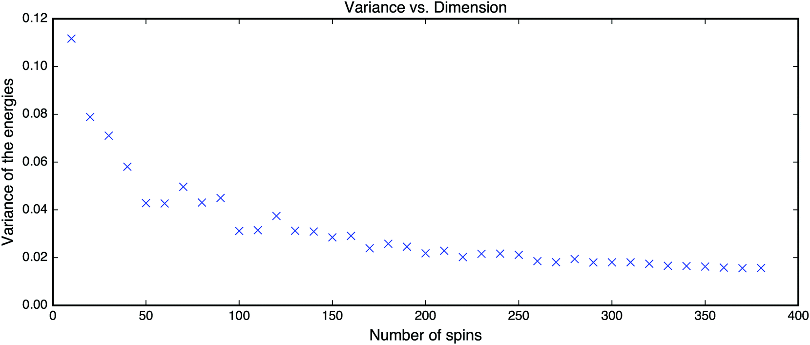
In Fig. 15 we show disconnectivity graphs for p = 3 spin spherical glass models with sizes N ∈ [50, 100] and fixed coefficients xijk ∼ (0,1). The landscape appears to become more frustrated already for small N, and the range over which local minima are found narrows with increasing system size, in agreement with the concentration phenomenon described in ref. 112.
 | ||
| Fig. 15 Disconnectivity graphs for p = 3 spin spherical glass models of size N ∈ [50, 100]. Each disconnectivity graph refers to a single realisation of the coefficients xijk ∼ (0,1). Frustration in the landscape is already visible for small system sizes, and the minima appear to concentrate over a narrowing band of energy values for as N increases. | ||
Interestingly, the concentration of stationary points phenomenon does not seem to be limited to the p-spin system. Related numerical results99 show that the same effect is observed for a slightly modified version of the random polynomial,  defined on the three-fold product of unit spheres. We do not yet have an analogue of the above theorem for Ĥ, so guidance from numerical results is particularly useful.
B. Machine learning landscapes and concentration of stationary points
The concept of complexity for a given function, as defined by the number and the nature of critical points on a given subset of the domain, gives rise to a description of the landscape as outlined above. If the energy landscape of machine learning problems is complex in this specific sense, we expect to see similar concentration phenomena in the optimisation of the corresponding loss functions. In fact, it is not straightforward to construct an analogue of the θ function as in eqn (15). However, we can empirically check whether optimisation stalls at a level above the ground state, as for the homogeneous polynomials with random coefficients described above.Let D := (x1,y1),…,(xn,yn) be n data points with input xi ∈ N, and label y ∈ ; and let G(w,x) = ŷ describe the output that approximates the label y parametrized by w ∈ M. Further, let (G(w,x),y) = (ŷ,y) be a non-negative loss function. Once we fix the dataset, we can focus on the averaged loss described by
 | (17) |
 | ||
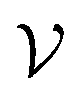
| Fig. 16 Training on linear, fully-connected MNIST networks (student networks) of various sizes. The labels for the network sizes are relative to the first network that is used to create new labels. For the larger and equally sized networks the ground state is known to lie at zero, yet the training stalls at a value around 0.016. | ||
We emphasise that the similarity between the p-spin Hamiltonian and the machine learning loss function lies only in the concentration phenomena, perhaps because the two functions share some underlying structure. It is likely that this observation of concentration in the two systems, spin glasses and deep learning, are due to different reasons that are peculiar to their organisation. It is also possible that such concentration behaviour is universal, in the sense that it can be observed in various non-convex and high dimensional systems for which the two systems above are just examples. However, if we wish to describe the ML landscape in terms of glassy behaviour, we might seek justification through the non-linearities in neural networks (the hidden layer in Fig. 1). In some sense, the non-linearity of a neural network is the key that introduces competing forces in which neurons can be inhibitory or exhibitory. This behaviour may introduce a similar structure to the signs of interaction coefficients in spins, introducing frustration. We note that these interpretations are rather speculative at present. Another problem that requires further research is identification of all critical points, not only the ones with low index. A more systematic way to identify the notion of complexity is through finding all of the critical points of a given function. A further challenge lies in the degeneracy of the systems in deep learning. The random polynomials that we considered have non-degenerate Hessian eigenvalue spectra for stationary points at the bottom of the landscape. However, a typical neural network has most Hessian eigenvalues near zero.119
Recently, a complementary study of the minima and saddle points of the p-spin model has been initiated using the numerical polynomial homotopy continuation method,120,121 which guarantees to find all the minima, transition states and higher index saddles for moderate sized systems.116,117 An advantage of this approach is that one can also analyse the variances of the number of minima, transition states, etc., providing further insight into the landscape of the p-spin model. A study for larger values of p, analysing the interpretation in terms of a deep learning network, is in progress.118
VIII. Basin volume calculations: quantifying the energy landscape
The enumeration of stationary points in the energy landscape provides a direct measure of complexity. This quantity is directly related to the landscape entropy89–92 (to be distinguished from the well entropy associated with the vibrational modes of each local minimum122) and is crucial for understanding the emergent dynamics and thermodynamics. In this context other important questions include determining the level of the stationary points (as we discussed in Section VII) and the volume of their basins of attraction. These volumes are of great practical interest because they provide an a priori measure of the probability of finding a particular minimum following energy minimisation. This probability is particularly important within the context of non-convex optimisation problems and machine learning, where an established protocol to quantify the landscape and the a priori outcome of learning is lacking.The development of general methods for enumerating the number of accessible microstates in a system, and ideally their individual probabilities, is therefore of great general interest. As discussed in Section VII, for a few specific cases there exist methods – either analytical or numerical – capable of producing exact estimates of these numbers. However, these techniques are either not sufficiently general or simply not practical for problems of interest. To date, at least two general and practical computational approaches have been developed. ‘Basin-sampling’55 employs a model anharmonic density of states for local minima organised in bins of potential energy, and has been applied to atomic clusters, including benchmark systems with double funnel landscapes that pose challenging issues for sampling. The mean basin volume (MBV) method developed by Frenkel and co-workers57,123–125 is similar in spirit to basin-sampling, but is based on thermodynamic integration and, being completely general, requires no assumptions on the shape of the basins (although thus far all examples are limited to the enumeration of the minima). MBV has been applied in the context of soft sphere packings and has facilitated the direct computation of the entropy in two123,124 and three57 dimensions. Furthermore, the technique has allowed for a direct test of the Edwards conjecture in two dimensions,126 suggesting that only at unjamming – when the system changes from a fluid to a solid, which is the density of practical significance for many granular systems – the entropy is maximal and all packings are equally probable.
Despite the high computational cost, the MBV underlying principle is straightforward. Assuming that the total configuration volume  of the energy landscape is known (simply
  = VN for an ideal gas of non-interacting atoms), if we can estimate the mean basin volume of all states, the number of minima is simply
 | (18) |
 , they will be sampled in proportion to the volume of the basin of attraction, and therefore the observed distribution of vbasin is biased. A detailed discussion of the unbiasing procedure for jammed soft-sphere packings is given in ref. 57. The Boltzmann-like entropy of the system is then simply SB = lnΩ − lnN!. Similarly, from knowledge of the biased (observed) distribution of basin volumes vi alone, one can compute the Gibbs-like (or Shannon) entropy
  , where
  is the relative probability for minimum i.
The computation of the basin volume is performed by thermodynamic integration. In essence, we perform a series of Markov chain Monte Carlo random walks within the basin applying different biases to the walkers and, from the distributions of displacements from a reference point (usually the minimum), compute the dimensionless free energy difference between a region of known volume and that of an unbiased walker. In other words
fbasin = fref + (![[f with combining circumflex]](https://www.rsc.org/images/entities/i_char_0066_0302.gif) basin − ref) basin − ref) | (19) |
v and the hat refers to quantities estimated up to an additive constant by the free energy estimator of choice, either Frenkel–Ladd57,127 or the multi-state Bennet acceptance ratio method (MBAR).125,128 The high computational cost of these calculations is due to the fact that, in order to perform a random walk in the body of the basin, a full energy minimisation is required to check whether the walker has overstepped the basin boundary.
Recently the approach has been validated when the dynamics determining the basin of attraction are stochastic in nature,129 which is precisely the situation encountered in the training by stochastic optimisation of neural networks and other non-convex machine learning problems. The extension of these techniques to machine learning is another exciting prospect, as it would provide a general protocol for quantifying the machine learning landscape and establishing, for instance, whether the different solutions to learning occur with different probabilities and, if so, what their distribution is. This characterisation of the learning problem could help to develop better models, as well as better training algorithms.
IX. Conclusions
In this Perspective we have applied theory and computational techniques from the potential energy landscapes field2 to analyse problems in machine learning. The multiple solutions that can result from optimising fitting functions to training data define a machine learning landscape,23 where the cost function that is minimised in training takes the place of the molecular potential energy function. This machine learning landscape can be explored and visualised using methodology transferred directly from the potential energy landscape framework. We have illustrated how this approach can be used through examples taken from recent work, including analogies with thermodynamic properties, such as the heat capacity, which reports on the structure of the equilibrium properties of the solution space as a function of a fictitious temperature parameter. The interpretation of ML landscapes in terms of analogues of molecular structure and transition rates is an intriguing target for future work.Energy landscape methods may provide a novel way of addressing one of the most intriguing questions in the machine learning research, namely why does machine learning work so well? One way to ask this question more quantitatively is to investigate why we can usually find a good candidate for the global minimum of a machine learning cost function relatively quickly, even in the presence of so many local minima. The present results suggest that the landscape for a range of models are single-funnel-like, i.e. the largest basin of attraction is that of the global minimum, and the downhill barriers that separate it from local minima are relatively small. This organisation facilitates rapid relaxation to the global minimum for global optimisation techniques, such as basin-hopping. Another possible explanation is that many local minima provide fits that are competitive with the global minimum.96,97,99 In fact, these two scenarios are compatible, so that global optimisation leads us downhill on the landscape, where we encounter local minima that provide predictions or classifications of useful accuracy.
The ambition to develop more fundamental connections between machine learning disciplines and computational chemical physics could be very productive. For example, there have recently been many physics-inspired contributions in machine learning, including thermodynamics-based models for rational decision-making,130 generative models from non-equilibrium simulations.131 The hope is that such connections can provide better intuition about the machine learning problems in question, and perhaps also the underlying physical theories used to understand them.
Acknowledgements
It is a pleasure to acknowledge discussions with Prof. Daan Frenkel, Dr Victor Ruehle, Dr Peter Wirnsberger, Prof. Gérard Ben Arous, and Prof. Yann Lecun. This research was funded by EPSRC grant EP/I001352/1, the Gates Cambridge Trust, and the ERC. DM was in the Department of Applied and Computational Mathematics and Statistics when this work was performed, and his current affiliation is Department of Systems, United Technologies Research Center, East Hartford, CT, USA.References
- S. T. Chill, J. Stevenson, V. Ruehle, C. Shang, P. Xiao, J. D. Farrell, D. J. Wales and G. Henkelman, J. Chem. Theory Comput., 2014, 10, 5476 CrossRef CAS PubMed.
- D. J. Wales, Energy Landscapes, Cambridge University Press, Cambridge, 2003 Search PubMed.
- D. J. Wales, Curr. Opin. Struct. Biol., 2010, 20, 3 CrossRef CAS PubMed.
- D. J. Wales, M. A. Miller and T. R. Walsh, Nature, 1998, 394, 758 CrossRef CAS.
- D. J. Wales, Philos. Trans. R. Soc., A, 2005, 363, 357 CrossRef CAS PubMed.
- V. K. de Souza and D. J. Wales, J. Chem. Phys., 2008, 129, 164507 CrossRef PubMed.
- J. D. Bryngelson, J. N. Onuchic, N. D. Socci and P. G. Wolynes, Proteins, 1995, 21, 167 CrossRef CAS PubMed.
- J. N. Onuchic, Z. Luthey-Schulten and P. G. Wolynes, Annu. Rev. Phys. Chem., 1997, 48, 545 CrossRef CAS PubMed.
- D. Chakrabarti and D. J. Wales, Soft Matter, 2011, 7, 2325 RSC.
- Y. Chebaro, A. J. Ballard, D. Chakraborty and D. J. Wales, Sci. Rep., 2015, 5, 10386 CrossRef PubMed.
- P. G. Mezey, Potential Energy Hypersurfaces, Elsevier, Amsterdam, 1987 Search PubMed.
- F. Noé and S. Fischer, Curr. Opin. Struct. Biol., 2008, 18, 154 CrossRef PubMed.
- D. Prada-Gracia, J. Gómez-Gardenes, P. Echenique and F. Fernando, PLoS Comput. Biol., 2009, 5, e1000415 Search PubMed.
- D. J. Wales, Mol. Phys., 2002, 100, 3285 CrossRef CAS.
- C. Dellago, P. G. Bolhuis and D. Chandler, J. Chem. Phys., 1998, 108, 9236 CrossRef CAS.
- D. Passerone and M. Parrinello, Phys. Rev. Lett., 2001, 87, 108302 CrossRef CAS PubMed.
- W. E, W. Ren and E. Vanden-Eijnden, Phys. Rev. B: Condens. Matter Mater. Phys., 2002, 66, 052301 CrossRef.
- O. M. Becker and M. Karplus, J. Chem. Phys., 1997, 106, 1495 CrossRef CAS.
- J. P. K. Doye, M. A. Miller and D. J. Wales, J. Chem. Phys., 1999, 110, 6896 CrossRef CAS.
- J. N. Murrell and K. J. Laidler, Trans. Faraday Soc., 1968, 64, 371 RSC.
- R. Collobert, F. Sinz, J. Weston and L. Bottou, Proceedings of the 23rd International Conference on Machine Learning, ICML '06, ACM, New York, NY, USA, 2006, pp. 201–208.
- M. Pavlovskaia, K. Tu and S.-C. Zhu, Mapping the Energy Landscape of Non-convex Optimization Problems, in Energy Minimization Methods in Computer Vision and Pattern Recognition, ed. X.-C. Tai, E. Bae, T. F. Chan and M. Lysaker, 10th International Conference, EMMCVPR 2015, Springer International Publishing, Hong Kong, China, 2015, pp. 421–435 Search PubMed.
- A. J. Ballard, J. D. Stevenson, R. Das and D. J. Wales, J. Chem. Phys., 2016, 144, 124119 CrossRef PubMed.
- R. Das and D. J. Wales, Phys. Rev. E, 2016, 93, 063310 CrossRef PubMed.
- S. Manzhos and T. Carrington, J. Chem. Phys., 2006, 125, 084109 CrossRef PubMed.
- S. Houlding, S. Y. Liem and P. L. A. Popelier, Int. J. Quantum Chem., 2007, 107, 2817 CrossRef CAS.
- J. Behler, R. Martoňák, D. Donadio and M. Parrinello, Phys. Rev. Lett., 2008, 100, 185501 CrossRef PubMed.
- C. M. Handley, G. I. Hawe, D. B. Kell and P. L. A. Popelier, Phys. Chem. Chem. Phys., 2009, 11, 6365 RSC.
- J. Behler, S. Lorenz and K. Reuter, J. Chem. Phys., 2007, 127, 014705 CrossRef PubMed.
- J. Li and H. Guo, J. Chem. Phys., 2015, 143, 214304 CrossRef PubMed.
- K. Shao, J. Chen, Z. Zhao and D. H. Zhang, J. Chem. Phys., 2016, 145, 071101 CrossRef PubMed.
- C. M. Handley and P. L. A. Popelier, J. Phys. Chem. A, 2010, 114, 3371 CrossRef CAS PubMed.
- T. B. Blank, S. D. Brown, A. W. Calhoun and D. J. Doren, J. Chem. Phys., 1995, 103, 4129 CrossRef CAS.
- D. F. R. Brown, M. N. Gibbs and D. C. Clary, J. Chem. Phys., 1996, 105, 7597 CrossRef CAS.
- H. Gassner, M. Probst, A. Lauenstein and K. Hermansson, J. Phys. Chem. A, 1998, 102, 4596 CrossRef CAS.
- P. J. Ballester and J. B. O. Mitchell, Bioinformatics, 2010, 26, 1169 CrossRef CAS PubMed.
- A. W. Long and A. L. Ferguson, J. Phys. Chem. B, 2014, 118, 4228 CrossRef CAS PubMed.
- B. A. Lindquist, R. B. Jadrich and T. M. Truskett, J. Chem. Phys., 2016, 145, 111101 CrossRef.
- Z. D. Pozun, K. Hansen, D. Sheppard, M. Rupp, K. R. Muller and G. Henkelman, J. Chem. Phys., 2012, 136, 174101 CrossRef PubMed.
- C. Cortes and V. Vapnik, Mach. Learn., 1995, 20, 273 Search PubMed.
- Z. Li and H. A. Scheraga, Proc. Natl. Acad. Sci. U. S. A., 1987, 84, 6611 CrossRef CAS.
- Z. Li and H. A. Scheraga, J. Mol. Struct., 1988, 179, 333 CrossRef.
- D. J. Wales and J. P. K. Doye, J. Phys. Chem. A, 1997, 101, 5111 CrossRef CAS.
- J. Nocedal, Math. Comput., 1980, 35, 773 CrossRef.
- S. A. Trygubenko and D. J. Wales, J. Chem. Phys., 2004, 120, 2082 CrossRef CAS PubMed.
- S. A. Trygubenko and D. J. Wales, J. Chem. Phys., 2004, 121, 6689 CrossRef CAS PubMed.
- G. Henkelman, B. P. Uberuaga and H. Jónsson, J. Chem. Phys., 2000, 113, 9901 CrossRef CAS.
- G. Henkelman and H. Jónsson, J. Chem. Phys., 2000, 113, 9978 CrossRef CAS.
- L. J. Munro and D. J. Wales, Phys. Rev. B: Condens. Matter Mater. Phys., 1999, 59, 3969 CrossRef CAS.
- Y. Zeng, P. Xiao and G. Henkelman, J. Chem. Phys., 2014, 140, 044115 CrossRef PubMed.
- Pele: Python energy landscape explorer, http://https://github.com/pele-python/pele.
- D. J. Wales, GMIN: a program for basin-hopping global optimisation, basin-sampling, and parallel tempering, http://www-wales.ch.cam.ac.uk/software.html Search PubMed.
- D. J. Wales, OPTIM: a program for geometry optimisation and pathway calculations, http://www-wales.ch.cam.ac.uk/software.html Search PubMed.
- D. J. Wales, PATHSAMPLE: a program for generating connected stationary point databases and extracting global kinetics, http://www-wales.ch.cam.ac.uk/software.html Search PubMed.
- D. J. Wales, Chem. Phys. Lett., 2013, 584, 1 CrossRef CAS.
- F. Noé, D. Krachtus, J. C. Smith and S. Fischer, J. Chem. Theory Comput., 2006, 2, 840 CrossRef PubMed.
- S. Martiniani, K. J. Schrenk, J. D. Stevenson, D. J. Wales and D. Frenkel, Phys. Rev. E, 2016, 93, 012906 CrossRef PubMed.
- K. Swersky, J. Snoek and R. P. Adams, 2014, arXiv:1406.3896 [stat.ML].
- D. J. Wales, J. Chem. Soc., Faraday Trans., 1992, 88, 653 RSC.
- D. J. Wales, J. Chem. Soc., Faraday Trans., 1993, 89, 1305 RSC.
- D. Asenjo, J. D. Stevenson, D. J. Wales and D. Frenkel, J. Phys. Chem. B, 2013, 117, 12717 CrossRef CAS PubMed.
- J. E. Jones and A. E. Ingham, Proc. R. Soc. A, 1925, 107, 636 CrossRef CAS.
- P. M. Axilrod and E. Teller, J. Chem. Phys., 1943, 11, 299 CrossRef.
- C. G. Broyden, J. Inst. Math. Its Appl., 1970, 6, 76 CrossRef.
- R. Fletcher, Comput. J., 1970, 13, 317 CrossRef.
- D. Goldfarb, Math. Comput., 1970, 24, 23 CrossRef.
- D. F. Shanno, Math. Comput., 1970, 24, 647 CrossRef.
- C. M. Bishop, Pattern Recognition and Machine Learning, Springer, New York, 2006 Search PubMed.
- T. Hastie, R. Tibshirani and J. Friedman, The Elements of Statistical Learning, Springer, New York, 2009 Search PubMed.
- M. Page and J. W. McIver, J. Chem. Phys., 1988, 88, 922 CrossRef CAS.
- J. P. K. Doye, Phys. Rev. E, 2000, 62, 8753 CrossRef CAS.
- F. H. Stillinger and T. A. Weber, J. Stat. Phys., 1988, 52, 1429 CrossRef.
- F. H. Stillinger and T. A. Weber, Science, 1984, 225, 983 CAS.
- D. J. Wales and J. P. K. Doye, J. Chem. Phys., 2003, 119, 12409 CrossRef CAS.
- D. J. Wales and J. P. K. Doye, J. Chem. Phys., 1995, 103, 3061 CrossRef CAS.
- D. J. Wales, Mol. Phys., 1993, 78, 151 CrossRef CAS.
- F. H. Stillinger, Science, 1995, 267, 1935 CAS.
- B. Strodel and D. J. Wales, Chem. Phys. Lett., 2008, 466, 105 CrossRef CAS.
- V. A. Sharapov, D. Meluzzi and V. A. Mandelshtam, Phys. Rev. Lett., 2007, 98, 105701 CrossRef PubMed.
- M. T. Oakley, R. L. Johnston and D. J. Wales, Phys. Chem. Chem. Phys., 2013, 15, 3965 RSC.
- J. P. Neirotti, F. Calvo, D. L. Freeman and J. D. Doll, J. Chem. Phys., 2000, 112, 10340 CrossRef CAS.
- F. Calvo, J. P. Neirotti, D. L. Freeman and J. D. Doll, J. Chem. Phys., 2000, 112, 10350 CrossRef CAS.
- V. A. Mandelshtam, P. A. Frantsuzov and F. Calvo, J. Phys. Chem. A, 2006, 110, 5326 CrossRef CAS PubMed.
- V. A. Sharapov and V. A. Mandelshtam, J. Phys. Chem. A, 2007, 111, 10284 CrossRef CAS PubMed.
- F. Calvo, Phys. Rev. E: Stat., Nonlinear, Soft Matter Phys., 2010, 82, 046703 CrossRef CAS PubMed.
- R. M. Sehgal, D. Maroudas and D. M. Ford, J. Chem. Phys., 2014, 140, 104312 CrossRef PubMed.
- D. J. Wales, Mol. Phys., 2004, 102, 891 CrossRef CAS.
- M. Picciani, M. Athenes, J. Kurchan and J. Tailleur, J. Chem. Phys., 2011, 135, 034108 CrossRef PubMed.
- F. Sciortino, W. Kob and P. Tartaglia, J. Phys.: Condens. Matter, 2000, 12, 6525 CrossRef CAS.
- T. V. Bogdan, D. J. Wales and F. Calvo, J. Chem. Phys., 2006, 124, 044102 CrossRef PubMed.
- G. Meng, N. Arkus, M. P. Brenner and V. N. Manoharan, Science, 2010, 327, 560 CrossRef CAS PubMed.
- D. J. Wales, ChemPhysChem, 2010, 11, 2491 CrossRef CAS PubMed.
- R. Das and D. J. Wales, Chem. Phys. Lett., 2017, 667, 158 CrossRef CAS.
- Y. Lecun, L. Bottou, Y. Bengio and P. Haffner, Proc. IEEE, 1998, 86, 2278 CrossRef.
- See the MNIST database: http://yann.lecun.com/exdb/mnist.
- Y. Dauphin, R. Pascanu, Ç. Gülçehre, K. Cho, S. Ganguli and Y. Bengio, CoRR abs/1406.2572, 2014.
- A. J. Bray and D. S. Dean, Phys. Rev. Lett., 2007, 98, 150201 CrossRef PubMed.
- A. Choromanska, M. Henaff, M. Mathieu, G. Ben Arous and Y. LeCun, CoRR abs/1412.0233, 2014.
- L. Sagun, V. U. Güney, G. Ben Arous and Y. LeCun, ICLR2015 Workshop Contribution, 2014, arXiv:1412.6615.
- The misclassification distance can also be viewed as the Hamming distance between misclassification vectors of the two minima in question.
- J. P. K. Doye, Phys. Rev. Lett., 2002, 88, 238701 CrossRef PubMed.
- J. P. K. Doye and C. P. Massen, J. Chem. Phys., 2005, 122, 084105 CrossRef PubMed.
- D. Mehta, J. Chen, D. Z. Chen, H. Kusumaatmaja and D. J. Wales, Phys. Rev. Lett., 2016, 117, 028301 CrossRef PubMed.
- M. E. J. Newman, Networks: An Introduction, Oxford University Press, 2010 Search PubMed.
- S. H. Strogatz, Nature, 2001, 410, 268 CrossRef CAS PubMed.
- J. W. R. Morgan, D. Mehta and D. J. Wales, to appear.
- D. J. Watts and S. H. Strogatz, Nature, 1998, 393, 440 CrossRef CAS PubMed.
- D. J. Wales, J. P. K. Doye, M. A. Miller, P. N. Mortenson and T. R. Walsh, Adv. Chem. Phys., 2000, 115, 1 CrossRef.
- J. P. K. Doye, Phys. Rev. Lett., 2002, 88, 238701 CrossRef PubMed.
- J. M. Carr and D. J. Wales, J. Phys. Chem. B, 2008, 112, 8760 CrossRef CAS PubMed.
- A.-L. Barabási and R. Albert, Science, 1999, 286, 509 CrossRef.
- A. Auffinger, G. Ben Arous and J. Černý, Commun. Pure Appl. Math., 2013, 66, 165 CrossRef.
- A. Auffinger and G. B. Arous, et al. , Ann. Probab., 2013, 41, 4214 CrossRef.
- A. Auffinger and W.-K. Chen, 2017, arXiv:1702.08906, arXiv preprint.
- Y. V. Fyodorov and P. Le Doussal, J. Stat. Phys., 2014, 154, 466 CrossRef.
- D. Mehta, J. D. Hauenstein, M. Niemerg, N. J. Simm and D. A. Stariolo, Phys. Rev. E: Stat., Nonlinear, Soft Matter Phys., 2015, 91, 022133 CrossRef PubMed.
- D. Mehta, D. A. Stariolo and M. Kastner, Phys. Rev. E: Stat., Nonlinear, Soft Matter Phys., 2013, 87, 052143 CrossRef PubMed.
- D. Mehta, H. Sidky, Y. Dauphin and J. W. Whitmer, to appear.
- L. Sagun, L. Bottou and Y. LeCun, 2016, arXiv:1611.07476, arXiv preprint.
- A. J. Sommese and C. W. Wampler, The numerical solution of systems of polynomials arising in engineering and science, World Scientific, 2005, vol. 99 Search PubMed.
- D. Mehta, Phys. Rev. E: Stat., Nonlinear, Soft Matter Phys., 2011, 84, 025702 CrossRef PubMed.
- L. Berthier and D. Coslovich, Proc. Natl. Acad. Sci. U. S. A., 2014, 111, 11668 CrossRef CAS PubMed.
- N. Xu, D. Frenkel and A. J. Liu, Phys. Rev. Lett., 2011, 106, 245502 CrossRef PubMed.
- D. Asenjo, F. Paillusson and D. Frenkel, Phys. Rev. Lett., 2014, 112, 098002 CrossRef PubMed.
- S. Martiniani, K. J. Schrenk, J. D. Stevenson, D. J. Wales and D. Frenkel, Phys. Rev. E, 2016, 94, 031301 CrossRef PubMed.
- S. Martiniani, K. J. Schrenk, K. Ramola, B. Chakraborty and D. Frenkel, 2016, arXiv:1610.06328, arXiv preprint.
- D. Frenkel and A. J. C. Ladd, J. Chem. Phys., 1984, 81, 3188 CrossRef CAS.
- M. R. Shirts and J. D. Chodera, J. Chem. Phys., 2008, 129, 124105 CrossRef PubMed.
- D. Frenkel, K. J. Schrenk and S. Martiniani, 2016, arXiv:1612.06131, arXiv preprint.
- P. A. Ortega and D. A. Braun, Proc. R. Soc. London, Ser. A, 2013, 469 DOI:10.1098/rspa.2012.0683.
- J. Sohl-Dickstein, E. A. Weiss, N. Maheswaranathan and S. Ganguli, CoRR abs/1503.03585, 2015.
| This journal is © the Owner Societies 2017 |