
 Open Access Article
 This Open Access Article is licensed under a
 Creative Commons Attribution 3.0 Unported Licence
Determination of the diffusion coefficient of hydrogen ion in hydrogels†
Gábor
Schuszter‡
a,
Tünde
Gehér-Herczegh‡
a,
Árpád
Szűcs
a,
Ágota
Tóth
a and
Dezső
Horváth
 *b
*b
aDepartment of Physical Chemistry and Materials Science, Rerrich Béla ter 1., 6720 Szeged, Hungary
bDepartment of Applied and Environmental Chemistry, Rerrich Béla ter 1., 6720 Szeged, Hungary. E-mail: horvathd@chem.u-szeged.hu; Fax: +36 62/546-482; Tel: +36 62/544-614
First published on 11th April 2017
Abstract
The role of diffusion in chemical pattern formation has been widely studied due to the great diversity of patterns emerging in reaction–diffusion systems, particularly in H+-autocatalytic reactions where hydrogels are applied to avoid convection. A custom-made conductometric cell is designed to measure the effective diffusion coefficient of a pair of strong electrolytes containing sodium ions or hydrogen ions with a common anion. This together with the individual diffusion coefficient for sodium ions, obtained from PFGSE-NMR spectroscopy, allows the determination of the diffusion coefficient of hydrogen ions in hydrogels. Numerical calculations are also performed to study the behavior of a diffusion–migration model describing ionic diffusion in our system. The method we present for one particular case may be extended for various hydrogels and diffusing ions (such as hydroxide) which are relevant e.g. for the development of pH-regulated self-healing mechanisms and hydrogels used for drug delivery.
1 Introduction
Although diffusion is usually considered to be slow as a transport mechanism, it plays an important role in many applications, especially when the length scale of the problem is microscopic or the time scale is sufficiently long. In these cases, the difference in the diffusion properties of chemical species may significantly affect the output. This effect of varying diffusion may be represented via reaction–diffusion driven pattern formation, where visible patterns facilitate the understanding of the underlying interactions.Such chemical systems have been thoroughly investigated in the past few decades by both numerical studies and experimental studies. Notably in the early 1990s, stationary Turing patterns1 were first observed and since then well-designed experimental methods2,3 have been developed to produce these phenomena in various systems. Numerical simulations have shown that a rich variety of complex spatiotemporal patterns can be created using simple models with autocatalytic chemical reactions influenced by diffusion.4 The resulting patterns may be e.g. spirals, stripes, hexagons, lamellae, and self-replicating spots which have also been reproduced experimentally in acid auto-activated reactions in hydrogel media.5 Such intriguing acid auto-activated systems including, among others, the thiourea–iodate–sulfite reaction which exhibited Turing bifurcation, the clock reaction bromate–sulfite system,6 the mixed Landolt-type pH-oscillator bromate–sulfite–ferrocyanide reaction,7 and other halogen-free hydrogen–peroxide driven reactions8 are all examples where phenomena like stationary patterns, spatial bistability, travelling acid–base fronts or spatiotemporal oscillations have been observed. Propagating fronts have been studied in e.g. the iodate–arsenous acid9 or the chlorite–tetrathionate reactions as well.10,11 In other systems, the diffusion of hydroxide ions plays an important role regarding the macroscopic patterns.12 A common feature of these systems is that the pattern formation is essentially controlled by the diffusion rate of the chemical species present in the system, particularly regarding the autocatalyst that is often the hydrogen ion. Its fast hopping mechanism in water results in a high diffusion coefficient value and a long-range activation process that can significantly influence the nonlinear behavior of the system – e.g. oscillatory states – as shown by numerical studies.13
Hydrogels such as agarose, gelatin or polyacrylamide are fundamentally used as reaction media for chemical pattern formation for the purpose of eliminating macroscopic convection. In addition, pH-sensitive hydrogels are also applied to make artificial molecular motors which are able to contract and collapse depending on the actual pH of the medium.14,15 In the electrolyte diodes developed for analytical purposes, hydrogels are commonly utilized as connecting elements between the acidic and alkaline reservoirs.16,17 Environmental-sensitive hydrogels are frequently used materials not only in chemistry and physics but also in biomedical applications, such as tissue engineering and drug delivery.18,19 For those kinds of applications, the improvement of shear-thinning and self-healing properties together with a reduced response time is essential and may be tuned by changes in pH or temperature.20–22 The case of pH change links again the diffusion properties of hydrogen ions in the actual gel.
For each of those purposes, the quality and concentration of the gel alongside with additional substances can remarkably affect the diffusion of chemical species. Regarding pattern formation, the modified diffusion can be tracked via different pattern morphologies in other types of reaction–diffusion systems such as Liesegang patterns.23,24 Empirical evidence implies that the diffusion rate of chemical species – in particular that of H+ – may reasonably change in hydrogels compared to dilute aqueous solutions due to structural or chemical interactions; however, the extent of this change cannot be trivially inferred. So far in numerical studies attempting to model pattern formation in acid auto-activated systems, only theoretical values and approximations have been available for the diffusion coefficients of the relevant species in hydrogels. Therefore our aim is to provide practical values for ionic diffusion coefficients, particularly DH+ under frequent experimental conditions.
Special attention has to be given to finding the most appropriate experimental technique due to the challenging circumstances. Several well-established and accessible techniques may be mentioned for determining diffusion coefficients e.g. using radioactive tracers,25 fluorescence methods,26,27 holographic laser interferometry,28 the refractive index method,29 nuclear magnetic resonance techniques,30etc. Evidently, radioactive and fluorescence methods are not suitable for following the movement of hydrogen ions; furthermore, in occasionally opalescent hydrogels, such as agarose or agar–agar, the efficiency of interferometric and refractive methods may be significantly reduced in the case of small ions, even though these techniques have been reliably used for studying larger species such as protein macromolecules. Pulsed-field gradient spin echo (PFGSE) NMR spectroscopy can be readily applied to measure a large number of small individual ions including 1H nucleus;31,32 however, hydrogel media generate excessive water signals that cannot be suppressed without eliminating the relevant signal of free protons as well.
The scientific problem, namely to determine relevant individual diffusion coefficients of ions experimentally if the surroundings also contain the same ion in the immobilized form, is not solved yet. Therefore, as we present the particular case of the hydrogen ion in agarose gel, we have developed a complex experimental procedure as a combination of available and effective techniques. This paper introduces our methods and demonstrates the experimental results accompanied by numerical modeling of ionic diffusion.
For an easier understanding we present the rather complex results in separate parts regarding either the relevant experimental techniques or the performed modeling. First we introduce the theoretical background of the method including the basis of conductance measurements and of PFGSE-NMR. We then describe the actual conductometric cell followed by its electric properties and the diffusion–migration model. We come to the experimental section which contains two major parts:
(1) Conductance measurements to obtain relevant effective diffusion coefficients for electrolytes;
(2) PFGSE-NMR measurements to obtain individual diffusion coefficients.
In the end, we combine all those data in Section 6 to present our final results considering the diffusion coefficient of the hydrogen ion in agarose gel.
2 Theoretical background
Among many other techniques, a conductance method was developed by Harned and French for the purpose of determining the effective diffusion coefficient (Deff) of electrolytes in dilute aqueous solutions.33–38 They aimed for maximum simplicity concerning the mathematical treatment of the experimental data. Here we recall some of their results and formulation for easier understanding.The diffusional cell in the shape of a cuvette with length a contained two pairs of platinum electrodes placed at a distance ξ from both ends (see Fig. 1). The medium confined by the cuvette can be considered one dimensional, for which Fick's second law
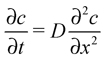 | (1) |
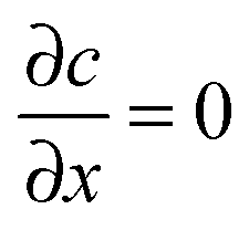 at x = 0 and x = a has a solution in the form of a Fourier cosine series as
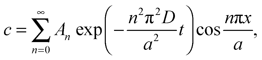 | (2) |
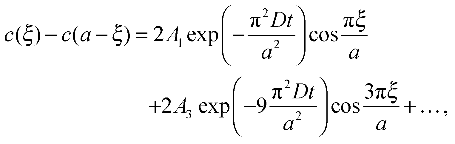 | (3) |
 cell geometry eliminating the term with n = 3. The right-hand side is then reduced to a more simplified form, given that after sufficient time – due to the rapid convergence of the higher order exponentials – only the first term will have significant contribution, leading to
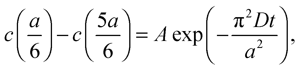 | (4) |
 .
.
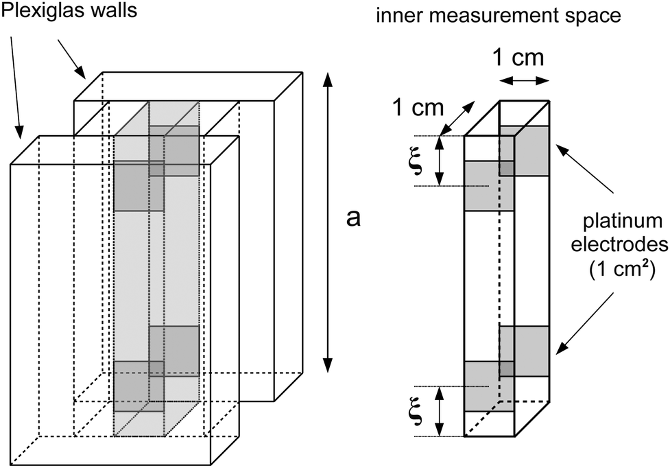 | ||
| Fig. 1 Design of the conductometric cell: the height of the inner space is a = 6 cm, the center of each square shaped platinum electrode embedded in the Plexiglas walls is placed ξ = 1 cm far from the top or bottom of the cell. The inner space is filled with a 6 cm3 total volume of the hydrogel. | ||
In dilute solutions, the difference 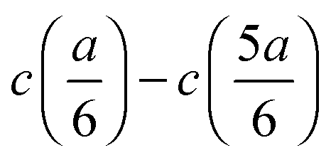 can be considered to be proportional to the difference in specific conductivity κ at the same positions, i.e., CtopGtop–CbottomGbottom, where Ctop and Cbottom are the cell constants regarding the upper and the lower pairs of electrodes, while G is the measured conductance. When this difference in G is substituted into eqn (4), a direct formula
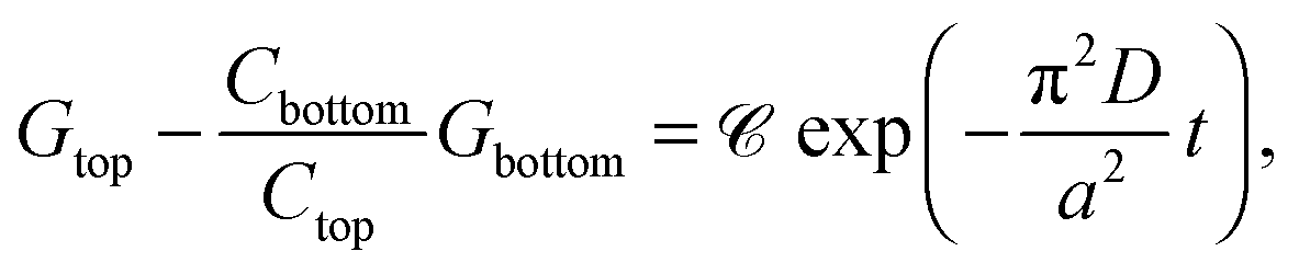 | (5) |
![[capital script C]](https://www.rsc.org/images/entities/char_e522.gif) stands for the preexponential coefficient, is obtained that allows the determination of diffusion coefficients directly from conductance values. Linearization
stands for the preexponential coefficient, is obtained that allows the determination of diffusion coefficients directly from conductance values. Linearization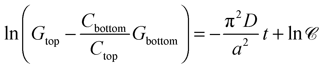 | (6) |
The other essential equation relies in the fact that the diffusion coefficients of individual ions cannot be determined directly using this method, since all ionic components in the system contribute to conductance. However, a simple formula exists for the effective diffusion coefficient (Deff) for 1![[thin space (1/6-em)]](https://www.rsc.org/images/entities/char_2009.gif) :1 binary strong electrolytes
:1 binary strong electrolytes
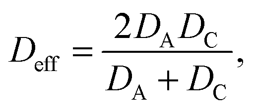 | (7) |
One experimental technique capable of measuring individual ionic diffusion coefficients is based on PFGSE-NMR spectroscopy.31,32 In the presence of a magnetic field gradient g, an exponentially decaying signal I(g) can be detected according to the Stejskal–Tanner equation:
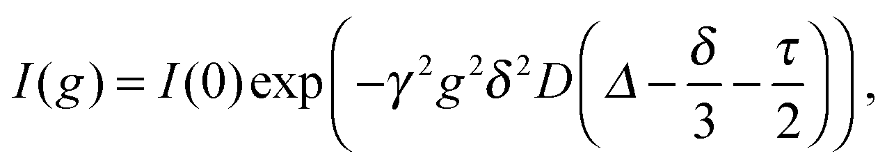 | (8) |
Although PFGSE-NMR spectroscopy cannot be directly used for measuring the diffusion coefficient of H+ due to the excessive water signal in hydrogels, it is available for other small ions with NMR-active nuclei. Therefore, the isotope 23Na is chosen to obtain an individual DC value in eqn (7) for sodium ions, while conductance measurements are performed for NaCl and HCl solutions – electrolytes with a common anion – under the same conditions. To combine all results, eqn (7) is applied twice, first to calculate DCl− from DNa+ (via NMR) and Deff,NaCl (via conductance), then a second time using DCl− (from the previous step) and Deff,HCl (via conductance) to determine the final diffusion coefficient of hydrogen ions.
To verify the selection of the 23Na nucleus, the authors note that hydrogen chloride solution may be chosen for conductance measurements as a suitable electrolyte that contains H+ as the cation; however, the properties of NMR active chlorine isotopes such as their relaxation times make chloride ions unfavorable for PFGSE-NMR measurements.
3 Cell design
For determining the required effective diffusion coefficients of sodium chloride and hydrogen chloride in a hydrogel, we have designed a conductometric cell based on the original concept of Harned and French.33 The height of the cell a = 6 cm while its cross section is 1 cm × 1 cm. This inner measurement space enclosed by Plexiglas walls was constructed with an open top and bottom face that could be filled with the hydrogel and then sealed airtight, as illustrated in Fig. 1.To measure the change of conductance while an adjusted concentration gradient of the main diffusing electrolyte diminishes with time, four pieces of square shaped 1 cm2 platinum foils were embedded in the Plexiglas walls opposite to each other thus forming two pairs of electrodes. The center of each electrode was located ξ = 1 cm from both the top and bottom ends. These a and ξ values hence correspond to the 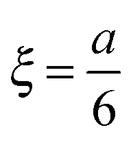 ratio requirement introduced by Harned and French and therefore allow us to use eqn (5) for the evaluation in our experiments. For consistent measurements, the cell was always positioned in the same orientation and the ends were marked permanently in order for the electrode pairs to become distinguishable as the top pair and the bottom pair (as referred to henceforth). Each embedded platinum electrode was soldered on a copper rod to which the electric wires could be attached during the measurements.
4 Modeling
During conductance measurements, two major risks may arise intrinsically originating in the method. First, the measuring electrodes are extended surfaces (1 cm2) and not point objects. Therefore, during the calculations, we have validated the substitution of molar conductivities at the preset locations x = a/6 and x = 5a/6, related to the concentrations in eqn (4), with those obtained from the measurements in the electrode areas facing an inhomogeneous concentration distribution with regards to the main diffusing electrolyte.Second, in hydrogels a considerable amount of ions can be present inherently in homogeneous concentration distribution depending on the chemical properties of the polymer. Those ions may be regarded as a background electrolyte where ionic components may be free hydrated ions or charged functional groups of the polymer chain. Since all ionic components contribute to the conductance measured and thus to the effective diffusion coefficient obtained, the presence of a background electrolyte may render eqn (7) invalid for the purpose of calculating DH+. We have therefore decided to thoroughly investigate the effect of a background electrolyte on the resulting Deff when different parameters, such as the diffusion coefficients of ions or the concentration of the background electrolyte, are varied.
Let us now present how the model is built and validated with regards to the technical issues mentioned before. To do so, we consider a model system having dimensions equivalent to the experimental cell. An electrolyte with several sets of properties (concentration, diffusion coefficient, etc.) diffuses through the medium due the concentration gradient maintained between the two ends of the cell as the initial condition. The diffusive spreading is tracked via the change of conductivity calculated between electrode surfaces.
4.1 Diffusion of ions
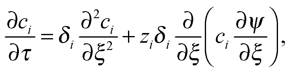
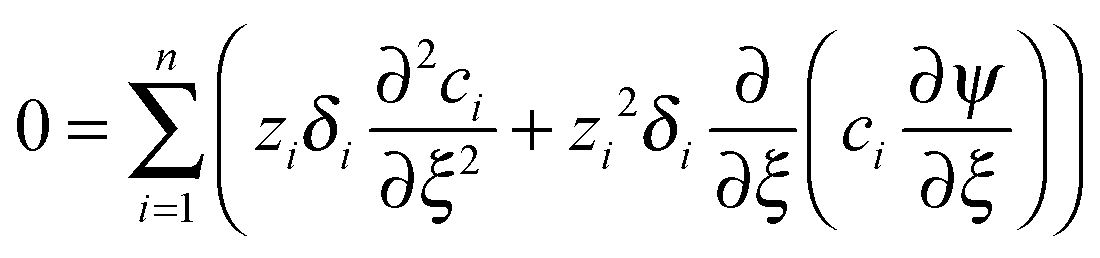
The conductometric cell can be considered one dimensional along its long axis. In this case the transport of ions can be described by the component and the charge balance equations according to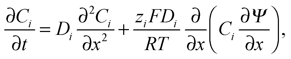 | (9) |
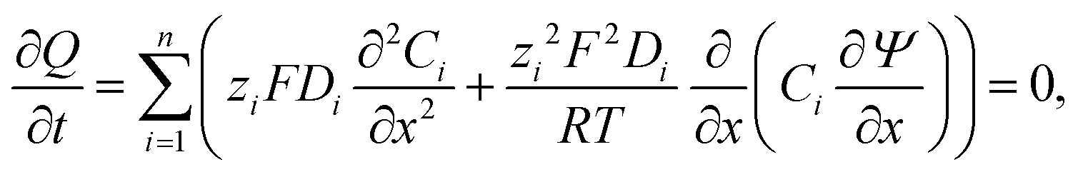 | (10) |
 | (11) |
 | (12) |
 ,
,  ,
,  , and
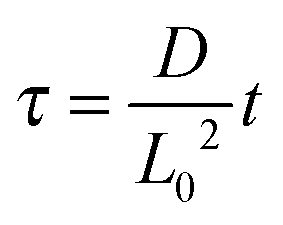
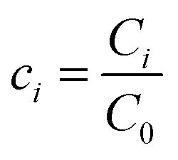
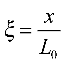
, and 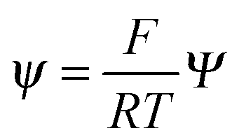 , where D is the diffusion coefficient of the diffusing anion, C0 is the input concentration of the diffusing electrolyte at one end, and L0 = 5 × 10⁻³ cm. One-dimensional spatial discretisation is then applied using the central difference formula for the first derivatives and the standard three-point Laplacian for the second derivatives. Introducing no-flux boundary conditions, the initial value problem defined by the discretised component balances is solved using backward differential formulae. The potential is calculated in each iteration step by solving the linear algebraic equation defined by the discretised charge balance.
The iterations are carried out on 12001 grid points with spatial resolution Δx = 0.1 using the CVODE package. The conductivity at each dimensionless coordinate is evaluated according to 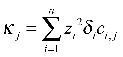 , then an average value is calculated around points ξ = 200 and ξ = 1000 corresponding to the locations of the electrodes. These average values (κtop and κbottom) are then used to obtain the effective diffusion coefficient by fitting
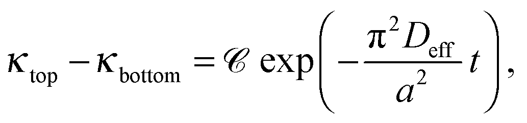
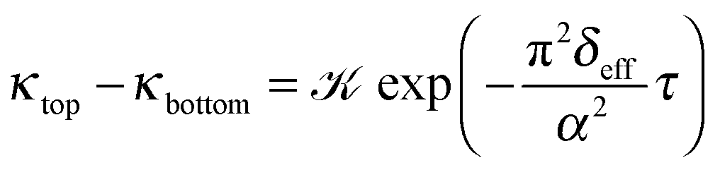 | (13) |
Two reference cases with different ratios of the diffusion coefficients of the cation and the anion have been selected for a binary electrolyte of ion charges z1 = 1 and z2 = −1. The first case with δ1 = 7, δ2 = 1 corresponds to the scenario in water where hydrogen ions can diffuse approximately seven times faster than other small ions due to the Grotthuss mechanism. The second case with δ1 = 3, δ2 = 1 anticipates the deceleration of the hydrogen ions in hydrogels compared to dilute solutions.
Calculations have been performed for a second set of conditions where a background electrolyte is introduced with a cation (z3 = 1, δ3 = 1) and an anion (z4 = −1 or −2, δ4 = 1 or 0). The last case with δ4 = 0 represents a hydrogel that contains bound anionic functional groups (e.g., carboxylate groups in gelatin). As initial conditions, the concentration profile of the ions of the main electrolyte is set according to c1 = c2 = 1 for ξ ≤ 10 and c1 = c2 = 0 for 10 < ξ ≤ 1200. Meanwhile, the relative concentration of the homogeneously distributed background electrolyte is varied as 10−1, 10−2, 10−3, 10−4, and 10−5 with respect to the input concentration of the main electrolyte at the boundary.
The temporal evolution of κtop and κbottom is presented in Fig. 2(a) for a selected case with no background electrolyte. The black dashed curve corresponding to the upper electrode near the area with high electrolyte concentration reveals an increase of conductivity caused by the incoming ions after the beginning of diffusion. After a short transient period, where κtop has a local maximum, the conductivity decreases due to the depletion of the zone. Meanwhile, κbottom increases thanks to the incoming ions of the diffusing electrolyte. Plotting (κtop–κbottom) versus the non-dimensional time depicts an exponential decay following a short transient period which is shown in Fig. 2(b) in a logarithmic form for easier visualisation. The δeff value of the main electrolyte can be obtained with the standard error of less than 0.01% using eqn (13). For the case of δ1 = 3 and δ2 = 1 we obtain 1.500, while for δ1 = 7 and δ2 = 1 we have 1.750 (without background electrolyte in both cases), indicating that these values are in excellent agreement with the theoretical ones obtained from eqn (7):  , respectively. Therefore, with the local input of the electrolyte in one end of the conductometric cell, the higher order Fourier terms indeed decay fast making eqn (4) valid. In addition, this also means that the conductivities at the ideal point locations preset according to the model can be replaced with the spatially averaged values relevant to experimental measurements.
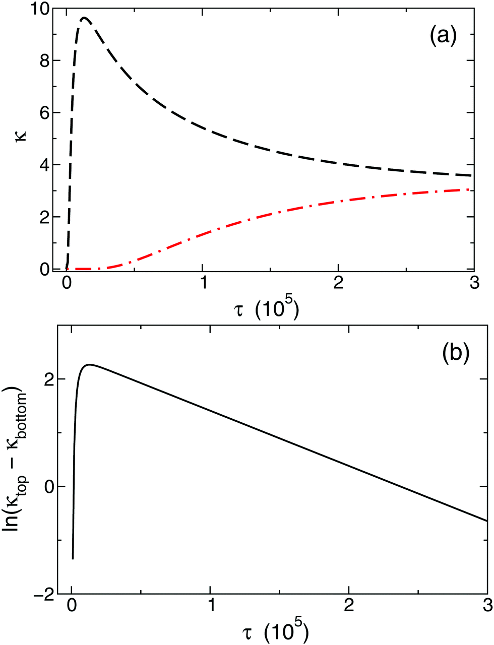 | ||
| Fig. 2 Temporal evolution of the calculated mean conductivity in the absence of background electrolyte at the top (black dashed curve) and bottom (red dashed and dotted curve) electrodes (a). Logarithm of the conductivity difference resulting in a linear correlation (b). | ||
Even though an exponential decay is still observed in the model introducing a background electrolyte with increasing concentration compared to the main electrolyte, the determined values for δeff exhibit an increasing deviation from those valid for pure binary electrolytes according to eqn (7). The influence of a background electrolyte can also be observed graphically as shown in Fig. 3. The resulting logarithmic curves for two different calculations are displayed where every parameter was kept constant except for the relative concentration of the background electrolyte. Therefore, a relative concentration exists, above which the exponential correlation required for eqn (13) becomes perceptibly distorted. The deviation from the ideal behavior can be tracked by changing the background electrolyte concentration provided that all other parameters are kept constant. Several values of δeff are listed in Table 1. After a systematic mapping of the parameters, we have found that the application of eqn (7) for calculating individual diffusion coefficients is acceptable for background electrolyte concentrations not more than 10−4 of the main diffusing binary electrolyte. This leads to an important experimental restriction, namely that in any experiment this large concentration difference has to be maintained to collect data applicable for evaluation.
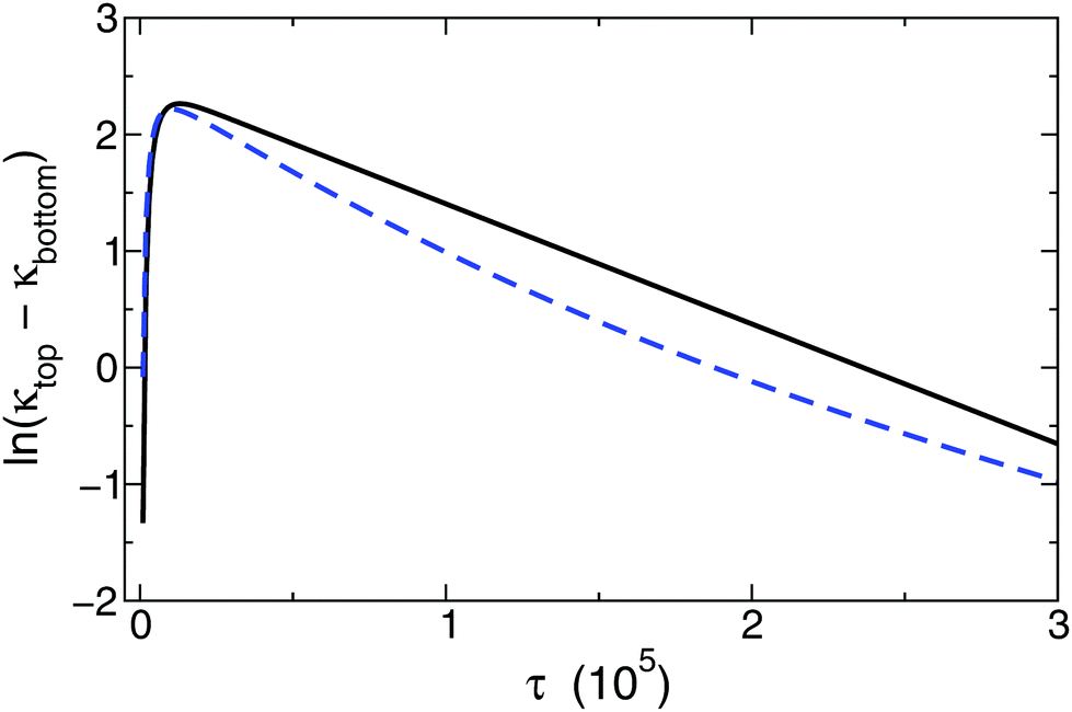 | ||
| Fig. 3 Graphical illustration of the impact of background electrolyte concentration on ionic diffusion. The black solid line represents a case when the relative concentration of the background electrolyte is low enough (10−4) to be negligible, meanwhile the blue dashed curve was acquired with a high concentration ratio (10−1) resulting in distorted correlation. | ||
| c b | δ eff |
|---|---|
| 10−5 | 1.499 |
| 10−4 | 1.491 |
| 10−3 | 1.356 |
| 10−2 | 1.092 |
| 10−1 | 1.019 |
4.2 Electric properties of the conductometric cell
In Harned and French's method, the conductance and hence conductivity values expressed at an distance from top and bottom of the cell are used for evaluation. In our custom-made cell, the electrodes are centered at these locations; however, their 1 cm2 area is not negligible considering the concentration gradient developing during the experiments.
Solution of the differential form of Ohm's law for our custom-made cell reveals that the electric current patterns between the two electrode surfaces in a pair are close to ideal parallel forms and, therefore, average conductance measured this way may be validly used for obtaining effective diffusion coefficients.(for details see the ESI,† Section A)
5 Experimental
5.1 Sample preparation for impedance and conductance measurements
Our experiments designed to determine the diffusion coefficient of hydrogen ions were conducted in agarose hydrogel from which 2 w/v% samples were prepared in order to fill the 6 cm3 inner space of the conductometric cell. This setup (see Fig. 1) was used both for impedance (see ESI,† Section B) and conductance measurements.For gel preparation, analytical reagent agarose powder (VWR DNA Grade) was mixed with deionized water to create a 2 w/v% solution, then the mixture was stirred and heated in a covered beaker until boiling. The homogeneous solution was left to cool for a few minutes, with constant stirring, then filled into the conductometric cell. Finally, it was left to set at room temperature. Later, the inner space of the cell was closed airtight, the cell was assembled and placed in a thermostated container for at least 12 hours prior the initiation. Meanwhile, a separate 2 mm thick, 1 cm × 1 cm piece of agarose was also prepared using a Plexiglas frame. The separate piece of gel was immersed in either 1 M NaCl or HCl solution (Molar) for the same time and used later to initiate diffusion.
5.2 Conductance measurements
Conductance measurements have been carried out inside a thermostated container at 25 °C while temperature fluctuation is constantly monitored throughout the experiment. The cell is electrically connected to the conductometer through a relay allowing a switch between the top and bottom electrodes in order to avoid cross-currents arising while simultaneously measuring at both pairs. Each conductance measurement is initiated by reopening the cell and placing the small piece of gel impregnated by electrolyte solution on top of the 6 cm3 agarose already filled and set in the inner space of the conductometric cell. The cell is then closed again and placed in the thermostated container for 90 minutes to let the main diffusing electrolyte penetrate. When the allotted time is over, the small hydrogel piece is removed, the cell is resealed and the measurement is initiated. Conductance is recorded first at the top then, after a switch in the relay, at the bottom electrodes. After two-minute pause, the conductance is measured again in the same manner. This cycle is repeated over the next 3–5 days and the data are collected using a computer. (For the validation of conductance measurements in the custom-made cell see the ESI,† Section B.)5.3 PFGSE-NMR measurements
The gel preparation process for PFGSE-NMR samples is similar to that for conductance measurements. A 0.1 M NaCl solution is made prior to gel preparation with 10 v/v% D2O (heavy water) content instead of pure deionised water, and then used for making a 2 w/v% agarose mixture. After stirring and heating the solution, a preheated quartz NMR tube is filled with a small amount of the solution. Then the tube is closed and the gel is allowed to cool and set.PFGSE-NMR measurements are performed on a Bruker Avance DRX 500 MHz instrument tuned to 23Na nucleus at 25 °C. The spectral width is set to 4000 Hz while the added D2O is used for locking the signal. The LED (longitudinal eddy-current delay) pulse sequence is applied where δ pulse length for the gradient field is set to 22000 μs with Δ = 0.03 s and τ = 0 s delay times between pulses (see eqn (8)).
6 Results and discussion
In the previous sections, it has been shown that an exponential relationship based on eqn (13) may be used to determine effective diffusion coefficients of binary electrolytes via conductance measurements provided that the concentration of the background electrolyte present in the hydrogel is sufficiently small. In addition, it has also been shown that eqn (7) may be validly used for such conditions to derive individual diffusion coefficients. We have determined both the theoretical and experimental cell constants in satisfactory agreement. The custom-made conductometric cell working with alternating current has proved to deliver impedance data where ohmic resistance is the major component (see ESI†). These requirements listed enable us to link together all experimental results and come to the final conclusions.For each recorded conductance value, conductivity is calculated using the experimental cell constants Ctop and Cbottom. Conductance measurements are evaluated using the dimensional form of eqn (13) as
 | (14) |
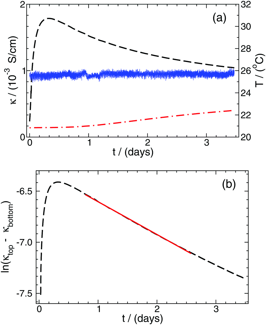 | ||
| Fig. 4 Conductivity (κ), calculated from the measured conductance and the appropriate cell constant, as a function of time at the top (black dashed curve) and bottom (red dashed and dotted curve) electrode pairs, respectively (a). The thickness of the line connecting the data points is greater than the fluctuations in the conductivity due to the 0.5% precision of the measurements. The solid blue curve represents the temperature recorded throughout the experiment. The logarithm of the conductivity difference between the two electrode pairs as a function of time (b). The solid red line represents the function fitted to the most appropriate time interval according to eqn (14). | ||
To determine the effective diffusion coefficient of the actual electrolyte, the function in eqn (14) is fitted to the data set obtained over a two-day period; its linearised form is presented in Fig. 4(b) for easier visualisation. This example case shows that an exponential decay is recovered in the experiments in good agreement with the theory detailed earlier. The effective diffusion coefficients Deff for NaCl and HCl electrolytes are calculated as an average of two or three parallel measurements given that a = 6 cm. Then, from PFGSE-NMR measurements, an individual value for the diffusion coefficient of Na+ ions is obtained using the Stejskal–Tanner equation (eqn (8)) for exponential curve-fitting. By applying eqn (7) twice – first for DNa+ and Deff,NaCl to obtain DCl−, then a second time for DCl− and Deff,HCl to obtain DH+ – the final individual diffusion coefficients of Cl− and H+ ions are determined in 2 w/v% agarose hydrogel. All those results are summarized in Table 2.
| Diffusion coefficient | Value (10−5 cm2 s−1) |
|---|---|
| D eff,NaCl | 1.640 ± 0.001 |
| D eff,HCl | 3.141 ± 0.002 |
| D Na+ | 1.35 ± 0.02 |
| D Cl− | 2.10 ± 0.04 |
| D H+ | 6.22 ± 0.37 |
The effect of a hydrogel medium on the diffusion of electrolytes and single ions can be concluded from our results as follows. In agarose, the mobility of simple ions such as Cl− and Na+ does not decrease significantly compared to their diffusion coefficients measured in dilute aqueous solutions (Deff,NaCl = 1.586 × 10⁻⁵ cm2 s−1 taken from the results of Harned and Hildreth37), which implies that they can freely diffuse in the high water content of the hydrogel. This also shows that there is no significant charge on the polymeric chain of the gel. However, the eventual DH+ value is only 3–4 times greater than the coefficients of other small ions, which supports the idea that, due to structural interactions between the polymer chain and the diffusing ions, the movement of hydrogen ions is hindered. It is probable that the spatial arrangement of polymer chains interferes with the hopping protons and thus reduces the efficiency of the Grotthuss mechanism. In hydrogels containing counterions, the polyelectrolyte backbone can further hinder the diffusion of hydrated hydrogen ions.41 It is our intention to further investigate the diffusion of hydrogen ions (and possibly the hydroxide ion as well) in such hydrogels that are widely used in the studies of chemical pattern formation and other applications listed in Section 1.
7 Conclusion
The diffusion coefficient of hydrogen ion in hydrogels plays an important role in many research activities, e.g. in reaction–diffusion pattern formation, pH responsive gels, pH-regulated self-healing mechanisms, and in hydrogels used for drug delivery. Their values, however, have only been approximated lacking a method that can directly deliver the relevant data. Here we have presented a complex but reproducible experimental procedure based on conductance and PFGSE-NMR measurements to gain access to the desired diffusion coefficient. With modeling calculations we have also shown that this general method can be extended to determine the relevant diffusion coefficients of the hydrogen ion in different hydrogel media.Acknowledgements
This work was supported by the National Research, Development and Innovation Office (K119795) and GINOP-2.3.2-15-2016-00013 projects. G. Schuszter also thanks the National Research, Development and Innovation Office (PD121010), while T. Gehér-Herczegh thanks ESTEC/4000102255/11/NL/KLM for the financial support.References
- Q. Ouyang and H. L. Swinney, Nature, 1991, 352, 610–612 CrossRef.
- J. Horváth, I. Szalai and P. De Kepper, Science, 2009, 324, 772–775 CrossRef PubMed.
- I. Szalai and P. De Kepper, Comm. Pure & Appl. Anal., 2012, 11, 189–207 Search PubMed.
- J. E. Pearson, Science, 1993, 261, 189–192 CAS.
- K.-J. Lee, W. D. McCormick, J. E. Pearson and H. L. Swinney, Nature, 1994, 369, 215–218 CrossRef.
- Z. Virányi, I. Szalai, J. Boissonade and P. De Kepper, J. Phys. Chem. A, 2007, 111, 8090–8094 CrossRef PubMed.
- I. Molnár and I. Szalai, J. Phys. Chem. A, 2015, 119, 9954–9961 CrossRef PubMed.
- I. Szalai, J. Horváth, N. Takács and P. De Kepper, Phys. Chem. Chem. Phys., 2011, 13, 20228–20234 RSC.
- A. Hanna, A. Saul and K. Showalter, J. Am. Chem. Soc., 1982, 104, 3838–3844 CrossRef CAS.
- D. Horváth and A. Tóth, J. Chem. Phys., 1998, 108, 1447–1451 CrossRef.
- M. Fuentes, M. N. Kuperman and P. De Kepper, J. Phys. Chem. A, 2001, 105, 6769–6774 CrossRef CAS.
- M. Dayeh, M. Ammar and A. G. Mazen, RSC Adv., 2014, 4, 60034–60038 RSC.
- I. Szalai, J. Phys. Chem. A, 2014, 118, 10699–10705 CrossRef CAS PubMed.
- I. Varga, I. Szalai, R. Mészaros and T. Galányi, J. Phys. Chem. B, 2006, 110, 20297–20301 CrossRef CAS PubMed.
- T. Ueki and R. Yoshida, Phys. Chem. Chem. Phys., 2014, 16, 10388–10397 RSC.
- L. Roszol, T. Lawson, V. Koncz, Z. Noszticzius, M. Wittmann, T. Sarkadi and P. Koppa, J. Phys. Chem. B, 2010, 114, 13718–13725 CrossRef CAS PubMed.
- L. Roszol, A. Várnai, B. Lorántfy, Z. Noszticzius and M. Wittmann, J. Chem. Phys., 2010, 132, 064902 CrossRef CAS PubMed.
- Y. Qiu and K. Park, Adv. Drug Delivery Rev., 2001, 53, 321–339 CrossRef CAS PubMed.
- T. Manouras and M. Vamvakaki, Polym. Chem., 2017, 8, 74–96 RSC.
- V. Yesilyurt, J. M. Webber, E. A. Appel, C. Godwin, R. Langer and D. G. Anderson, Adv. Mater., 2016, 28, 86–91 CrossRef CAS PubMed.
- Y. Yang and W. M. Urban, Chem. Soc. Rev., 2013, 42, 7446–7467 RSC.
- Y. Zhu, H. Xuan, J. Ren and L. Ge, Soft Matter, 2015, 11, 8452–8459 RSC.
- I. Lagzi and D. Ueyama, Chem. Phys. Lett., 2009, 468, 188–192 CrossRef CAS.
- I. Lagzi, Langmuir, 2012, 28, 3350–3354 CrossRef CAS PubMed.
- W. Dyck, Can. J. Chem., 1971, 49, 1575–1578 CrossRef CAS.
- A. Pluen, P. A. Netti, R. K. Jain and D. A. Berk, Biophys. J., 1999, 77, 542–552 CrossRef CAS PubMed.
- M. Golmohamadi and K. J. Wilkinson, Carbohydr. Polym., 2013, 94, 82–87 CrossRef CAS PubMed.
- C. Mattisson, P. Roger, B. Jönsson, A. Axelsson and G. Zacchi, J. Chromatogr. B: Biomed. Sci. Appl., 2000, 743, 151–167 CrossRef CAS.
- S. Liang, J. Xu, L. Weng, H. Dai, X. Zhang and L. Zhang, J. Controlled Release, 2006, 115, 189–196 CrossRef CAS PubMed.
- P. Lundberg and P. W. Kuchel, Magn. Reson. Med., 1997, 37, 44–52 CrossRef CAS PubMed.
- E. O. Stejskal and J. E. Tanner, J. Chem. Phys., 1965, 42, 288–292 CrossRef CAS.
- C. S. Johnson, Jr., Prog. Nucl. Magn. Reson. Spectrosc., 1999, 34, 203–256 CrossRef.
- H. Harned and D. French, Ann. N. Y. Acad. Sci., 1945, 44, 267–281 CrossRef.
- H. Harned and R. Nuttall, J. Am. Chem. Soc., 1947, 69, 736–740 CrossRef CAS PubMed.
- H. Harned and R. Nuttall, J. Am. Chem. Soc., 1949, 71, 1460–1463 CrossRef CAS.
- H. Harned and C. Blake, J. Am. Chem. Soc., 1950, 72, 2265–2266 CrossRef CAS.
- H. Harned and C. H. Jr, J. Am. Chem. Soc., 1951, 73, 650–652 CrossRef CAS.
- H. Harned and R. Hudson, J. Am. Chem. Soc., 1951, 73, 3781–3783 CrossRef CAS.
- Z. Virányi, Á. Tóth and D. Horváth, J. Eng. Math., 2007, 59, 229–238 CrossRef.
- Z. Virányi, Á. Tóth and D. Horváth, Phys. Rev. Lett., 2008, 100, 088301 CrossRef PubMed.
- F. Bordi, C. Cametti and G. Paradossi, J. Phys. Chem., 1991, 95, 4883–4889 CrossRef CAS.
Footnotes |
| † Electronic supplementary information (ESI) available. See DOI: 10.1039/c7cp00986k |
| ‡ These authors contributed equally to the work. |
| This journal is © the Owner Societies 2017 |