Local pH and effective pKA of weak polyelectrolytes – insights from computer simulations†
Received
13th January 2017
, Accepted 28th February 2017
First published on 28th February 2017
Abstract
In this work we study the titration behavior of weak polyelectrolytes by computer simulations. We analyze the local pH near the chains at various conditions and provide molecular-level insight which complements the recent experimental determination of this quantity. Next, we analyze the non-ideal titration behaviour of weak polyelectrolytes in solution, calculate the effective ionization constant and compare the simulation results with theoretical predictions. In contrast with the universal behaviour with respect to chain length, we find non-universality and deviations from theory with respect to polymer concentration and permittivity of the solvent. The latter we explain in terms of counterion condensation and ion correlation effects, which lead to reversal of the non-ideal titration behaviour at very low permittivities. We discuss the impact of these findings on the interpretation of experimental results.
1 Introduction
Ionizable groups in weak polyelectrolytes are weak acids or bases, and their ionization is variable in response to changes in the environment. This is in contrast with strong polyelectrolytes, ionization of which is fixed at the time of synthesis. Compared to low molar mass weak acids and bases, dissociation of weak polyelectrolytes is much more complex. The electrostatic interaction between the nearby ionized groups on the chain provides an additional conformation-dependent free energy cost of ionization. Therefore ionization of weak polyelectrolytes is suppressed as compared to the corresponding monomer. In addition, the increased ionization of the macromolecule brings about expansion of its conformation, and changes in the distribution of counter-ions and of other small ions around the chain.
The variable ionization of weak polyelectrolytes is being exploited in various pH-responsive polymer systems. For example, the pH-dependent self-assembly and gelation of diblock copolymers1–3 and of gradient copolymers4,5 containing poly(acrylic acid), pH-responsive swelling and collapse of polymer-coated nanoparticles,6 polyelectrolyte microgels7,8 and co-networks.9,10 However, in most experimental works the interpretation of pH-responsive behaviour of weak polyelectrolytes is based on intuitive extrapolation of the textbook knowledge about ionization of simple weak acids. For example, it is commonly assumed that at pH > pKA + 1 the acid is almost fully ionized. This is true for low-molecular acids while polyelectrolytes hardly reach 50% ionization under such conditions.
In this work we use computer simulations to unravel some of the non-trivial features of the non-ideal ionization of weak polyelectrolytes in solution. We address the local effects that arise as a consequence of coupling between ionization and conformation of the polyelectrolyte. We also address the changes in titration curves of the polyelectrolyte with varying chain length, polymer concentration, and solvent permittivity.
2 Theoretical background
2.1 Thermodynamics of acid–base equilibria
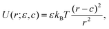
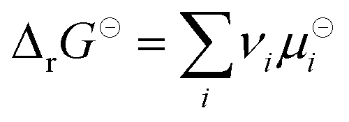
Some well-known terms from theory of acid–base equilibria attain non-trivial meanings in nano-heterogeneous systems, such as polyelectrolyte solutions. Therefore we briefly review here the key points of the theory, emphasizing the connection to polyelectrolytes. For simplicity, we restrict further discussion to weak polyacids, keeping in mind that analogous arguments apply to polybases. Consider the schematic ionization reaction of a weak acidic group A| | HA ![[left over right harpoons]](https://www.rsc.org/images/entities/char_21cb.gif) A− + H+. A− + H+. | (1) |
The reaction equilibrium in eqn (1) is characterized by the acidity constant KA, or its negative logarithm pKA = −log10![[thin space (1/6-em)]](https://www.rsc.org/images/entities/char_2009.gif) KA, which is related to the chemical potentials as
KA, which is related to the chemical potentials as| | 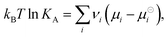 | (2) |
where  is the standard Gibbs free energy change of the reaction, νi is the stoichiometric coefficient and μi the chemical potential of species i participating in the reaction. The chemical potential can be further written in terms of activity
| | 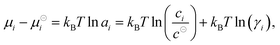 | (3) |
where μ⊖i is the reference (standard) chemical potential, ai is the activity, ci is the concentration, γi is the activity coefficient of species i. The reference concentration c⊖ is given by the choice of the reference state. We can further split the chemical potential to the ideal gas term, μidi, and the excess term, μexi, which accounts for the influence of interactions:| | | μidi = kBTln(ci/c⊖), μexi = kBTln(γi). | (4) |
It is convenient to characterize ionization in terms of the degree of ionization – the ratio of the amount of the ionized form and the total amount of the given species,
Substituting from
eqn (5) and (3) to
eqn (2) and assuming ideal behaviour (
γ = 1), we obtain the
ideal titration curvewhich well describes ionization of simple low-molar-mass acids up to
c ≈ 0.1 M.
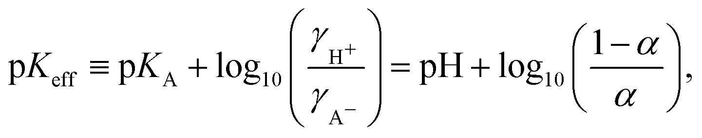
Eqn (6) is often used as the defining relation for the effective acidity constant, p
Keff11–13| |  | (7) |
which can be calculated from the experimentally measured
α. Because p
Keff implicitly includes all the non-idealities, it is not a true constant but exhibits a non-trivial dependence on all relevant parameters, such as the degree of ionization, polymer chain length, polymer concentration and salt concentration.
12,14,15 Consequently, it characterizes one particular state of the system under one specific set of conditions. Although the use of
Keff is convenient from practical view of analyzing experimental data, it only provides limited information for understanding of the underlying phenomena and for predictions of behaviour under different conditions.
2.2 The definition of pH
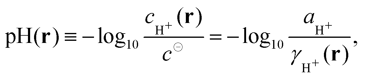
In eqn (7) we have assumed the following definition of pH| |  | (8) |
which allows us to use the term “local pH” as it is commonly used in literature to describe local variations in cH+(r) in nano-heterogeneous systems. To emphasize this, we have explicitly written the relevant quantities in eqn (8) as a function of the position vector r. Local pH is often invoked to explain deviations from the ideal behaviour but it is very difficult to measure. Nevertheless, it has been recently measured for a single polyelectrolyte chain and for a star-like polyelectrolyte in solution by means of single-molecule fluorescence techniques.16–18
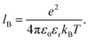
In this context it is noteworthy that historically the pH has been first defined by means of concentration of H+ ions,19 and only later it has been defined by means of the activity.20,21 The present operational definition21 relies on a convention based on the electromotive force on the hydrogen (or glass) electrode, such that it can be reproducibly measured and is close to −log10aH+.20 Note that the chemical potential and activity are constants throughout the whole system, and do not vary locally under equilibrium. If there are local variations of concentration, these have to be compensated by local variations of the activity coefficient, as is implied by eqn (3) and (8). Note that if pH should be defined as the logarithm of activity, rather than concentration, it implies that at equilibrium pH is constant in the whole system, and the term “local pH” would become essentially meaningless. In further text, we will use the term local pH for pH in the immediate vicinity of the chain (see section Local pH and bulk pH for more precise definition). By bulk pH we will refer to pH far from the chain, where the influence of the polyelectrolyte is minimal.
2.3 Theory of ionization of weak polyelectrolytes
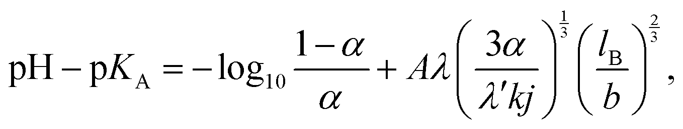
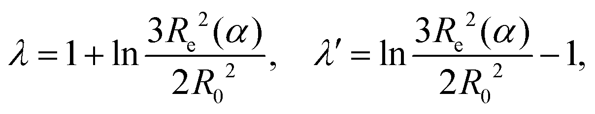
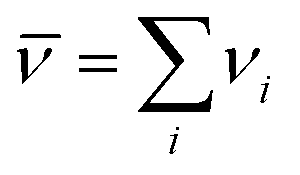
Theoretical attempts to predict the ionization degree of a weak polyelectrolyte as a function of its molecular weight, concentration, solution pH, or permittivity can be tracked back to the seminal work of Katchalsky and Gillis.14 Within the Debye–Hückel approximation for electrostatic interaction, assuming charges homogeneously distributed along the chain, and neglecting correlations with counterions they derived the following equation:| | 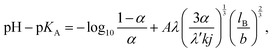 | (9) |
where lB is the Bjerrum length defined in eqn (13), b is the bond length, A = 2(4π)2/3ln(10) is a constant pre-factor, k is the number of monomers per Kuhn segment, and 1/j is the fraction of monomers of the polymer capable of ionization. The parameters λ and λ′ are defined as| | 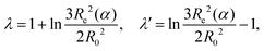 | (10) |
where Re and R0 are the end-to-end distances of the ionized chain, and of the neutral chain, respectively. Katchalsky and Gillis in their work neglected the interaction between the ionized macromolecules and their counterions and also between different chains. Therefore their theory cannot predict the concentration dependence of the ionization and it should fail at high concentrations and above the Manning condensation threshold. However, as follows from the discussion below, it qualitatively well describes the experimentally observed trends in ionization of polyelectrolytes in a rather broad range of parameters.
Eqn (9) can be further simplified, realizing that λ and λ′ vary very slowly with α or N. If they are assumed constant, we obtain an explicit relation for the dependence of pKeff on α
| | | pKeff(α,N,…) = pKA + m(N,…)α1/3u2/3, | (11) |
where
u =
lB/
b is the dimensionless electrostatic coupling parameter, and
m is a weakly varying function of all other parameters, which can be determined by fitting experimental data. If both
m and p
KA are treated as adjustable parameters,
eqn (11) well represents experimental data for poly(acrylic acid) at low concentrations in salt-free solutions, and the obtained values of
m and p
KA slightly vary with polymer concentration.
12 This variation of p
KA reflects the fact that the theory behind
eqn (9) does not explicitly account for the influence of counterions, or for interactions between individual polymer chains. Interestingly, for the more hydrophobic poly(methacrylic acid), the use of
eqn (11) fails even on the qualitative level.
12 Presumably this is because hydrophobic polyelectrolytes exhibit domain formation
22,23 which was not considered in the original theory.
Raphael and Joanny24 have been able to predict the local variation of the degree of ionization, α(s), with the monomer position in the chain, s, as a function of the average degree of ionization, α. Their prediction is in excellent agreement with our recent simulation results,25 however, it does not predict how α depends on the properties of the polymer, or of the solution.
Over the years many other phenomenological approaches to predictions of the ionization of weak polyelectrolytes have appeared in literature. However, often the physical meaning of their parameters is not straightforward, or they do not provide a simple analytical relation but require numerical solution of the equations, as discussed in ref. 26 for the special case of poly(acrylic acid). A handful of simulation studies dealing with various aspects of weak polyelectrolytes can also be found in literature. A comprehensive overview can be found in reviews.26–28 Below we address some selected papers relevant for further discussion. Early simulations of weak polyelectrolytes have focused on the role of chain length in ionization, and comparison with the universal titration curve.29–31 About two decades later, Panagiotopoulos investigated in simulations the role of electrostatic coupling.32 Uyaver and Seidel have investigated the collapse of weak polyelectrolytes under poor solvent conditions33,34 and the nonuniform charge distribution along the chain35 within the Debye–Hückel approximation. The same approximation has been used by Ullner and Jönsson,36,37 and by Ulrich et al. to study conformation changes with ionization38 and by Carnal et al. to study adsorption of weak polyelectrolytes at nanoparticles.39 Other groups have investigated the behaviour of weak polyelectrolyte gels under various conditions.40–42 Ziebarth and Wang studied the changes of ionization of poly(ethylene imine) interacting with DNA.43,44 In all these studies one of the key aspects of the observed behaviour was the coupling between the conformation and ionization of the weak polyelectrolyte. However, investigation of the local pH near polyelectrolyte chain by means of computer simulations is lacking. Since the local pH in polyelectrolyte solutions has been measured in recent experiments,17,18,45,46 it is timely to investigate it in computer simulations and to contrast the experimental and simulation results. Similarly, the role of polymer concentration has not been investigated in computer simulations, while its influence on the titration behaviour of weak polyelectrolytes is evidenced in experiments.13 The above two aspects of weak polyelectrolyte behaviour are the subject of our present investigation.
3 Polymer model
The model and methodology employed in this study are identical to what has been described in our previous publications,25,47 therefore we restrict ourselves here to a brief description, and refer the reader to the earlier publications for additional details.
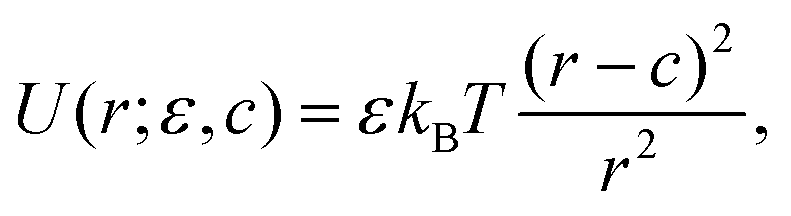
We employ a bead-spring model consisting of N monomers, where each monomer is modeled by a soft repulsive potential which corresponds to the athermal (good) solvent conditions:
| |  | (12) |
where
c and
ε are adjustable parameters which we set to
ε = 1.5
kBT, and
c = 2
b, where
b = 0.41 nm is the effective monomer size. Monomers are connected by harmonic springs with the equilibrium bond length
b, and the stiffness constant
k = 24.4
kBT nm
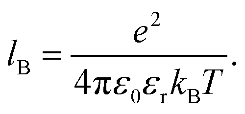
−1. The solvent is treated implicitly as a dielectric continuum with the given relative permittivity,
εr, and with the corresponding Bjerrum length:
| |  | (13) |
The charged particles interact
via Coulomb potentials and the electrostatic interaction energy is evaluated using the Ewald summation.
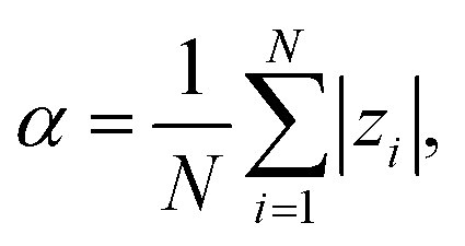
We define the degree of ionization of the chain, α, as the average over individual monomers:
| |  | (14) |
where
zi is the charge number of monomer
i in a particular state. The reported values of
α (and all other observables) are estimates of ensemble averages calculated over many system configurations. Each monomer is a weak acid, characterized by the ionization constant,
KA, which is the input parameter of the simulation. We carry out a series of simulations, systematically varying p
KA, which determines the value of
α. We would like to emphasize that we vary pH by means of varying the strength of the acid, the p
KA (see Section 4 for more details). No salt was added.
3.1 Parameters of the studied systems
Unless stated otherwise, we use the following default set of parameters: number of chains n = 1 of length N = 100 beads in a cubic simulation box with edge length L such that the monomer density cpol = nN/L3 ≈ 1.4 × 10⁻² mol l−1. We set the default permittivity to that of water at room temperature, εr = 80, which results in the electrostatic coupling u = lB/b ≈ 2. We systematically vary KA in different systems such that it covers the whole range of ionization degrees 0 < α < 1. To study the effect of molecular weight of the polymer, we vary the length between 1 < N < 200.
When studying the concentration effects, we vary the simulation box size such that the concentration of monomer units is in the range 1.4 × 10⁻² < cpol < 1.4 × 10⁻¹ mol l−1. For poly(acrylic acid) this corresponds to the usual concentration range used in experiments, 1.0–10.0 mg ml−1.
For the investigation of the role of solvent permittivity it is important to realize that, following eqn (9), the key control parameter is the dimensionless electrostatic coupling, u = lB/b. In our simulations b is fixed based on an estimate from the geometry of poly(acrylic acid), while for other polyelectrolytes the value could be different depending on the chemical structure. For example for poly(styrene sulfonate) distance between the charged groups is about 1 nm because they are attached to a rather bulky side-group.48 Such details are below the resolution of the coarse-grained model, but should be considered when comparing simulation results to experiments. Therefore comparison of simulations with experiments should always be done for the given value of u, rather than b or εr alone. For example the case of poly(styrene sulfonate) in water with lB/b ≈ 0.7 could be mapped on our simulation results with εr ≈ 140 and b = 0.41 nm. To allow for such mapping we vary the permittivity in the range 17 < εr < 293 which goes slightly beyond the highest available permittivities of real solvents, εr ≈ 180.49 It should be noted that such re-scaling of electrostatic interactions neglects the excluded volume effects due to finite size of ions and of the polymer segments. In most situations considered here, the excluded volume is negligible because typical distances between ions are much greater than their own size. Only beyond the Manning condensation threshold, when many counterions are condensed, the excluded volume contribution may become important and render the above-described mapping inapplicable.
To rule out possible artifacts of periodic boundary conditions and finite size effects due to small number of chains in the box, for selected systems we compared simulations with n = {1, 3, 5, 10} chains per simulation box, adjusting the box volume such as to keep the polymer concentration constant. In most cases, the results were rather insensitive to the number of chains in the box, the differences being smaller than the estimated statistical error (see Fig. S1 of the ESI,† for details). In some cases, however, we observed significant differences. These are addressed in the respective parts of Results and discussion.
4 Simulation methodology
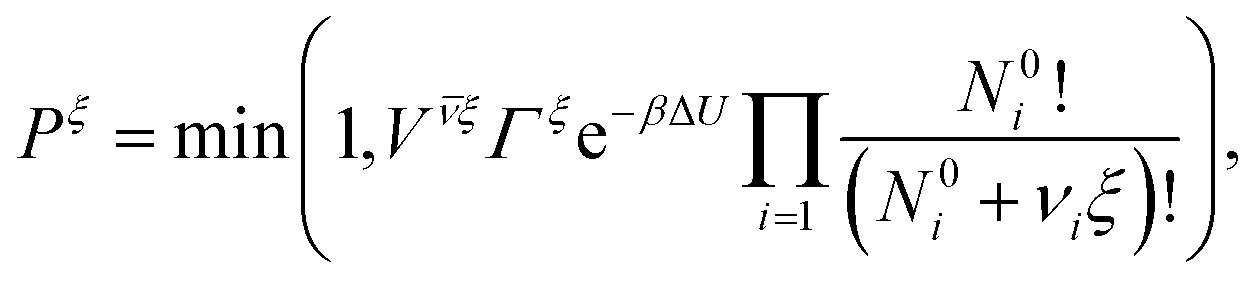
To account for the ionization reaction we employ the reaction ensemble,50 and to sample the configuration space we use a variant of the hybrid Monte Carlo (HMC) method51 particularly suitable to polymer systems.52 In each HMC step we perform either a conformation move, or a reaction move. In the conformational move the new state is obtained by a dynamical time evolution as in the usual molecular dynamics (except for using a modified evolution Hamiltonian52), and the trial configuration thus obtained is accepted or rejected using the Metropolis criterion (with the original Hamiltonian). The freely adjustable parameters (time step, trajectory length, etc.) are optimized to minimize the number of force evaluations per one independent sample of radius of gyration of the chain. The optimum is a compromise between faster evolution and better energy conservation entering the Metropolis criterion. It allows for much longer time-steps than in ordinary molecular dynamics while still exactly sampling the Boltzmann distribution. In the reaction move we select with equal probabilities the forward or reverse direction of the reaction in eqn (1). In the forward direction a randomly selected non-ionized monomer becomes ionized, and an H+ ion is inserted at a random position in the box. In the reverse direction a randomly selected ionized monomer is de-ionized, and a randomly selected H+ ion is removed. The acceptance probability Pξ for move from state o to n in the reaction ensemble is given by the criterion:50| | 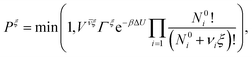 | (15) |
where ΔU = Uo − Un is the interaction energy change, 1/β = kBT, V is the simulation box volume,  , and νi is the stoichiometric coefficient of species i in the reaction eqn (1) (negative for the reactants and positive for the products). The instantaneous number of species i in the simulation box, Ni is linked to its the initial number, N0i through the extent of reaction, ξ:Finally, Γ is related to KA as
| | 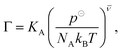 | (17) |
where NA is the Avogadro number and p⊖ = 1 atm is the arbitrarily chosen standard pressure. At low densities considered here this simple method without any bias is sufficiently efficient. A detailed description can be found in our previous work.25
4.1 Simulation protocol and data analysis
Starting from an arbitrary polymer conformation, we first perform an equilibration run which is discarded from further analysis, followed by a longer production run which is used for sampling and collection of data. Duration of a typical simulation is 105 configuration moves and about the same number of reaction moves. Per configuration move, we perform an MD simulation run of about 50 time steps. The HMC method yields correct ensemble averages irrespective of the choice of the above parameters, however, their values dramatically influence the efficiency of sampling. The optimum parameter range is relatively narrow and system-dependent, therefore it needs to be determined by tuning.
To characterize the quality of our data, we use the method of Wolff53 to estimate the number of statistically independent samples. Our typical productive run generates about 104 uncorrelated samples of Rg, which turns out to be the slowest evolving studied observable. The evolution of some systems (low εr, large N, low or high α) was slower, so that it was difficult to obtain the desired number of uncorrelated samples. We consider 103 uncorrelated samples as a threshold below which the simulations were not credible. In the reaction ensemble it is necessary to ensure that both the ionization and the polymer conformations are sampled properly by tuning the reaction step probability so that ideally the autocorrelation times of α and Rg are comparable. In practice, the reaction step is computationally much cheaper than the conformational move, therefore we prefer to oversample the reaction using a higher reaction probability. Then the overall quality of the simulation can be assessed on the basis of the slower conformational evolution alone at the cost of small computational overhead.
5 Results and discussion
5.1 Local pH and bulk pH
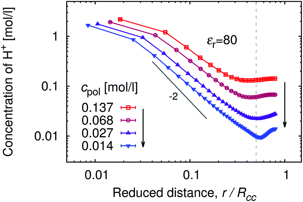
In Fig. 1 we show the density profiles of H+ ions around the polymer chain with α ≈ 1, as a function of distance from the middle monomer for a series of polymer concentrations. The distance in Fig. 1 is scaled by the typical separation between the chains, Rcc, which can be estimated as Rcc = (3N/4πcpol)1/3. As a general trend, the concentration profiles initially decay with the power law close to the theoretical prediction c(r) ∼ r−2 for star-like polyelectrolytes.54 The same power law is even more closely followed by the segment density profile (see ESI,† Fig. S2), indicating uniformly stretched chains. A qualitative difference shows up at higher separations, where the segment density profiles rapidly drop to unity while H+ profiles level off in the intermediate region between the chains. Fig. 1 shows profiles obtained with 5 chains in the box in order to demonstrate that in this region the profiles pass through a minimum which corresponds to half of the maximum separation between two chains. Then they increase again as the distance approaches typical separation between two chains, with the highest probability of finding another polymer chain (for better illustration, see also simulation snapshot in the ESI,† Fig. S9). In principle, we should observe further oscillations of the concentration profile with decreasing amplitude, similar to the shape of radial distribution functions of simple liquids. However, this would require far more chains in the simulation box than we can conveniently handle. Notably, the difference between cH+ near the chain and in the bulk (minimum of cH+(r)), makes a factor of ≈5 for the high polymer concentrations cpol ≈ 1.4 × 10⁻¹ mol l−1, and a factor of ≈50 for the low polymer concentrations cpol ≈ 1 × 10⁻² mol l−1.
 |
| | Fig. 1 Proton concentration as a function of distance from the central monomer r, scaled by the average separation between the chains Rcc, obtained with 5 chains per simulation box for fully ionized chains with KA = 10, (α = 1), solvent permittivity εr = 80 and a series of polymer concentrations, cpol, given in the legend. The vertical dashed line marks the distance where r/Rcc = 1/2. | |
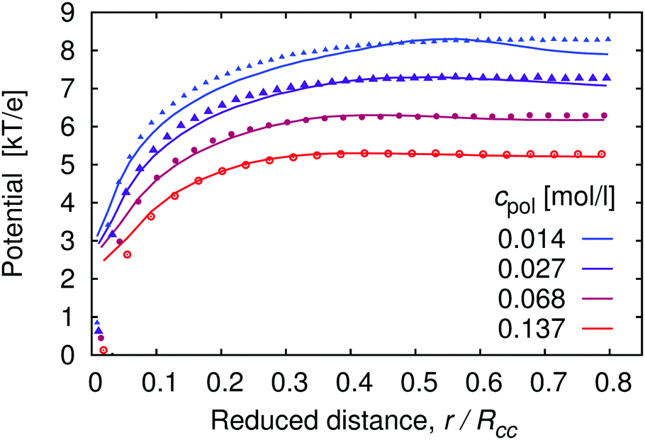
The concentration profiles of H+ ions are determined by the potential of mean force, Ũ(r), which is the effective interaction felt by an ion at a given position, averaged over positions of all other particles in the system.55Ũ(r) is defined as the negative logarithm of the pair correlation function, g(r), and can be approximated by the mean electrostatic potential, 〈Ψ(r)〉. For the distribution of H+ ions around the chain we have g(r) ∼ cH+(r), hence (up to an arbitrary additive constant)
| | Ũ(r) = −kBT![[thin space (1/6-em)]](https://www.rsc.org/images/entities/i_char_2009.gif) ln(〈cH+(r)〉) ≈ 〈Ψ(r)〉. ln(〈cH+(r)〉) ≈ 〈Ψ(r)〉. | (18) |
The approximation
Ũ(
r) ≈ 〈
Ψ(
r)〉 has been used in recent experimental works to determine the local electrostatic potential near a polyelectrolyte chain from the measured local concentration of H
+ ions.
16–18 In simulations we can explicitly calculate 〈
Ψ(
r)〉 by inserting a test charge and a homogeneously distributed background charge,
56,57 and averaging over different configurations. At the same time, we can calculate
Ũ(
r) from the concentration profiles shown in
Fig. 1. The comparison of
Ũ(
r) and 〈
Ψ(
r)〉 in
Fig. 2 shows very good agreement almost in the whole range. There is a slight disagreement at separations corresponding to the maximum probability of finding another chain, around
r/
Rcc = 1/2. Here
Ũ(
r) exhibits a weak maximum which is most visible at the lowest concentration, while 〈
Ψ(
r)〉 is quite flat. Around
r =
Rcc the angular dependence of 〈
Ψ(
r)〉 is very strong: deep minima in very localized positions where the other chains are found, flat maxima elsewhere. With strong angular correlations, the mean-field averaging over angular coordinates is not well applicable. Another disagreement occurs at very small values of
r ≤
σ where the short-ranged excluded volume interaction dominates over electrostatics. However, for the experimental estimation of 〈
Ψ(
r)〉 from the local proton concentration the relevant quantity is the difference 〈
ψ(
σ)〉 − 〈
ψ(
Rcc/2)〉, in which case the above-discussed differences are quite inconsequential. Therefore we can conclude that the recent experiments
16–18 provide a very good approximation the true value of 〈
Ψ(
r)〉.
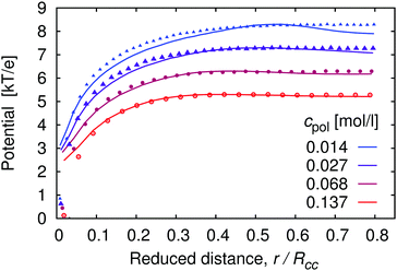 |
| | Fig. 2 Effective potential felt by H+ ions as a function of distance from the central monomer r, scaled by the average separation between the chains Rcc, for the same systems as in Fig. 1. Points represent the mean electrostatic potential 〈Ψ(r)〉, curves represent the potential of mean force Ũ(r) (see eqn (18)). We add an arbitrary constant to each potential such that the maxima of the corresponding potentials at the same cpol attain the same value. | |
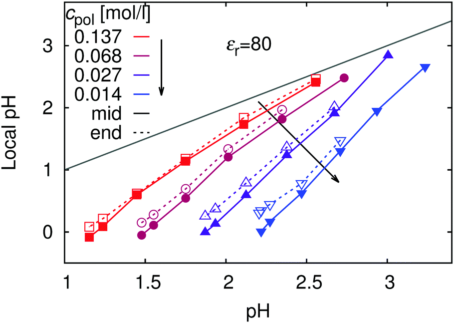
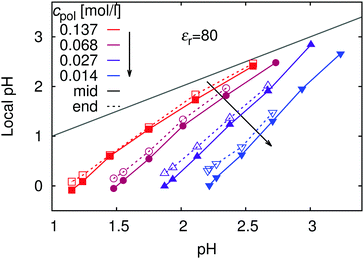
As discussed in the section Theoretical background, the concentration of H+ ions in the vicinity of the chain determines the local pH, while cH+ far away from the chain (at the minimum of the cH+(r) dependence) determines the bulk pH or simply pH (i.e., the value that would be measured by a conventional pH meter). For the local pH near the chain we use the maximum of the cH+(r) dependence, which typically occurs within r ≲ 2b. Since our definition of local pH is arbitrary, we performed a sensitivity analysis to demonstrate that various plausible definitions yield very similar results (see ESI,† Fig. S3). Fig. 3 shows that local pH is always lower than the bulk pH. At this point it is important to recall that in our simulations all the H+ ions come from the polyelectrolyte ionization and the different pH values are attained by means of varying the pKA. Therefore low pH corresponds to high ionization and high pH corresponds to low ionization. In an experiment where one would use a polymer with a fixed pKA and control pH by a buffer, the situation would be reversed.
 |
| | Fig. 3 Local pH (see eqn (8) for definition) in the vicinity of the chain: in the middle of the chain (full symbols) and at the end (empty symbols), as a function of pH in the bulk for various polymer concentrations, cpol. The grey line marks the values where both quantities are equal. Estimated errors are smaller than the symbol size. | |
The biggest differences between the bulk and local pH occur when the polymer is fully ionized, while with decreasing ionization (increasing pH) the local and bulk pH approach each other. In terms of proton concentration, this means that cH+ in the vicinity of the fully ionized chain is much higher than in the bulk. As the ionization of the chain decreases (increasing pH), influence of the chain on the concentration profile becomes weaker, and local pH approaches the bulk value. This observation is consistent with existing experimental observations for the cationic poly(2-vinyl pyridine).18,46 In addition, our simulations show that the difference between the bulk and local pH significantly diminishes with increasing polymer concentration (Fig. 3) and increases with chain length (ESI,† Fig. S3). The concentration dependence of ionization can be understood by comparison with the concentration-dependence of profiles of H+ ions in Fig. 1. With increasing dilution, the volume per chain increases, and counterions are distributed over the whole volume, while the chain connectivity restricts the volume in which ionized segments are confined.
Fig. 3 also reveals a small but still measurable increase in local pH when going from the middle of the chain (i.e., central monomer) toward the end (terminal monomers). This decrease in the concentration of counterions around the ends of polyelectrolyte chain has been termed end-effect.58 Similar trend was observed in experiments on star-like polyelectrolytes.18 Thanks to the higher molecular weight and star-like nature of the polymer the experimentally observed difference between the middle and the end was more pronounced (about 0.3 units of pH) than in our simulations. However, our present results cannot explain the relation between the local and bulk pH in the strong poly(styrene sulfonate),17,45 where the ionization is independent of pH and the mechanism behind the local pH variation is presumably different.
5.2 Influence of chain length
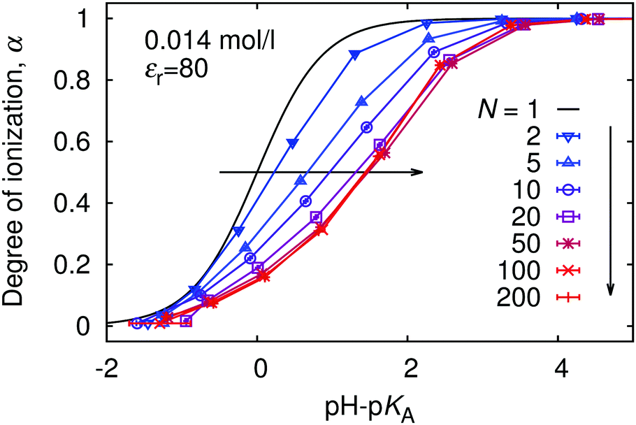
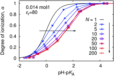
To investigate the role of further parameters influencing the ionization behaviour of weak PEs, we performed series of simulations with various chain lengths and polymer concentrations. We observed significant artifacts of periodic boundary conditions for N < 10 with single chain per simulation box. Therefore we fixed total number of monomer units per simulation box, such that nN = 100. For N ≥ 10 the difference between n = 10 and n = 1 was negligible at the given polymer concentration cpol = 0.014 M.
In Fig. 4 we show the titration curves for chain lengths 1 < N < 200. With N = 1 (single monomer) we match the ideal titration curve (eqn (6)). As we increase the chain length, the titration curves start to deviate from the ideal one, gradually moving to higher pH with respect to the ideal titration curve. Because the titration curves are not only shifted but also deformed with respect to the ideal one, it is clear that it is impossible to characterize the non-ideality of a polyelectrolyte chain by a single value of pKeff. Instead, pKeff becomes a parameter which depends on the degree of ionization of the chain, its length, concentration, etc. However, from N ≈ 50 the deviation from the ideal behaviour stays constant, nearly independent of the chain length. Therefore we claim that the shift and deformation of the titration curve is mostly a local effect of the nearest few monomer units along the chain contour. This observation is consistent with the earlier simulations of Ullner et al., who observed a very weak dependence (pKeff − pKA) ∼ α1/3(lnN)2/3 in the long chain limit.29 Fitting our data by eqn (11) with m as adjustable fit parameter we observe that this equation fairly well captures the shape of the deformed titration curves for various chain lengths (see ESI† Fig. S4). Interestingly, when we used eqn (9) with all its numerical pre-factors, the obtained value of m was very different from that from the fit, and the predicted curve was shifted to much higher values of pH, entirely outside the range of Fig. 4.
 |
| | Fig. 4 The titration curves for various lengths of polymer chains, N. | |
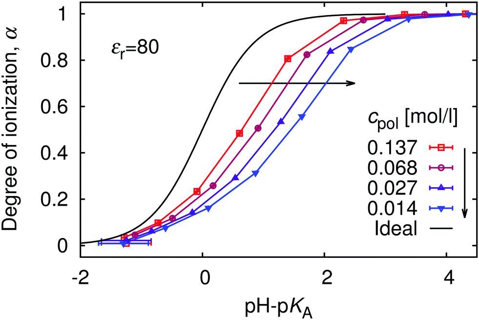
5.3 Influence of polymer concentration
The relation between the polymer concentration and the local concentration of H+ is further manifested in the concentration-dependence of the titration curves, shown in Fig. 5. We again observe the general trend that the titration curves are shifted to higher values of pH with respect to the ideal titration curve. The striking feature of this figure is that deviations from the ideal titration curve increase with dilution, quite opposite to the behaviour of simple acids, which become ideal when diluted. This observation is qualitatively consistent with increasing pKeff observed in the titration of both poly(acrylic acid) and poly(methacrylic acid).12,13 To understand this phenomenon we recall that the leading contribution to the deviation originates from electrostatic repulsion of nearby ionized groups. The counterions surrounding the chain screen this repulsion. However, with increasing polymer dilution the counterions are distributed over bigger volume, and their concentration near the chain drops (cf.Fig. 1), while the separation of ionized polymer segments remains practically the same. The lower concentration of counterions leads to weaker screening, and hence stronger repulsion of the bare charges on the chain. Ultimately, the stronger repulsion leads to suppressed ionization.
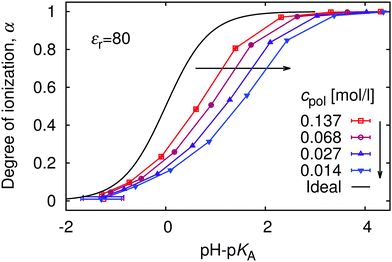 |
| | Fig. 5 The titration curves at various polymer concentrations, cpol. The black solid line is the ideal titration curve. | |
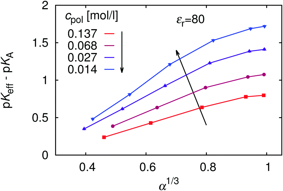
Since the deviation from ideal titration increases with dilution, it might provide an explanation why eqn (9) largely overestimates the shift: it has been derived neglecting the role of counterions, effectively assuming infinite dilution. To investigate this further, in Fig. 6 we re-plot the data from Fig. 5 in the form of the universal titration curve, eqn (11). In this representation we observe that only at low α the dependence is linear, in accordance with eqn (9) and (11), while above α ≈ 0.5 the simulation results deviate from the predicted linear dependence. In addition, the slope of the plots, which determines the parameter m, increases with dilution, so that at extreme dilution it might indeed reach the value predicted by eqn (9). The deviation from linearity beyond α = 0.5 could be attributed to the Manning condensation and strong correlations between the chain and its counterions. The Manning condensation is not captured by the theory of Katchalsky and Gillis and we will further address this point in the Section 5.4. We remark that for our system with flexible macromolecule of finite length and with inhomogeneous distribution of point charges the onset of Manning condensation is a gradual transition, as discussed by Mann et al.59 It can be identified from the plot of electrostatic energy per particle as a function of the Manning parameter (see ESI,† Fig. S5). In our case the plot features a broad flat maximum. For an infinitely long homogeneously charged rod the Manning condensation features a second order transition which can be identified by a cusp in the dependence of the electrostatic energy per particle on the Manning parameter.60,61
 |
| | Fig. 6 The universal titration curve compared with our simulation data for various polymer concentrations, cpol. | |
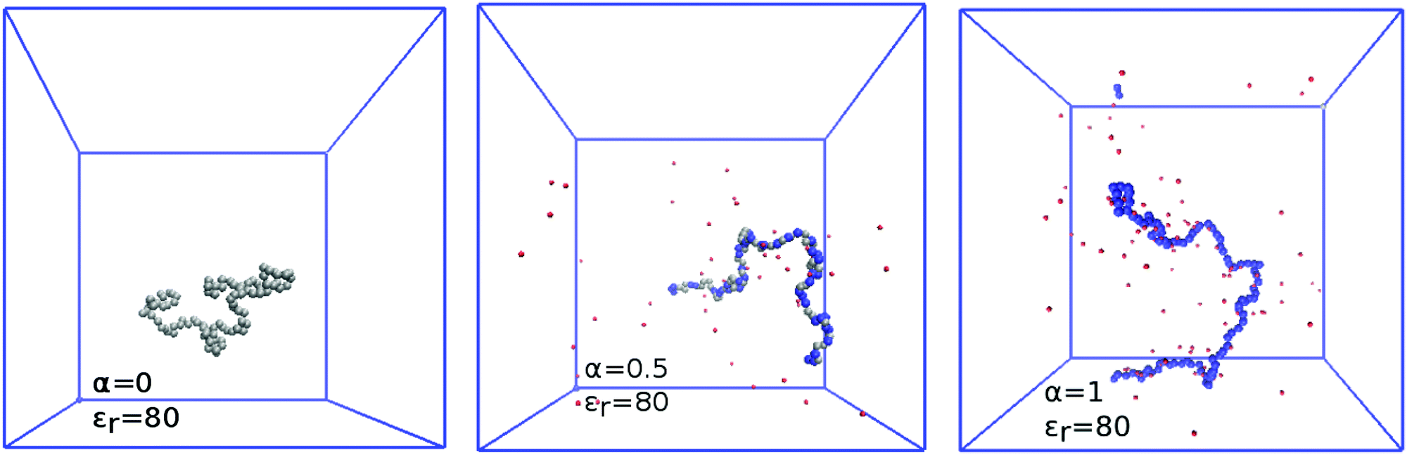
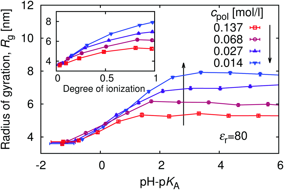
The complex shape of titration curves in Fig. 5 is a consequence of the interplay between the ionization of the polymer, and the accompanying conformational changes, illustrated by simulation snapshots in Fig. 7, and further by the dependence of the radius of gyration, Rg, on the degree of ionization in the insert of Fig. 8. Here we observe that the chain conformation changes from the swollen coil at α ≈ 0 to the nearly rod-like conformation at α ≈ 1. At the expense of entropy loss, the chain compensates in this way for the increased electrostatic repulsion at higher ionization. Furthermore, we observe in Fig. 8 that the maximum expansion of the chain increases with decreasing polymer concentration. Again, this can be understood when we recall from Fig. 1 that with decreasing cpol the concentration of H+ decreases in the whole range, so that the screening of charges on the chain vanishes. With weaker screening, the expansion due to electrostatic repulsion of the ionized groups is stronger. Fig. 8 also demonstrates that polymer segments are confined to a narrow region of the chain, while counterions are diluted: upon ten-fold decrease of concentration, the change of Rg at full ionization amounts to less than 50%. When Rg is plotted as a function of pH–pKA in Fig. 8, it appears to increase almost independently of cpol up to a certain value of pH where the expansion stops. This value depends on the polymer concentration, and from Fig. 5 we can see that it corresponds to the point where α approaches unity. Interestingly, comparison of Fig. 5 and 8 reveals that the nearly-matching values of Rg at the same pH but different polymer concentrations actually correspond to different degrees of ionization, α. The near coincidence of the Rg(pH–pKA) curves thus demonstrates an interesting cancellation of two non-ideal effects.
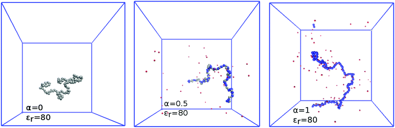 |
| | Fig. 7 Simulation snapshots showing polymer conformations at various degrees of ionization α. From left to right: α = 0, 0.5, and 1. Colour code: silver – uncharged monomer, blue – charged monomer, red – H+ ion. | |
 |
| | Fig. 8 Variation of the radius of gyration, Rg, with pH. | |
Last but not least, it is interesting to realize that as the polymer expands with increasing α, its overlap concentration, c* ∼ N/Rg3, decreases significantly (see ESI,† Fig. S6). Even if solution of the neutral polymer is prepared well below the overlap concentration, such that individual chains do not affect each other, as its conformation changes in the course of a titration experiment, the overlap concentration decreases and the fully ionized chains may significantly overlap and affect each other.
5.4 Influence of solvent permittivity
Replacing the solvent by another one with a different permittivity, or by continuous variation of composition of mixed solvents, it is possible to change the relative permittivity of the medium, and in this way to tune the electrostatic coupling strength u = lB/b. Within a narrower range, electrostatic coupling can also be varied by using a polymer with different separation of the charged groups.
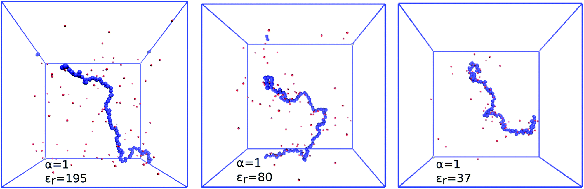
An increase in electrostatic coupling increases the enthalpy gain as the ions condense on the chain, while the corresponding entropy loss remains the same. This interplay of enthalpy and entropy has a non-trivial effect on the conformation, manifested in the non-monotonic dependence of Rg on u at fixed α in Fig. 9. At u ≲ 1 (high εr), typical for polar solvents, entropy dominates the behaviour of counterions. They are only weakly coupled to the chain, and contribute to the overall picture only through screening of the interactions between the charged monomers. At the same time, mutual repulsion between charges on the chain increases with u, therefore the chain expands and Rg(u) increases with u. Around the Manning condensation threshold, u ≈ 1, the ions start to condense, Rg(u) passes trough a maximum and starts to decrease again at higher u. At high coupling, the counterions become highly correlated with the chain. The alternating pattern of positive and negative charges along the chain brings about a net attractive force, termed the counterion-induced correlation attraction,62,63 which makes the polyelectrolyte shrink if u is further increased. This is well illustrated in Fig. 10 by simulation snapshots of the polymer with α = 1.0 at different electrostatic couplings: with increasing u an increasing portion of counterions is located in the immediate vicinity of the chain, and the chain extension decreases. The correlation effects require the discrete character of individual charged monomers and counterions to be explicitly considered, beyond the mean-field picture of the polyelectrolyte as a homogeneously charged worm-like chain in a cloud of counterions. For the same reason, if the electrostatic coupling is re-scaled by the degree of ionization as αu, the two curves of Rg(αu) in Fig. 9 for α = 0.3 and 1.0 do not collapse on a single universal master curve.
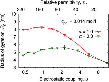 |
| | Fig. 9 Variation of the radius of gyration, Rg, with electrostatic coupling strength (bottom axis), and solvent permittivity, εr (top axis) at two degrees of ionization: α = 1.0 and α = 0.3 ± 0.08. See also ESI,† Fig. S8 for the complete data set of Rg(α, εr). | |
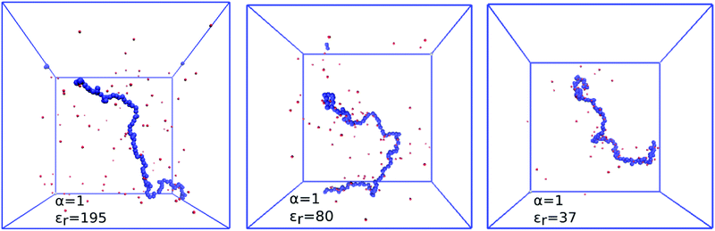 |
| | Fig. 10 Simulation snapshots showing counterion distribution and counterion condensation, from left to right: εr = 195, 80, 37, which correspond to u = 0.7, 1.7 and 3.8. Colour code: silver – uncharged monomer, blue – charged monomer, red – H+ ion. | |
The interplay between the chains and counterions at various permittivities can be also illustrated by distribution of counterions along the chain. Here we use the approach of Limbach et al.,58,64 who defined the distance of a given counterion from the chain as the smallest distance between that ion and any monomer unit. At long distances this function behaves indistinguishably from the conventional pair correlation function, g(r), up to r/Rcc ≈ 1/2, where it sharply drops to zero. At short distances, however, it respects the local symmetry of the problem: near the chain the distribution has local cylindrical symmetry while on long distances it is approximately spherical.
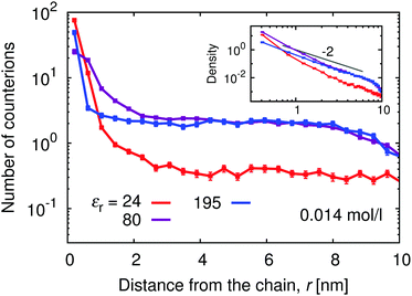
Above the counterion condensation threshold the condensed counterions compensate for the excess charge on the chain and effectively renormalize the coupling parameter to u ≈ 1. Therefore at α ≈ 1 the counterion condensation should not occur at εr ≳ 160, while at lower permittivities the number of condensed counterions should increase. We could estimate the number condensed counterions from the deviation of the plot in Fig. 11 in the vicinity of the chain from the plateau value at intermediate r. Note that this plateau only shows up at sufficiently low polymer concentrations (see ESI,† Fig. S7). At εr = 195 we observe that the curve is flat and only a few extra counterions are found in the immediate vicinity. With increasing coupling (decreasing εr) the positive deviation at low separations becomes more significant, as the counterions accumulate around the chain and fewer of them are found in the plateau region at higher separations.
 |
| | Fig. 11 Distribution of counterions along the polyelectrolyte chain for different relative permittivities, εr, at α = 1. | |
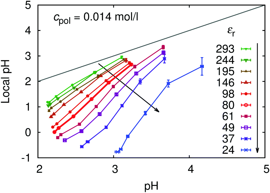
The counterion condensation has a profound influence on the local pH near the chain, as follows from Fig. 12. The slopes of the dependencies of local pH on pH in the bulk are much steeper at lower permittivities (stronger coupling), while at higher permittivities (weaker coupling) the local and bulk pH do not differ too much.
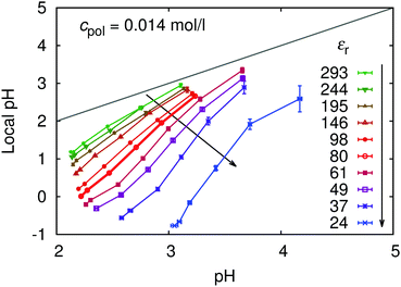 |
| | Fig. 12 Local pH in the vicinity of the chain, as a function of pH in the bulk for various solvent permittivities, εr. | |
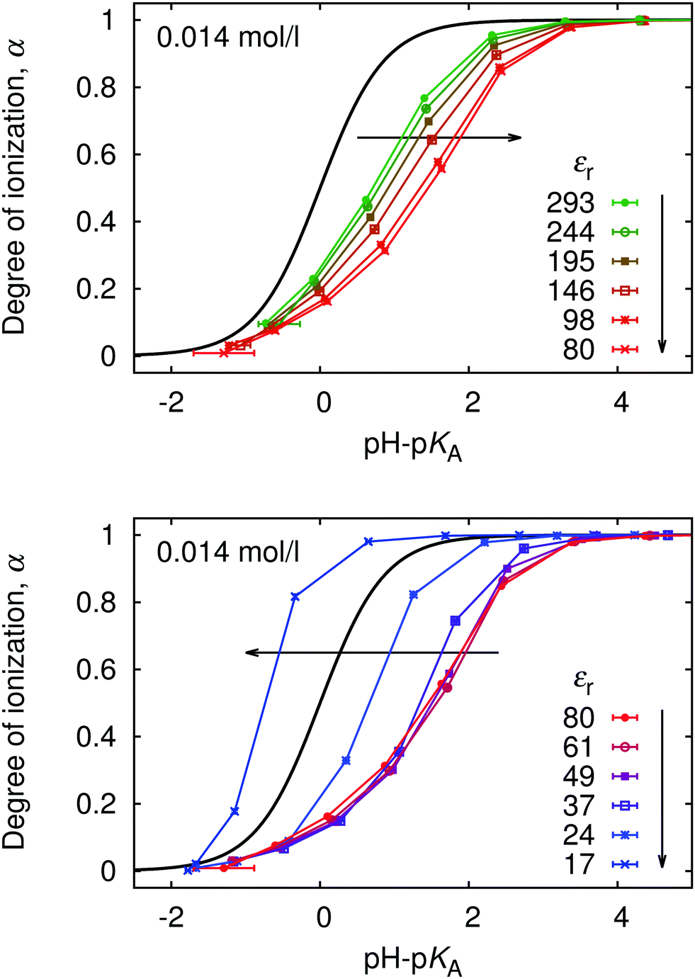
Since ionization behaviour of a weak polyelectrolyte is intimately coupled to its conformation, the profound differences in conformations and distribution of small ions which occur with varying permittivity, significantly affect the titration curves, as is shown in Fig. 13. As the electrostatic coupling increases up to u ≈ 2 (εr ≈ 80), the curves move towards higher values of pH–pKA and are increasingly deformed with respect to the ideal titration curve. At higher u the trend reverses, and the curves approach the ideal titration curve and even move to the opposite side of it at very low εr. This counter-intuitive phenomenon is not surprising when we consider the counterion-induced attraction at high u, which reduces the free energy cost of additional ionization. This observation is consistent with earlier work of Panagiotopoulos,32 who also observed that at very high u the polymer titration curve can be even shifted to the other side of the ideal one. It remains an open question, however, whether such total reversal of the behaviour could be observed in experiments. Real polymers exhibit specific polymer–counterion interactions, which are very difficult to properly include in the coarse-grained modeling. These specific interactions would presumably favor precipitation of he polymer from solution under such conditions.
 |
| | Fig. 13 The titration curves for various permittivities, εr. | |
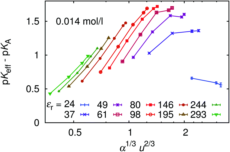
Finally, in Fig. 14 we plot our simulated titration curves at different εr as a function of α1/3u2/3. Following eqn (11) these data should collapse on a single straight line. At low u our data yield nearly straight lines but systematically shift to the right with increasing u (decreasing εr). At higher u our curves are increasingly deformed, which is presumably the consequence of counterion condensation. Thus we conclude that the universal master curve from eqn (9) and (11) does not provide an appropriate prediction of the dependence of α on εr even at low electrostatic coupling, while it completely fails at high coupling. However, if counterion condensation is not too strong, eqn (11) can still be used to fit experimental data and the above failure translates to the dependence of fit parameters pKA and m on εr.
 |
| | Fig. 14 The universal titration curve compared with our simulation data for different permittivities, εr. | |
6 Conclusion
In this work we have performed coarse-grained simulations of weak polyelectrolytes, explicitly accounting for the ionization equilibrium by means of the reaction ensemble method.50 This approach allowed us to explicitly consider the coupling between the ionization and conformation of a model polyelectrolyte chain. Using the simulation data, we have discussed the differences between the concentration of H+ ions in the bulk and in the immediate vicinity of the chain, commonly termed the “bulk pH” and the “local pH”. We have shown that the bulk and local pH can easily differ by two or more units, consistent with recent experimental observations.18,46 Next, we have investigated how the polymer chain length and concentration affect the titration curves. We observed that beyond N ≈ 20 the chain length effect is very weak which supports our claim that the non-ideal titration behaviour is mostly a local effect of the nearest groups on the chain. The decreasing polymer concentration results in an increasing non-ideality, opposite to the behaviour of simple acids which become ideal at infinite dilution. This counter-intuitive behaviour is consistent with experiments,12,13 and could be explained in terms of distribution of counterions and screening effects. Our investigation of the influence of electrostatic coupling strength (solvent permittivity) has revealed two regimes: at low coupling the non-ideality initially increases with decreasing εr as a consequence of increasing electrostatic repulsion. At high coupling the non-ideality decreases again and eventually changes the sign. At low coupling, the effect is dominated by increasing repulsion among the charged polymer segments, which is compensated at higher coupling by counterion condensation and effective attraction due to strong correlations between the chain and its ions. Finally, we have shown that simulation results at different permittivities exhibit systematic deviations from the expected universal master curve predicted by Katchalsky and Gillis, which is commonly used to fit experimental data.
Acknowledgements
We gratefully acknowledge Dr Oleg Rud for his discussions and comments to the manuscript. This research was supported by the Czech Science Foundation (grant P208/14-23288J) and the Ministry of Education, Youth and Sports (CUCAM CZ.02.1.01/0.0/0.0/15_003/0000417). Access to computing facilities of CERIT-SC (CZ.1.05/3.2.00/08.0144) and National Grid Infrastructure MetaCentrum (LM2010005) is acknowledged too.
References
- M. A. Dyakonova, N. Stavrouli, M. T. Popescu, K. Kyriakos, I. Grillo, M. Philipp, S. Jaksch, C. Tsitsilianis and C. M. Papadakis, Macromolecules, 2014, 47, 7561–7572 CrossRef CAS.
- M. A. Dyakonova, A. V. Berezkin, K. Kyriakos, S. Gkermpoura, M. T. Popescu, S. K. Filippov, P. Štépánek, Z. Di, C. Tsitsilianis and C. M. Papadakis, Macromolecules, 2015, 48, 8177–8189 CrossRef CAS.
- O. Colombani, E. Lejeune, C. Charbonneau, C. Chassenieux and T. Nicolai, J. Phys. Chem. B, 2012, 7560–7565 CrossRef CAS PubMed.
- O. Borisova, L. Billon, M. Zaremski, B. Grassl, Z. Bakaeva, A. Lapp, P. Stepanek and O. Borisov, Soft Matter, 2012, 8, 7649 RSC.
- O. V. Borisova, L. Billon, R. P. Richter, E. Reimhult and O. V. Borisov, Langmuir, 2015, 31, 7684–7694 CrossRef CAS PubMed.
- J. Xie, K. Nakai, S. Ohno, H.-J. Butt, K. Koynov and S. Yusa, Macromolecules, 2015, 48, 7237–7244 CrossRef CAS.
- K. Geisel, L. Isa and W. Richtering, Angew. Chem., Int. Ed., 2014, 53, 4905–4909 CrossRef CAS PubMed.
- A. J. Schmid, R. Schroeder, T. Eckert, A. Radulescu, A. Pich and W. Richtering, Colloid Polym. Sci., 2015, 293, 3305–3318 CAS.
- C. S. Patrickios and T. K. Georgiou, Curr. Opin. Colloid Interface Sci., 2003, 8, 76–85 CrossRef CAS.
- E. J. Kepola, E. Loizou, C. S. Patrickios, E. Leontidis, C. Voutouri, T. Stylianopoulos, R. Schweins, M. Gradzielski, C. Krumm, J. C. Tiller, M. Kushnir and C. Wesdemiotis, ACS Macro Lett., 2015, 4, 1163–1168 CrossRef CAS.
- T. Swift, L. Swanson, M. Geoghegan and S. Rimmer, Soft Matter, 2016, 12, 2542–2549 RSC.
- R. Arnold, J. Colloid Sci., 1957, 12, 549–556 CrossRef CAS.
- C. Heitz, M. Rawiso and J. François, Polymer, 1999, 40, 1637–1650 CrossRef CAS.
- A. Katchalsky and J. Gillis, Recl. Trav. Chim. Pays-Bas, 1949, 68, 879 CrossRef CAS.
- F. Plamper, H. Becker, M. Lanzendorfer, M. Patel, A. Wittemann, M. Ballauff and A. Müller, Macromol. Chem. Phys., 2005, 206, 1813–1825 CrossRef CAS.
- G. Xu, S. Luo, Q. Yang, J. Yang and J. Zhao, J. Chem. Phys., 2016, 145, 144903 CrossRef PubMed.
- S. Wang, S. Granick and J. Zhao, J. Chem. Phys., 2008, 129, 241102 CrossRef PubMed.
- C. Qu, Y. Shi, B. Jing, H. Gao and Y. Zhu, ACS Macro Lett., 2016, 402–406 CrossRef CAS.
-
S. P. L. Sörensen, Carlsberg Laboratorien, Kopenhagen, 1909, vol. II, pp. 131–200 Search PubMed.
-
I. N. Levine, Physical Chemistry, Mc Graw Hill, VI edn, 2009 Search PubMed.
- R. P. Buck, S. Rondinini, A. K. Covington, F. G. K. Baucke, C. M. A. Brett, M. F. Camoes, M. J. T. Milton, R. Mussini, R. Naumann, K. W. Pratt, P. Spitzer and G. S. Wilson, Pure Appl. Chem., 2002, 74, 2169 CrossRef CAS.
- H. J. Limbach, C. Holm and K. Kremer, Europhys. Lett., 2002, 60, 566–572 CrossRef CAS.
- P. Košovan, Z. Limpouchová and K. Procházka, Macromolecules, 2006, 39, 3458–3465 CrossRef.
- E. Raphael and J. F. Joanny, Europhys. Lett., 1990, 13, 623 CrossRef CAS.
- F. Uhlík, P. Košovan, Z. Limpouchová, K. Procházka, O. V. Borisov and F. A. M. Leermakers, Macromolecules, 2014, 47, 4004–4016 CrossRef.
- J. L. Lützenkirchen, J. V. Male, F. Leermakers and S. Sjöberg, J. Chem. Eng. Data, 2011, 1602–1612 CrossRef.
- M. Borkovec, G. J. Koper and C. Piguet, Curr. Opin. Colloid Interface Sci., 2006, 11, 280–289 CrossRef CAS.
- M. Lund and B. Jönsson, Q. Rev. Biophys., 2013, 46, 265–281 CrossRef CAS PubMed.
- M. Ullner, B. Jönsson and P. Widmark, J. Chem. Phys., 1994, 100, 3365 CrossRef CAS.
- M. Ullner and C. E. Woodward, Macromolecules, 2000, 33, 7144–7156 CrossRef CAS.
- B. Jönsson, M. Ullner, C. Peterson, O. Sommelius and B. Södeberg, J. Phys. Chem., 1996, 100, 409–417 CrossRef.
- A. Panagiotopoulos, J. Phys.: Condens. Matter, 2009, 21, 424113 CrossRef CAS PubMed.
- S. Uyaver and C. Seidel, Europhys. Lett., 2003, 64, 536–542 CrossRef CAS.
- S. Uyaver and C. Seidel, Macromolecules, 2009, 42, 1352–1361 CrossRef CAS.
- T. Zito and C. Seidel, Eur. Phys. J. E: Soft Matter Biol. Phys., 2002, 8, 339–346 CrossRef CAS PubMed.
- M. Ullner, B. Jönsson, B. Söderberg and C. Peterson, J. Chem. Phys., 1996, 104, 3048–3057 CrossRef CAS.
- M. Ullner and B. Jönsson, Macromolecules, 1996, 29, 6645–6655 CrossRef CAS.
- S. Ulrich, A. Laguecir and S. Stoll, J. Chem. Phys., 2005, 122, 094911 CrossRef PubMed.
- F. Carnal, S. Ulrich and S. Stoll, Macromolecules, 2010, 43, 2544–2553 CrossRef CAS.
- S. Edgecombe, S. Schneider and P. Linse, Macromolecules, 2004, 37, 10089–10100 CrossRef CAS.
- G. S. Longo, M. O. de la Cruz and I. Szleifer, Macromolecules, 2011, 44, 147–158 CrossRef CAS.
- G. S. Longo, M. O. de la Cruz and I. Szleifer, ACS Nano, 2013, 7, 2693–2704 CrossRef CAS PubMed.
- J. Ziebarth and Y. Wang, J. Phys. Chem. B, 2010, 114, 6225–6232 CrossRef CAS PubMed.
- J. D. Ziebarth and Y. Wang, Biomacromolecules, 2010, 11, 29–38 CrossRef CAS PubMed.
- S. Luo, X. Jiang, L. Zou, F. Wang, J. Yang, Y. Chen and J. Zhao, Macromolecules, 2013, 46, 3132–3136 CrossRef CAS.
- S. Wang and Y. Zhu, Soft Matter, 2011, 7, 7410–7415 RSC.
- F. Uhlík, P. Košovan, E. B. Zhulina and O. V. Borisov, Soft Matter, 2016, 12, 4846–4852 RSC.
- M. Vögele, C. Holm and J. Smiatek, J. Chem. Phys., 2015, 143, 243151 CrossRef PubMed.
-
R. A. Butler, PhD thesis, University of Florida, 1978.
- W. R. Smith and B. Tříska, J. Chem. Phys., 1994, 100, 3019–3027 CrossRef CAS.
- S. Duane, A. Kennedy, B. J. Pendleton and D. Roweth, Phys. Lett. B, 1987, 195, 216–222 CrossRef CAS.
- A. Irbäck, J. Chem. Phys., 1994, 101, 1661–1667 CrossRef.
- U. Wolff, Comput. Phys. Commun., 2004, 156, 143–153 CrossRef CAS.
-
O. V. Borisov, E. B. Zhulina, F. A. Leermakers, M. Ballauff and A. H. E. Müller, in Self Organized Nanostructures of Amphiphilic Block Copolymers I, ed. A. H. E. Müller and O. Borisov, Springer Berlin Heidelberg, 2011, vol. 241, pp. 1–55 Search PubMed.
-
D. A. McQuarrie, Statistical Mechanics, Harper Collins, New York, 1976 Search PubMed.
- V. Ballenegger, A. Arnold and J. J. Cerdà, J. Chem. Phys., 2009, 131, 094107 CrossRef CAS PubMed.
- J. S. Hub, B. L. de Groot, H. Grubmüller and G. Groenhof, J. Chem. Theory Comput., 2014, 10, 381–390 CrossRef CAS PubMed.
- H. J. Limbach and C. Holm, J. Chem. Phys., 2001, 114, 9674–9682 CrossRef CAS.
- B. A. Mann, C. Holm and K. Kremer, Macromol. Symp., 2006, 237, 90–107 CrossRef CAS.
- A. Naji and R. R. Netz, Phys. Rev. Lett., 2005, 95, 185703 CrossRef PubMed.
- A. Naji and R. R. Netz, Phys. Rev. E: Stat., Nonlinear, Soft Matter Phys., 2006, 73, 056105 CrossRef PubMed.
- Q. Liao, A. V. Dobrynin and M. Rubinstein, Macromolecules, 2006, 39, 1920–1938 CrossRef CAS.
- A. Naji, S. Jungblut, A. G. Moreira and R. R. Netz, Phys. A, 2005, 352, 131–170 CrossRef.
- H. J. Limbach and C. Holm, J. Phys. Chem. B, 2003, 107, 8041–8055 CrossRef CAS.
Footnote |
| † Electronic supplementary information (ESI) available. See DOI: 10.1039/c7cp00265c |
|
| This journal is © the Owner Societies 2017 |
Click here to see how this site uses Cookies. View our privacy policy here. 
 Open Access Article
 This Open Access Article is licensed under a Creative Commons Attribution-Non Commercial 3.0 Unported Licence
 *
*

 is the standard Gibbs free energy change of the reaction, νi is the stoichiometric coefficient and μi the chemical potential of species i participating in the reaction. The chemical potential can be further written in terms of activity
 , and νi is the stoichiometric coefficient of species i in the reaction eqn (1) (negative for the reactants and positive for the products). The instantaneous number of species i in the simulation box, Ni is linked to its the initial number, N0i through the extent of reaction, ξ: