Mechanism and kinetics of the electrocatalytic reaction responsible for the high cost of hydrogen fuel cells

Abstract

The sluggish oxygen reduction reaction (ORR) is a major impediment to the economic use of hydrogen fuel cells in transportation. In this work, we report the full ORR reaction mechanism for Pt(111) based on Quantum Mechanics (QM) based Reactive metadynamics (RμD) simulations including explicit water to obtain free energy reaction barriers at 298 K. The lowest energy pathway for 4 e⁻ water formation is: first, *OOH formation; second, *OOH reduction to H₂O and O*; third, O* hydrolysis using surface water to produce two *OH and finally *OH hydration to water. Water formation is the rate-determining step (RDS) for potentials above 0.87 Volt, the normal operating range. Considering the Eley–Rideal (ER) mechanism involving protons from the solvent, we predict the free energy reaction barrier at 298 K for water formation to be 0.25 eV for an external potential below U = 0.87 V and 0.41 eV at U = 1.23 V, in good agreement with experimental values of 0.22 eV and 0.44 eV, respectively. With the mechanism now fully understood, we can use this now validated methodology to examine the changes upon alloying and surface modifications to increase the rate by reducing the barrier for water formation.

---

Polymer-electrolyte (or proton-exchange) membrane (PEM) fuel cells utilizing hydrogen (H₂) and oxygen (O₂) to produce electricity^1–4 promise environmentally sustainable energy technology to replace traditional fossil fuel technology. Although prototype automobiles powered by hydrogen fuel cells are being demonstrated, dramatic improvements are essential for large-scale, cost-effective commercialization.⁵ The challenges and opportunities are well summarized in review papers.^6–8

The slow electrocatalysis of the oxygen reduction reaction (ORR) looms as the central issue. Currently, the best ORR catalysts are based on Pt or Pt alloys, but after years of research, the performance remains inadequate, requiring far too much Pt to be economical and requiring a considerable overpotential, η ∼0.3 V.^9–12 For example, the DOE targets are A_s = 0.7 mA cm⁻² (2015) and A_m = 0.44 A per mg_pt (2017)⁵ whereas the best commercial Pt/C catalysts have a specific activity A_s = 0.127 mA cm⁻² and a mass activity A_m = 0.096 A per mg_pt at 0.9 V under working conditions.¹³

Catalysis performance has been improved significantly by nanoscale designs including alloying of Pt with such metals as Ni or Co.¹⁴ Other promising reports^15–19 include a Mo–Pt₃Ni/C catalyst claimed to exceed DOE targets.¹³ However, many suggested systems have problems with performance degradation (e.g., dealloying).^4,20

We consider that catalyst development is hampered by an incomplete understanding of the reaction mechanism underlying the ORR. Several general guidelines based on theoretical insights and experimental observations have been proposed,²¹ but there is no consensus of the controlling factors underlying ORR.

The ORR reaction involves three basic steps:^22,23

(1) Breaking the O–O bond, which may be

(a) Dissociative

*O₂ → O* + O* (1a)

(b) Associatively dissociative (Jacob and Goddard²⁴)

*O₂ + H⁺ + e⁻ → *OOH (1b)

*OOH → *OH + O* (1c)

(c) Associatively reductive (a new mechanism we report here)

*O₂ + H⁺ + e⁻ → *OOH (1b)

*OOH + H⁺ + e⁻ → H₂O(aq) + O* (1c′)

(2) Conversion of O* to *OH, which may occur by

(a) Electrochemical reduction

O* + H⁺ + e⁻ → *OH (2a)

(b) Langmuir–Hinshelwood (LH) hydrolysis using surface H₂O* (Sha, Goddard, and coworkers²⁵)

O* + H₂O* → *OH + *OH (2b)

(3) Conversion of OH* to H₂O

*OH + H⁺ + e⁻ → H₂O (3)

These various reaction mechanisms lead to several possible rate-determining steps (RDS).

In the work of Gómez-Marín and Feliu,²⁶ kinetic analysis of the cyclic voltammetry profile showed that the cathodic current depends to first-order on the O₂ concentration in agreement with rotating disk electrode (RDE) experiments.²⁷ The linearity of the Koutecky–Levich plot was considered as evidence that the RDS is the first electron transfer step. Therefore, either *O₂⁻ formation in base solution²⁸ or hydroperoxyl (*OOH) formation (1b) in acid solution was proposed to be the RDS.^29–31 However, recent kinetics simulations show that this first order O₂ dependency can be explained by slow adsorption of O₂ into the solution, leading to a low O₂ concentration and slow solvent reorganization at the interface.³² Therefore, the first electron transfer step need not be the RDS, even though the overall reaction rate is of order one in O₂. This opens up the possibilities of other elementary reaction steps as the RDS.

For example, the water formation step (3) has also been widely proposed as the RDS based on experiments showing significant hydroxyl concentration (*OH) under working conditions,³³ indicating that either the *OH species is an ORR intermediate or the reactant.^34–36 This was supported by QM calculations showing that adsorbed oxygen and *OH are stable intermediates at potentials close to equilibrium.²¹ Furthermore, DFT calculations with explicit consideration of the reconstructed surface indicated that *OH removal from the surface determines the overpotential.³⁷

Nevertheless, reaction kinetics under real operating conditions may be much more complex. Very possibly, ORR kinetics is not determined solely by a single factor, but with multiple RDS coexisting. Indeed, a recent experiment demonstrated that under operating conditions two phases of *OH coexist: hydrated *OH and non-hydrated *OH. Moreover, the possible coexistence of two sets of kinetics has been demonstrated by DFT calculations: H₂O formation could be the RDS in the hydrated pathway, while *OOH formation is the RDS in the non-hydrated pathway.³⁸

Other possible ORR reaction mechanisms have been discussed in previous studies.^25,26 Such controversies in the ORR reaction mechanism could be resolved by determining the reaction intermediates experimentally. However, in situ experimental methods have not been able to detect oxygenated adsorbed species reliably. Nano-electronic strategies are in development for in situ electrochemical surface studies with high surface sensitivity and surface specificity, which might eventually extend the understanding of the nature of catalysis interface and ORR reaction mechanism.³⁹

Quantum mechanics (QM) calculations can provide critical atomistic mechanistic insight about ORR reactions. However, previous studies have all been deficient in including the effect of the solvent fully. Early calculations ignored the solvent, while later ones used implicit solvation methods sometimes with a few explicit solvent molecules.^7,24,25,40 Explicit simulation of solvent^41–44 becomes more popular attribute to the upgrade in hardware and software. These various solvation models have led to a range of inconsistent results. For example, the predicted free energy barriers for O₂ dissociation range from 0.0 eV to 0.7 eV, depending on the solvation model.^23,25,40 Consequently, we concluded that it is essential to use ∼5 layers of explicit waters to describe reactions at the catalyst–solvent interface properly. Indeed, because the extrapolated experimental apparent activation energy at 0.8 V is only 0.2 eV to 0.6 eV,^45–48 the QM barriers must be accurate to 0.1 to 0.2 eV to pinpoint the key steps.

Here we simulate the water/Pt(111) interface using 48 explicit water molecules on a 4 × 4 × 3 Pt(111) surface slab with area 1.08 nm². This leads to 5 layers of explicit water with a thickness of 1.5 nm, as shown in Fig. 1A. To equilibrate the waters interacting with the interface, we need to carry out ∼2 ns of molecular dynamics at 298 K NVT, but Reactive Molecular Dynamics (RMD) using Quantum Mechanics (QM) forces (termed AIMD) is practical on this system for only 10 ps or so. Thus to fully equilibrate the water–Pt interface, we carried out 2 ns of RMD simulations using the ReaxFF reactive force field⁴⁹ for Pt and H₂O. Starting from this well-equilibrated interface, we made 10 ps of AIMD simulation at 298 K using metadynamics to calculate the free energy barriers for each of numerous possible reaction steps. We consider that this model of QM with explicit treatment of the water dynamics at operating temperature provides a reliable description of the reaction kinetics.

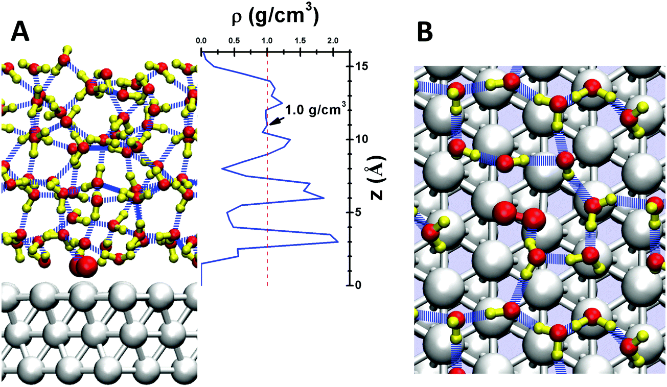Fig. 1 (A) Side view showing a snapshot at 298 K of the surface structure of the water/Pt(111) interface, with 5 layers of solvent (48 H₂O molecules plus one O₂), (B) top view of the first contact layer, leading to 11 water in the surface layer plus one O₂ bonded to Pt surface for a total coverage of 3/4 ML. (Note that the 3rd layer Pt are not shown in B.) The water density distribution (center of mass) perpendicular to the surface (z direction) is shown between (A) and (B), where the reference 0 is at the centers of the surface Pt atoms. The red slashed line indicates the density of bulk water at 298 K (1.0 g cm⁻³). The Hydrogen bond (HB) networks are shown in blue dashed lines. The colors of atoms are Pt in silver, H in yellow and O in red.

Fig. 1A shows the density profile of the water layers, with three clear peaks near the surface. The first peak at ∼3 Å from the Pt surface corresponds to the first contact layer of water, consisting of 11 water molecules with one chemisorbed O₂ leading to a surface coverage close to the 2/3 ML suggested by the bilayer water model.⁵⁰ This first contact layer of water contains an integrated hydrogen bond network (shown in Fig. 1B), but with irregular and fluctuating five member rings and six member rings rather than the perfect six member rings from energy minimized structures.⁵¹ The presence of O₂ in this first layer slightly distorts the hydrogen bond (HB) network, so that this O₂ forms one HB with a water molecule in the second layer. The density of the first layer is about 2.0 g cm⁻³, twice that of bulk water. The second layer leads to a significant peak between 0.6 and 0.7 nm, slightly longer than the normal 0.3 nm HB distance away from the first layer. The third layer is less structured but distinguishable; the protonated water prefers this layer. These three layers have a total thickness of ∼1 nm, providing the most relevant regions for surface reactions. For the next ∼0.2 nm (1.0 nm to 1.2 nm) the density is ∼1.0 g cm⁻³, the bulk value of water at 298 K. Finally, at 1.5 nm we reach the vapor/liquid interface which is ∼0.2 nm thick. No evaporated water was observed in the RMD simulations. These results demonstrate that a 1.5 nm thick water layer is sufficient to simulate the interface reactions (Table 1).

Table 1 The free energy barriers (ΔG^‡_AIMD, in eV) derived from QM reactive metadynamics (RμD simulations and the free energy barriers after correcting for the change in potential to the saddle point (ΔG^‡, in eV). The standard deviations estimated from three independent simulations are shown in parenthesis. The potentials in the simulations for ER mechanism were controlled by adding one H₃O (H₃O + e⁻) for 0.6 V case and by adding one H₃O + Cl (H₃O⁺ + Cl⁻) for 1.1 V case. In such QM calculations, the number of electrons is constant so that the potentials changes along with the reactions. For the cases of ER reaction, this requires corrections to determine the free energy barrier at a constant potential. Details are in Section S5 of the ESI

Step	Reactions	Reaction equations	ΔG^‡AIMD (eV)	ΔG^‡ (eV)
1a	*O2 dissociation	*O2 → O* + O*	0.40 (3)
1b	*O2 association (LH)	*O2 + H* → *OOH	0.22 (7)
1c	*OOH dissociation	*OOH → O* + OH*	0.38 (8)
1c′	*OOH reduction (LH)	*OOH + H* → H2O + O*	0.29 (7)
1c′	*OOH reduction (ER@0.6V)	*OOH + H^+ + e^− → H2O + O*	0.14 (6)
1c′′	HOOH formation (LH)	*OOH + H* → HOOH	0.48 (5)
2c	O* hydrolysis (LH)	O* + H2O* → *OH + *OH	0.25 (6)
3a	Water formation (LH)	*OH + H* → H2O	0.54 (8)
3b	Water formation (ER@0.6 V)	*OH + H^+ + e^− → H2O	0.16 (7)	0.12 (13)
3b	Water formation (ER@1.1 V)	*OH + H^+ + e^− → H2O	0.39 (6)	0.35 (12)

---

This pure water/Pt interface corresponds to the catalysis surface in the diffusion region of the ORR reactions (0.3 V to 0.6 V). For more positive potentials, *OH may accumulate on the surface, so that under working condition (0.8 V to 0.9 V) the surface layer may be partially dissociated, including both water and hydroxyl (*OH). However, kinetic analyses conclude that dissociated surface H₂O has only a slight negative electronic effect on ORR kinetics for the case of a weak acid compared with the pure water/Pt surface.³² This suggests that the reaction mechanisms are similar even if the surface has dissociated water. Therefore, the ORR reaction mechanism derived here based on the water/Pt surface should also apply to the real surface at 0.8 to 0.9 V.

We carried out metadynamics QM simulations at 298 K to predict the reaction free energy barriers for all plausible ORR elementary steps in reactions (1), (2), and (3). The Langmuir–Hinshelwood (LH) model has been used in previous calculations that did not contain an explicit solvent to simulate the electrochemical reaction, in which case H* is related to H⁺ + e⁻ by H⁺ + e⁻ → H*.^7,20

Results and discussion

O–O decomposition

Starting with O₂ at the bridge site, we applied meta-forces continuously to accumulate the population along the O–O (r_O–O) collective variable (CV) distance, driving the O₂ to dissociate. Snapshots from the reactive trajectories are shown in Fig. 2. Surprisingly, as the O₂ dissociates to form two O*, we observe that one O* at the on-top site is immediately hydrolyzed by a surface water through a Grotthuss mechanism involving a second aqueous water molecule (reaction trajectories in Fig. S1, ESI†). Therefore, instead of decomposing into two O* as indicated in (1a) we observed the overall reaction as follows,This O* hydrolysis reaction (2c) is similar to that discovered by Sha, Goddard, and coworkers,²⁵ except now we find a 2nd (aqueous) water also to be involved.

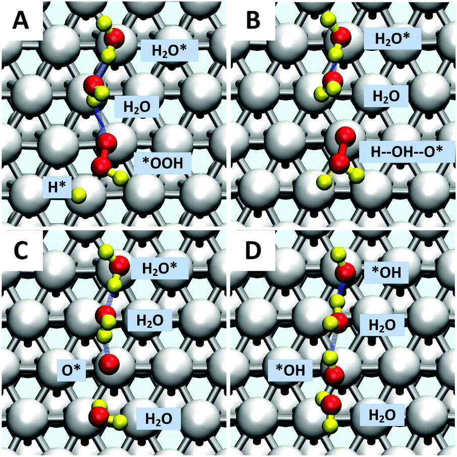Fig. 2 Reactive trajectories from meta-dynamics showing the *OOH reduction (1c′) along with oxygen hydrolysis (2c). . (A) t = 0 ps. *OOH with the terminal O bonded on the top site, and the H* making an HB to the middle O. (B) t = 0.38 ps. H* attacks the O(H) of *OOH to form an H⋯*OOH complex. (C) t = 0.42 ps. The reaction started in step b has completed with a surface H₂O* plus O* on the top site (reaction (1c′)). The free energy barrier for this process is ΔG^‡ = 0.29 eV (D) t = 0.51 ps. O* undergoes hydrolysis via a surface water via a Grotthuss process, through an intermediate water molecule leaving two *OH on the surface (reaction (2c)). The free energy barrier for this process at 298 K is 0.25 eV. The colors of atoms are Pt in silver, H in yellow (for viewing convenience), and O in red.

*OOH formation

Jacob and Goddard²⁴ suggested an alternative direct decomposition: instead, O₂ can react with H* to form *OOH (associative step (1b)), followed by a subsequent dissociation step (1c). We calculate ΔG^‡ = 0.22 eV for *OOH formation (as shown in Fig. S3, ESI†), significantly lower than for direct O–O dissociation. However, with explicit solvent, we find that the direct *OOH dissociation (1c) into O* and *OH has ΔG^‡ = 0.38 eV. To establish this, we considered a two-dimensional CV that includes both the O–O distance and dihedral angle of Pt–O–O–H. This shows that the association and decomposition are decoupled, as shown in the ESI† (Fig. S4).

*OOH reductive decomposition

Instead of (1c), we find that *OOH undergoes reductive decomposition (1c′) using a surface H₂O to form H₂O* + O* with ΔG^‡ = 0.15 eV, making (1c′) much more favorable than (1c). Surprisingly, we observe that the product O* is immediately hydrolyzed by a surface H₂O (reaction (2c)) as shown in Fig. 2C and D, a reaction similar to that found for *O₂ decomposition. Therefore, the overall reaction for O–O dissociation mechanism (1b−2c) is (as shown in Fig. 2):Therefore, the indirect HOO* association pathway (ΔG^‡ = 0.22 eV) followed by *OOH reductive decomposition (ΔG^‡ = 0.29 eV) is much more favorable for breaking the O₂ bond than direct dissociation (ΔG^‡ = 0.40 eV) or HOOH* decomposition (0.38 eV).

This high reactivity of surface water, H₂O*, has not previously been suggested (we discovered it first in unpublished ReaxFF reaction simulations). The reason why surface H₂O is so reactive is that the binding energy of H₂O to Pt is only 0.2 eV insolvent, while *OH binds by 1.0 eV (referenced to H₂ + H₂O), making the OH bond of surface water 0.8 eV more active than normal H₂O.

The second hydrolysis step was observed during the timescale of the O₂ dissociation step, suggesting that some of the reaction energy of the 1st step may help drive this second step, rather than being dissipated. The small O* hydrolysis barrier of 0.25 eV (Fig. S2, ESI†) indicates that surface water may play a major role in ORR reactions and it shows that non-electrochemical steps may accelerate an overall electrochemical reaction, providing a potentially useful design principle for electrocatalytic processes.

The presence of *OOH also leads to the possibility of HOOH formation (1c′′), but we find ΔG^‡ = 0.48 eV, which is the largest barrier among the three branches from *OOH. This indicates that HOOH formation is unfavorable on Pt(111), consistent with the lack of HOOH formation observed experimentally for Pt(111) under ORR conditions.⁵²

Water formation

The final reaction step is water formation

*OH + H⁺ + e⁻ → H₂O(aq) (3a)

Here we find that ΔG^‡ = 0.54 eV, with reactive snapshots as shown in ESI† (Fig. S5).

Summarizing, the free energy barriers for the various reduction steps are:

(1) ΔG^‡ = 0.22 eV for O₂ association (1b);

(2) ΔG^‡ = 0.29 eV for *OOH reduction (1c′) and 0.25 eV for O* hydration by surface water (2b);

(3) ΔG^‡ = 0.54 eV for water formation (3a).

Therefore, the reaction mechanism describing the minimal energy kinetic pathway is as follows:

With a rate-determining step (RDS) of ΔG^‡ = 0.54 eV.

These free energy barriers were identified with normal finite temperature QM RMD in which the number of electrons is fixed. To convert these values to constant applied potential conditions of the experiments, we used the post-QM correction method proposed by Chan and Nørskov,⁵³ but we replace the charge (which is ambiguous in plane wave DFT calculations) with capacitance. Details for calculating these corrections to the various reaction steps are tabulated in the ESI† (Table S1).

Reaction via ER

For potentials U > 0.3 V, the LH model used above fails to match the experiment conditions since it is energetically more favorable for H* to detach to form H₃O⁺ + e⁻. Therefore, the reaction kinetics predicted from LH model cannot be compared directly with experimental data. Instead, for U > 0.3 V we consider the Eley–Rideal (ER) model, in which H₃O⁺ + e⁻ is the reactant, to describe the reduction reactions involving hydrogen.

For QM RMD simulations of reactions involving H₃O⁺ + e⁻, we replace one of the 48 H₂O with H₃O, which becomes H₃O⁺ with an increased electron density on the Pt electrode. The extra electron increases the Pt work function (WF) leading to U = 0.6 V. Because the number of electrons is constant as the reaction path is sampled in metadynamics, the WF changes along the reaction coordinate. These potential changes can influence the rate of water formation since water formation is thermodynamically favorable at 0.6 V, but unfavorable at 1.0 V. Therefore, we used collective variables that constrain both of the two OH bond lengths to force water formation. The calculated free energies were corrected back to 0.6 V based on the calculated changes going through the transition state.

The inclusion of Pt–O in the CV makes it necessary to ensure that the water product detaches from the surface site. The two-dimensional free energy surface calculated with this CV is shown in Fig. 3A. At 0.6 V, the free energy barrier from the QM RMD is 0.16 eV, which becomes 0.12 eV after correction for constant potential. The reaction pathway for proton transfer is shown in Fig. 4. In these simulations, we found that the proton forms an H₅O₂⁺ complex involving one water molecule from the first layer and a 2nd water molecule from the 2nd layer. Three intermediate water molecules participate in bridging H₅O₂⁺ and *OH via a Grotthuss HB proton tunneling network as shown in Fig. 4.

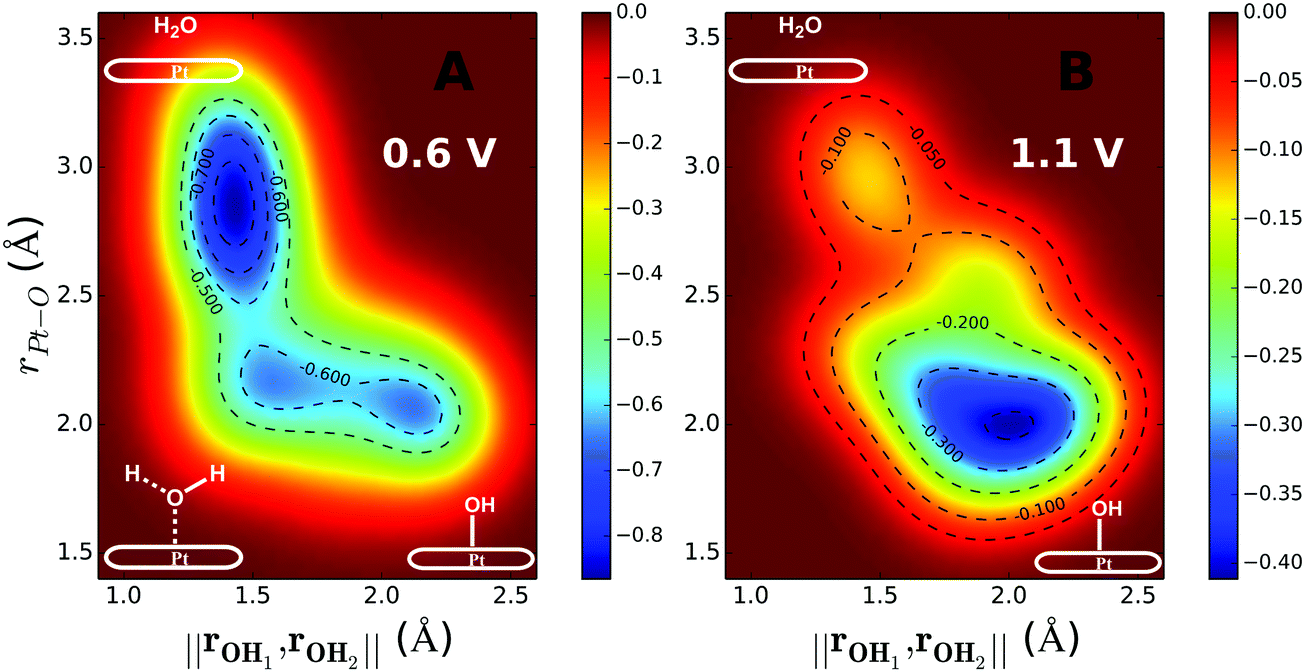Fig. 3 Two-dimensional free energy contours for water formation through the ER mechanism at 0.6 V potential (A) and 1.1 V potential (B). The free energy barrier for water formation (H₃O⁺ + e⁻ + *OH → H₂O + H₂O) derived from the QM RμD simulation is ΔG^‡ = 0.16 eV for 0.6 V and ΔG^‡ = 0.39 eV for 1.1 V. After correcting for the change in the potential along the reaction path (the potential goes up when the e⁻ is used to form water) to obtain the barrier for constant potential we obtain ΔG^‡ = 0.12 eV for U = 0.6 V and 0.35 eV for U = 1.1 V. The potentials were controlled by adding one H₃O (H₃O⁺ + e⁻) for the case of 0.6 V and adding one H₃O and one Cl (H₃O⁺ + Cl⁻) for the case of 1.1 V. The two collective variables are: (1) norm of r_OHa and r_OHb, (, where, H_a is the hydrogen in OH*, and H_b is the nearest hydrogen from the nearby H₂O.) It is necessary to constrain two OH distances to ensure that the final product is water (H_a–O–H_b). When water forms, ‖r_OHa, r_OHb‖ is about 1.41 Å. (2) The distance between O (OH*) and Pt (r_Pt–O).

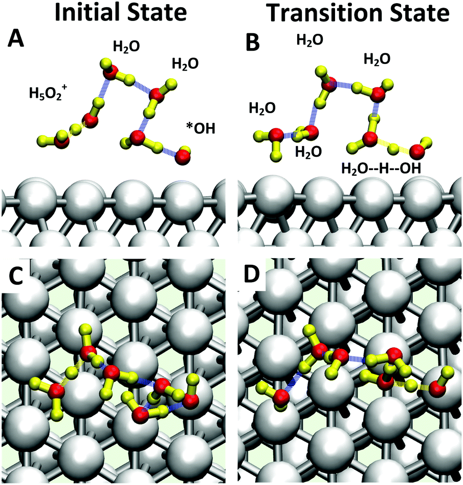Fig. 4 Snapshots of structures formed during the ER mechanism for water formation (3b). H₃O⁺ + e⁻ + *OH → H₂O + H₂O) from the QM RμD reaction trajectory at 0.6 V potential with one extra H₃O (H₃O⁺ + e⁻) initial state (A). Top view and (C) side view and transition state (B). Top view and (D) side view. The reaction starts with one H₅O₂⁺ complex and one *OH. Three intermediate water molecules are involved in proton tunneling, a Grotthuss mechanism. The colors of atoms are Pt in silver, H in yellow, and O in white. Water molecules not involved were hidden, for viewing convenience.

The reaction barriers for constant potential conditions depend on the magnitude of the potential. Experimentally, this dependence can be characterized by the symmetry factor (β), which is related to the fraction of the charge transfer that occurs in the transition state. Experimentally, β is derived from the Tafel slope by applying a series of potentials. In our simulations, we control the potential by adding ions into the system. For example, introducing one Cl into the system increases the potential from 0.6 to 1.1 V, because Cl extracts an e⁻ from the electrode to form Cl⁻, thereby increasing the WF to a more positive potential. The two-dimensional free energy surface for water formation (ER) calculated at 1.1 V is shown in Fig. 3B. At this voltage, water formation is already energetically unfavorable. Therefore, the free energy is uphill from *OH to water. The free energy barrier predicted from the metadynamics is 0.39 eV, which becomes is 0.35 eV after correcting to a constant potential.

For U > 0.3 V all reaction barriers involving H* will be lower for ER than for LH. For example, the ER model leads to a free energy barrier for *OOH reduction that is 0.15 eV lower than for LH (Fig. S5 and S6, ESI†). Because all steps in eqn (4) involve H*, the reaction mechanism based on LH free energies still applies to the ER model, by simply changing H* to H⁺ + e⁻.

Our predicted ER barriers at 0.6 and 1.1 V leads to 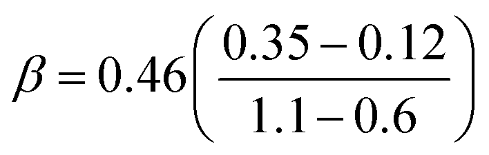, which we use to predict the free energy barrier for ER water formation between 0.35 V to 1.23 V, as shown in Fig. 5 (the lower limit is taken as 0.1 eV, the diffusion barrier for proton transfer). Thus we predict that

Fig. 5 Predicted activation energies (free energy barriers, ΔG^‡ in eV) for the rate determining steps from QM RμD calculations at various applied potentials, compared to experimental data (enthalpy, ΔH^‡ in eV). The theory suggests that ΔG^‡ = 0.25 eV for O* hydrolysis (solid green line) is rate determining below 0.87 V, while water formation via ER (solid black line) dominates at higher potential. The potential dependence of water formation (ER) was derived from the simulations at 0.6 V leading to ΔG^‡ = 0.12 eV and at 1.1 V leading to ΔG^‡ = 0.35 eV, leading to a slope of 0.46. The reaction barrier for proton transfer (∼0.1 eV) is taken as the lower limit for this step. The experimental data Exp 2 (red, Paulus et al. 2002)⁴⁸ and Exp 3 (blue, Grgur et al. 1997),⁴⁶ were determined by fitting to the Arrhenius equation the observed exchange current density (from the Tafel slope) over the temperature range 298–333 K. The results in Exp 1 (purple, Beattie et al. 1999)⁴⁵ may involve organic impurities from the Nafion solution. Note that the LH barrier of 0.29 eV for H* + *OOH reduction is reduced by the ER mechanism to below the 0.25 eV for O* hydrolysis for U > 0.

• for U < 0.87, ΔG^‡ = 0.25 eV (O* hydrolysis) a constant

• for U > 0.87. ΔG^‡ is determined by ER production of H₂O, which increases linearly to 0.41 eV at 1.23 V.

These results are in excellent agreement with experimental values from Markovic and coworkers^46,48 (based on fitting to the Arrhenius equation the exchange current density from the Tafel slope over the temperature range of 298–333 K).

• ΔG^‡ = 0.20 to 0.25 eV at U = 0.82 to 0.93 eV and

• ΔG^‡ = 0.44 eV at 1.23 V.

Other experimental studies using a Nafion electrolyte⁴⁵ obtained ΔG^‡ = 0.4 and 0.6 eV at U = 0.8. This significantly larger activation energy may be attributed to organic impurities from the Nafion solution, as explained by the authors.⁴⁵

Summarizing, we used QM based Reactive Molecular Dynamics at 298 K to predict the free energy barriers for ORR reactions on Pt(111) while including five layers of explicit water to simulate the water/Pt(111) interface. We corrected for the effect of the applied potential on the work function change during charge transfer for the various reaction steps to convert the constant electron QM results to constant potential QM. We find that the RDS has ΔG^‡ = 0.25 eV for U < 0.87, but it increases linearly to 0.41 at 1.23 V, in excellent agreement with experiment. An important discovery is that surface H₂O* plays an essential role in donating the H to various reaction steps, a non-electrochemical potential independent reaction (as suggested by Sha, Goddard, and coworkers).²⁵

With a validated mechanism in hand and a validated QM methodology, we can now consider how to modify these various steps can be by alloying, surface modification, changes in the electrolyte, etc. to further optimize the rates and overpotentials. Thus if the predicted potential dependent barrier of 0.41 eV at 1.23 V could be brought down to the potential independent value of 0.25, the rate for ORR would increase by a factor of 600 at 298 K, while allowing an operating over potential close to zero. This would most dramatically change the economics for fuel cells for transportation and utilize the chemical energy from solar fuel production.

Author contributions

T. C. and W. A. G. proposed the ideas; T. C., Q. A. and S. M. carried out the simulations; T. C. H. X. and B. M. analyzed the results, and the manuscript was written by T. C. and W. A. G.

Competing financial interests

The authors declare no competing financial interests.

Acknowledgements

This work was supported by National Science Foundation (CBET 1512759, program manager Robert McCabe). We thank Dr Ted Yu for helpful discussions.

References

1. W. Vielstich, H. Yokokawa and H. A. Gasteiger, Handbook of Fuel Cells: Fundamentals Technology and Applications, Wiley, 2009.
2. B. C. H. Steele and A. Heinzel, Nature, 2001, 414, 345–352.
3. M. Winter and R. J. Brodd, Chem. Rev., 2004, 104, 4245–4269.
4. K. P. Gong, F. Du, Z. H. Xia, M. Durstock and L. M. Dai, Science, 2009, 323, 760–764.
5. M. K. Debe, Nature, 2012, 486, 43–51.
6. H. A. Gasteiger, S. S. Kocha, B. Sompalli and F. T. Wagner, Appl. Catal., B, 2005, 56, 9–35.
7. J. A. Keith and T. Jacob, Angew. Chem., Int. Ed., 2010, 49, 9521–9525.
8. A. M. Gomez-Marin, R. Rizo and J. M. Feliu, Catal. Sci. Technol., 2014, 4, 1685–1698.
9. K. Kinoshita, Electrochemical Oxygen Technology, John Wiley & Sons, 1992.
10. A. Damjanovic, M. A. Genshaw and J. O. M. Bockris, J. Phys. Chem., 1966, 70, 3761–3762.
11. A. Damjanovic and V. Brusic, Electrochim. Acta, 1967, 12, 615–628.
12. S. Mukerjee, S. Srinivasan, M. P. Soriaga and J. McBreen, J. Electrochem. Soc., 1995, 142, 1409–1422.
13. X. Huang, Z. Zhao, L. Cao, Y. Chen, E. Zhu, Z. Lin, M. Li, A. Yan, A. Zettl, Y. M. Wang, X. Duan, T. Mueller and Y. Huang, Science, 2015, 348, 1230–1234.
14. L. Zhang, L. T. Roling, X. Wang, M. Vara, M. Chi, J. Liu, S.-I. Choi, J. Park, J. A. Herron, Z. Xie, M. Mavrikakis and Y. Xia, Science, 2015, 349, 412–416.
15. D. Wang, H. L. Xin, R. Hovden, H. Wang, Y. Yu, D. A. Muller, F. J. DiSalvo and H. D. Abruña, Nat. Mater., 2013, 12, 81–87.
16. S.-I. Choi, S. Xie, M. Shao, J. H. Odell, N. Lu, H.-C. Peng, L. Protsailo, S. Guerrero, J. Park, X. Xia, J. Wang, M. J. Kim and Y. Xia, Nano Lett., 2013, 13, 3420–3425.
17. V. R. Stamenkovic, B. Fowler, B. S. Mun, G. Wang, P. N. Ross, C. A. Lucas and N. M. Marković, Science, 2007, 315, 493–497.
18. A. Velázquez-Palenzuela, F. Masini, A. F. Pedersen, M. Escudero-Escribano, D. Deiana, P. Malacrida, T. W. Hansen, D. Friebel, A. Nilsson, I. E. L. Stephens and I. Chorkendorff, J. Catal., 2015, 328, 297–307.
19. P. Hernandez-Fernandez, F. Masini, D. N. McCarthy, C. E. Strebel, D. Friebel, D. Deiana, P. Malacrida, A. Nierhoff, A. Bodin, A. M. Wise, J. H. Nielsen, T. W. Hansen, A. Nilsson, E. L. StephensIfan and I. Chorkendorff, Nat. Chem., 2014, 6, 732–738.
20. K. Strickland, E. Miner, Q. Jia, U. Tylus, N. Ramaswamy, W. Liang, M.-T. Sougrati, F. Jaouen and S. Mukerjee, Nat. Commun., 2015, 6, 7343.
21. J. K. Nørskov, J. Rossmeisl, A. Logadottir, L. Lindqvist, J. R. Kitchin, T. Bligaard and H. Jónsson, J. Phys. Chem. B, 2004, 108, 17886–17892.
22. A. U. Nilekar and M. Mavrikakis, Surf. Sci., 2008, 602, L89–L94.
23. J. A. Keith, G. Jerkiewicz and T. Jacob, ChemPhysChem, 2010, 11, 2779–2794.
24. T. Jacob and W. A. Goddard, ChemPhysChem, 2006, 7, 992–1005.
25. Y. Sha, T. H. Yu, B. V. Merinov, P. Shirvanian and W. A. Goddard, J. Phys. Chem. Lett., 2011, 2, 572–576.
26. A. M. Gómez-Marín and J. M. Feliu, ChemSusChem, 2013, 6, 1091–1100.
27. N. M. Marković, R. R. Adžić, B. D. Cahan and E. B. Yeager, J. Electroanal. Chem., 1994, 377, 249–259.
28. J.-M. Noël, A. Latus, C. Lagrost, E. Volanschi and P. Hapiot, J. Am. Chem. Soc., 2012, 134, 2835–2841.
29. F. Tian and A. B. Anderson, J. Phys. Chem. C, 2011, 115, 4076–4088.
30. A. B. Anderson and T. V. Albu, J. Electrochem. Soc., 2000, 147, 4229–4238.
31. R. A. Sidik and A. B. Anderson, J. Electroanal. Chem., 2002, 528, 69–76.
32. H. A. Hansen, V. Viswanathan and J. K. Nørskov, J. Phys. Chem. C, 2014, 118, 6706–6718.
33. J. X. Wang, N. M. Markovic and R. R. Adzic, J. Phys. Chem. B, 2004, 108, 4127–4133.
34. A. Berná, V. Climent and J. M. Feliu, Electrochem. Commun., 2007, 9, 2789–2794.
35. M. Wakisaka, H. Suzuki, S. Mitsui, H. Uchida and M. Watanabe, Langmuir, 2009, 25, 1897–1900.
36. A. M. Gómez-Marín, J. Clavilier and J. M. Feliu, J. Electroanal. Chem., 2013, 688, 360–370.
37. V. Tripković, E. Skúlason, S. Siahrostami, J. K. Nørskov and J. Rossmeisl, Electrochim. Acta, 2010, 55, 7975–7981.
38. H. S. Casalongue, S. Kaya, V. Viswanathan, D. J. Miller, D. Friebel, H. A. Hansen, J. K. Nørskov, A. Nilsson and H. Ogasawara, Nat. Commun., 2013, 4, 2817.
39. M. Ding, Q. He, G. Wang, H.-C. Cheng, Y. Huang and X. Duan, Nat. Commun., 2015, 6, 7867.
40. Y. Sha, T. H. Yu, Y. Liu, B. V. Merinov and W. A. Goddard, J. Phys. Chem. Lett., 2010, 1, 856–861.
41. J. A. Herron, Y. Morikawa and M. Mavrikakis, Proc. Natl. Acad. Sci. U. S. A., 2016, 113, E4937–E4945.
42. C. D. Taylor, S. A. Wasileski, J.-S. Filhol and M. Neurock, Phys. Rev. B: Condens. Matter Mater. Phys., 2006, 73, 165402.
43. M. J. Janik, C. D. Taylor and M. Neurock, J. Electrochem. Soc., 2009, 156, B126–B135.
44. L. Sementa, O. Andreussi, W. A. Goddard III and A. Fortunelli, Catal. Sci. Technol., 2016, 6, 6901–6909.
45. P. D. Beattie, V. I. Basura and S. Holdcroft, J. Electroanal. Chem., 1999, 468, 180–192.
46. B. N. Grgur, N. M. Marković and P. N. Ross, Can. J. Chem., 1997, 75, 1465–1471.
47. A. B. Anderson, J. Roques, S. Mukerjee, V. S. Murthi, N. M. Markovic and V. Stamenkovic, J. Phys. Chem. B, 2005, 109, 1198–1203.
48. U. A. Paulus, A. Wokaun, G. G. Scherer, T. J. Schmidt, V. Stamenkovic, V. Radmilovic, N. M. Markovic and P. N. Ross, J. Phys. Chem. B, 2002, 106, 4181–4191.
49. J. Ludwig, D. G. Vlachos, A. C. T. van Duin and W. A. Goddard, J. Phys. Chem. B, 2006, 110, 4274–4282.
50. J. Carrasco, A. Hodgson and A. Michaelides, Nat. Mater., 2012, 11, 667–674.
51. H. Ogasawara, B. Brena, D. Nordlund, M. Nyberg, A. Pelmenschikov, L. G. M. Pettersson and A. Nilsson, Phys. Rev. Lett., 2002, 89, 276102.
52. N. Markovic, H. Gasteiger and P. N. Ross, J. Electrochem. Soc., 1997, 144, 1591–1597.
53. K. Chan and J. K. Nørskov, J. Phys. Chem. Lett., 2016, 7, 1686–1690.

---

Footnote

† Electronic supplementary information (ESI) available: Simulation methods, Fig. S1–S7, Table S1 and ref. 49–59. See DOI: 10.1039/c6cp08055c

---