
 Open Access Article
 This Open Access Article is licensed under a Creative Commons Attribution-Non Commercial 3.0 Unported Licence
Local order drives the metallic state in PEDOT:PSS†
Philipp
Stadler
*a,
Dominik
Farka
a,
Halime
Coskun
a,
Eric D.
Głowacki
a,
Cigdem
Yumusak
a,
Lisa M.
Uiberlacker
b,
Sabine
Hild
b,
Lucia N.
Leonat
c,
Markus C.
Scharber
a,
Petr
Klapetek
d,
Reghu
Menon
e and
N. Serdar
Sariciftci
a
aInstitute of Physical Chemistry, Johannes Kepler University Linz, Altenbergerstr. 69, 4040 Linz, Austria. E-mail: philipp.stadler@jku.at; Fax: +43 732 2468 1213; Tel: +43 732 2468 8770
bInstitute of Polymer Science, Johannes Kepler University Linz, Altenbergerstr. 69, 4040 Linz, Austria
cThe National Institute for Electrical Engineering, ICPE-CA, Splaiul Unirii 313, 030138 Bucharest, Romania
dCentral European Institute of Technology, Koliste 13a, 602 00 Brno, Czech Republic
eDepartment of Physics, Indian Institute of Science, Bangalore 560012, India
First published on 23rd June 2016
Abstract
Weak localization describes a metallic system, where due to the presence of disorder the electrical transport is governed by inelastic electron relaxation. Therefore the theory defines a threshold of spatial and of energetic disorder, at which a metal–insulator transition takes place. To achieve a metallic state in an inherently disordered system such as a conductive polymer, one has to overcome the threshold of localization. In this work we show that the effective suppression of disorder is possible in solution-processible poly(3,4-ethylenedioxythiophene)–poly(styrene sulfonate). We grow polymer films under optimized conditions allowing self-organization in solution. Interestingly, we find the requisite threshold, at which the system becomes finally metallic. We characterize the transition using a complementary morphology and magneto-electrical transport study and find coherent electron interactions, which emerge as soon as local order exceeds the macromolecular dimensions. These insights can be used for discrete improvement in the electrical performance, in particular for tailoring conductive polymers to alternative metal-like conductors.
1 Introduction
The generation of an intrinsically metallic conductive polymer (CP) is one of the primary goals in developing powerful organic and bio-organic electronics.1–7 However, the question, when a CP is regarded as metallic, has caused ambiguous discussions.1,2,5,8–10 This relates to the fact that CPs are highly anisotropic – their solid state structure reflects a mutual interplay of different interactions: a polymer strain is covalently connected along the chain direction, while between the adjacent macromolecules stacking forces are dominant. Finally, conductive polymers also have a strong ionic character, as in the doped form, (delocalized) carriers on the polymer chain are counterbalanced by immobile ions. Furthermore, the polymers themselves are prone to condense dispersively with alternating amorphous and crystalline regions. Taking these views into consideration the formation of a metallic state appears to be strongly dependent on the local order – accepting the fact that some disorder is inherently present. This is an important information, as even classic metals change their electrical transport drastically in the presence of disorder. The physics are therefore described by weak localization (WL).11 WL specifies a system in the presence of disorder, when the electrical transport is governed by inelastic scattering processes. This translates to a change in the sign of the temperature coefficient of the conductivity to a positive value. At low temperatures, a minimum is reached – Mott's minimum conductivity, σmin. At this point inelastic and elastic processes are equally present. In practice, the σmin for CPs is close to T = 0 and therefore experimentally difficult to observe. We therefore shift our attention to the mean inelastic electron scattering lengths, which can be measured above σmin to obtain a direct insight of the local order.12–15 With this information it is possible to resolve the ambiguity of the electrical transport in conductive polymers. Shedding light on the inelastic scattering processes allows us to resolve the metal–insulator-transitions as described by Mott and Anderson.16,17 In this work we harness the great potential of self-organization in solution and set up an experimental study to demonstrate finally the metallic state established by the subsequent local order. This represents the crucial ingredient needed to drive the metallic state – even in systems having at first sight a moderate conductivity at room temperature. The experimental path towards the metal–insulator-transition and the fundamental insight into the electron scattering is presented in detail.
2 Sample growth, measurement techniques and characteristics
We apply a facile route via supramolecular self-organization in solution to intrinsically achieve the metallic state in poly(3,4-ethylenedioxythiophene):polystyrenesulfonate (PEDOT:PSS) with alternating concentrations of dimethylsulphoxide (DMSO) and alternating thickness. The films are prepared from the original commercial dispersion (PH1000, Heraeus) using 4 main recipes with various intermediate blends: no DMSO (ref), 2% (i.e. 20 μl per ml volume), 5% and 10% DMSO, both spin-coating and drop-casting. The dispersion is vigorously stirred at 60 °C overnight. For the thicker films we used drop-casting with variable volumes of the dispersion (1 ml to 0.1 ml) dropped on a glass wafer (2.54 × 2.54 cm2), which is dried at 60 °C for 2 h. The as-gained films (1 to 10 mm) are elevated from the glass and dried once more in an inert atmosphere over CaH2 at 100 °C. For the thin-films the dispersion is spin-cast using various recipes to obtain thin-film systems ranging from 10 nm up to 100 nm. All films are subsequently dried for 3 days in an inert atmosphere to remove residual DMSO and water. The free-standing bulk films are cut to rectangular 1.5 × 10 mm2 slices and contacted with gold-patterns in vacuo as shown in the photograph (Fig. 5D) and mounted on the cryomagnet system, so that the B-field is perpendicular to the film plane (Bz). In a similar manner, as cast thin-films on sapphire are contacted directly by as-deposited gold. We denote that due to the change in the processing steps between thicker and thinner films, we find minor thickness-effect on the electrical performance (see Fig. 1A and B). Finally, the voltage drop across the inner leads is measured (at Ix = 50 μA) as a function of T and B-fields. The metallic film picks are characterized further by repeating scans for conductivity and magneto-conductivity, respectively. Similarly, for the XRD spectra the films are cut into 1 × 1 cm2 squares and analyzed using a Bruker AXS diffractometer equipped with a CuKα source. For the atomic force microscopy (AFM), the bulk-films are cut with a Leica Ultracut microtome and the polished cross-sections are analyzed using a Asylum Research MFP-3D Stand Alone AFM. The thin-films are analyzed directly on the surface as grown on the sapphire substrate.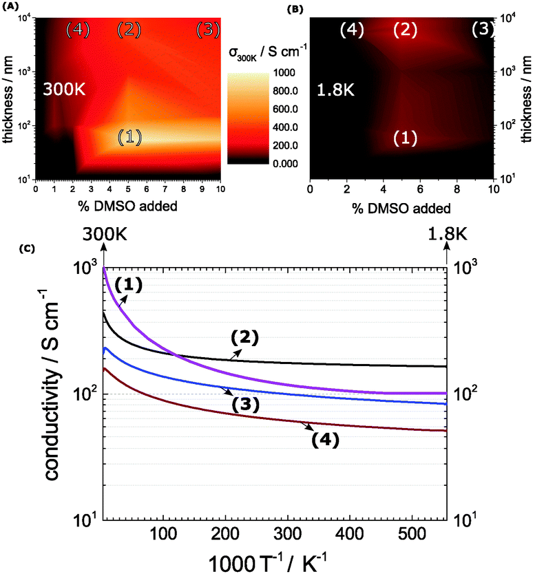 | ||
| Fig. 1 (A) Room-temperature mapping of PEDOT:PSS conductivities at different DMSO-concentrations and thicknesses. (B) Repeats the map at 1.8 K. (C) The temperature profiles of the conductivities are significantly different between bulk and thin-films. The in detail study systems are highlighted in the map at 55 nm and 5% DMSO (1), 8.4 μm and 5% DMSO (2), 8.4 μm and 10% DMSO (3) and finally 8.4 μm and 2% DMSO (4). | ||
3 Results and discussion
The casting process for PEDOT:PSS has been investigated in detail earlier – in particular the co-solvent treatment has lead to substantial improvements in the conductivities.4,10,18–21 An established pair represents PEDOT:PSS and DMSO as co-solvent.20,22–24 This is the system of choice in this work.We start with a number of thin-film PEDOT:PSS recipes yielding 10 nm thickness and successively increase the width to access a more and more bulk phase up to 10 mm. In addition we modify the co-solvent present between 0 and 10% of the original volume dispersion. Our goal is to attain a detailed insight of the co-solvent concentration and of the final film thickness into the resulting conductivities (Fig. 1A). We consistently find excellent electrical performances at DMSO concentrations around 5%. Here we achieve peak conductivities of 1000 S cm−1 at a thickness of 55 nm as seen in the map in Fig. 1A denoted further as (1). The effect is less pronounced at lower and higher DMSO concentrations, which is in agreement with previous studies.22,23
When the film thickness expands to a bulk system greater than 1 μm we see a similar increase of the electrical performance on the DMSO concentration. Nonetheless, the bulk-films achieve a maximum of 490 S cm−1 at 5% DMSO and 8.4 μm respectively (2). So the map in Fig. 1A exhibits a consistent out-performance of thin-films over bulk films. Other detailed studied systems are 10% DMSO and 8.4 μm (3) and 2% DMSO and 8.4 μm (4).
When we repeat the mapping at 1.8 K we obtain a first insight, where in the map the local order allows the formation of a metallic state (Fig. 1B). According to Mott's minimum conductivity, regions off the metallic regime exhibit an infinite low conductivity, which is valid for the preponderant dark regions seen in the 1.8 K map. Regimes in proximity to a metal–insulator transition (MIT) appear still conductive – they are found in the same hotspots as at room temperature with an important changeover: at 1.8 K, the bulk systems outperform the thin-films. The reason for this lies in the pronounced temperature-dependence of the thin film conductivities. Meanwhile, the bulk film conductivities exhibit a moderate temperature-profile in agreement with weak localization with a flattening as the temperature approaches 0 (Fig. 1C).
In combination, the maps show us the optimum region, which lies between 2 and 5% DMSO and 8.4 μm layer thickness (2) and (4). At 5% DMSO and 1.8 K, for example, the bulk-conductivity (2) exceeds the 55 nm thin-film (1) conductivity by a factor of nearly 2. This minor temperature-sensitivity points out that the thickness plays a role in terms of local order – it relates to the different parameters in the processing and to a suppressed substrate-effect in the bulk-systems. To support our findings from the conductivity maps we view the morphologies by AFM and XRD, in particular in the optimum region (Fig. 2).
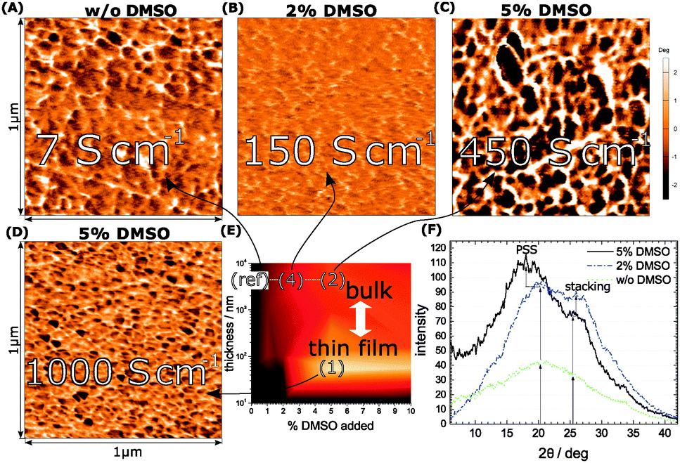 | ||
| Fig. 2 In panels (A–C) the cross-sectional morphologies by AFM of no DMSO (ref), (4) and (2) are shown. In (D) the morphology of (1) by AFM is depicted (surface scan). (E) Conductivity map at 1.8 K. The XRD-spectra in (F) highlight the improved crystallinity in (4) and (2) as compared to (ref) by increasing the DMSO concentration during film-growth. | ||
For the bulk films we plot the XRD spectra at no (ref), 2% (4) and 5% DMSO (2). A sharpened profile in terms of crystallinity correlates with the presence of DMSO during growth.25,26 (Fig. 2E). In general the increase of the electrical conductivity from Fig. 1A is reflected in a pronounced signal, which underlines the higher degree of crystallinity. The discrete peak originating from the π-stacking of PEDOT emerges at 25 deg. It is overlapped by the broad response of the PSS halo with a maximum at 20 deg. The spectral shaping through DMSO consequently supports our argument of improved crystallization in the presence of DMSO valid for both components, PEDOT and PSS, respectively. To clarify, we present a comparison of PEDOT and regio-regular poly(-3-hexylthiophene) (rr-P3HT) grown under similar conditions in the ESI.† A supplementary view of the morphological changes induced by DMSO is outlined by atomic force microscopy (AFM). As shown in the phase images in Fig. 2A–D we find different grain sizes at each representative (conductivity) area (marked as a white rectangular frame) from the conductivity map (Fig. 2E). Fig. 2D depicts the thin-film phase image revealing a randomized distribution of structured domains with different grain sizes. This is reminiscent to the bulk-film without DMSO, where polydispersity is detected again. Obviously, the presence of small amounts of DMSO (2%) and thicker films (4) improves the homogeneity a lot as shown in Fig. 2B, where the grains of the structure become smaller. To achieve a growing grain size and a homogeneous dispersion the concentration has to be further increased to 5% (2), where we find the point of merit in terms of conductivity, crystallinity and morphology in the bulk-films. We denote that we derive the bulk-film morphology from cross-sectional scans in order to allow a meaningful comparison between bulk and thin-film morphologies.
The morphology response of the different conductivity-stages reveals the importance of long-range order plus the role of dispersivity seen in growing ordered domains of similar size, which explains the improved electrical performance at low-T.
Back in Fig. 1 we outline the positive temperature coefficient  with finite conductivity as T approaches 0 best seen in (4), (1) and (2). This behaviour corresponds to weak localization. To resolve the low-T regime, we use the derivative of the conductivity in the logarithmic scale
  further denoted as W.27
The metallic character is expressed by the slope and magnitude of W(T). As seen in Fig. 3 the system without DMSO (ref) shows a constant W with quantities greater than 1 (insulating regime). In contrast, (4), (1) and (2) deviate − W(T) is not constant. In particular, at low temperature it illustrates that on which side of the MIT the system is situated. In the case of bulk 5% DMSO (2), the slope of W(T) becomes positive indicating a metallic state (Fig. 3B). We denote that in particular the thin-film response from (1) shows a clear non-metallic fingerprint at low-T, which we assign to the role of dispersivity.
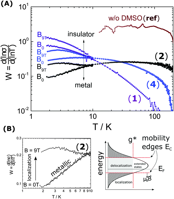 | ||
Fig. 3 (A) Highlights the exponent of the power-law dependence  (W), in particular at low temperatures (T ≤ 10 K) and high magnetic field (B = 9 T). While the first sample (no DMSO) (ref) operates beyond the transition line at W = 1, we see a shift towards a metal in (1), (2) and (4) and high B-field localization resulting in a negative magnetoconductivity. (W), in particular at low temperatures (T ≤ 10 K) and high magnetic field (B = 9 T). While the first sample (no DMSO) (ref) operates beyond the transition line at W = 1, we see a shift towards a metal in (1), (2) and (4) and high B-field localization resulting in a negative magnetoconductivity. | ||
The proximity of the metallic state can be tested by applying a high magnetic field perpendicular to the substrate plane (Bz = 9 T). The field induces localization and quenches the metallic state as shown in Fig. 3. A substantial change in W(T) by B is therefore seen below 10 K. There W splits up into a critical-metallic (B = 0 T) and non-metallic regime (B = 9 T). This is true for both (4) and (2) (only for the bulk systems), where a shallow metallic behaviour is observed at T below 10 K.
So far, we have created a system with sufficient local order. We prove the metallic behaviour in the bulk samples between 1.8 K and 10 K seen by W(T) in Fig. 3B. In addition we demonstrate that a high magnetic fields can disrupt the local order of a metallic state, in particular at low temperatures.
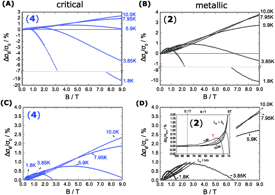
When we take the view to the lower B-field, interestingly we find a concomitantly stimulating effect on the metallic character in our samples of merit (2 and 4). In contrast to Fig. 3 low B-fields enhance the conductivity. A detailed view of the magnetoconductivity 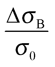 as a function of B shows this positive contribution (Fig. 4).
 | ||
| Fig. 4 (A) 2% (4) and (B) 5% DMSO-cast (2) PEDOT:PSS systems reflect the interplay between positive and negative magnetoconductivity (MC) at low T. For each T the positive effects dominate first at low B followed by a flip to the negative by increasing B (at 1.8 K, 3.85 K and 5.9 K). At higher T (7.95 and 10.0 K) the MC is only positive. We denote that the negative effect is more pronounced in the critical sample. In (C) and (D) we expand the positive side and show the semicircular development of each MC with B. In the metallic sample (1) we depict its MC as a function of the Landau orbit size LD in addition to show the interference under resonance conditions, when the mean inelastic scattering length λε and LD are of similar dimension (inset). | ||
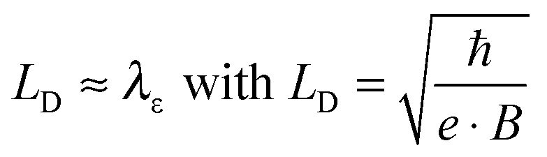
We observe the conductivity increasing up to 4% of the original value. It is followed by a significant decrease to the negative as the field is increased. The negative effect is damped at high temperatures, where the turn to the negative is indicated at high B and not seen at all at temperatures above 6 K. One explanation for magnetic stimulation relates to a electro-magnetic resonance, earlier found in systems defined by weak localization: In fact, the stimulation reflects an interaction among the electron wave functions, as soon as the inelastic mean free path of electrons λε and the Landau orbit size LD.28–30 become comparable.
 | (1) |
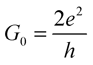
Eqn (1) depicts the relation of LD (or B) and of λε (Fig. 4). At 1.8 K, for example, the ΔσB-value increases up to 1 T (2), before it collapses to the negative by increasing B (Fig. 4C and D). The peak maximum of ΔσB corresponds to the amplitude of the local order or λε, respectively. It can be consequently read out by plotting LD instead of B. A similar but right-shifted profile is observed at 3.85 K. At higher temperatures the stimulations do not collapse meaning that λε exceeds the maximum field at Bmax = 9 T or LD = 8.1 nm according to eqn (1), as λε decreases below the maximum magnetic field as we increase the temperature. Positive magnetoconductivity has been reported solely in combination with metallic samples – it reveals a coherence among electron wave functions and B.28,30–37 In our case this is supported by the morphology study (homogeneous domains of similar size, Fig. 3). Other theories assign the stimulating magneto-effect to the spin–orbit coupling. However, in organic matter these effects can be neglected.11 We use the coherent electron interactions as a direct consequence of long-range order inside the polymer. To quantitatively evaluate the magnetoconductivity, we derive concrete values for λε statistical parameters to visualize the local order. Kawabata has posted a relation between magnetoconductivity and the relaxation time (hence the mean free path λε).28 We can derive the magnitude by plotting + σBversus B2 according to
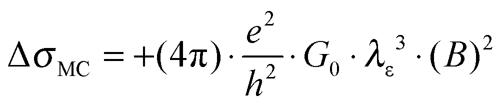 | (2) |
 . The corresponding Fig. 5 shows the temperature-variant slopes and the accompanying linear fits for each temperature. In the best case in (2) the electron coherence quantitatively translates to a scattering length of 35.5 nm at 1.8 K. This value exceeds the macromolecular dimensions and explains the metallic fingerprint of the system. We summarized all relevant parameters in Table 1. With the T)−¾)vs. λε plot in Fig. 5C we include the temperature-dependence with the exponent 0.75 typical for inelastic scattering.29 The dimensions of λε are exponentially decreasing by increasing the temperature – as we go off the metallic regime, we observe a deviation as visible in the critically transition regime in (4).
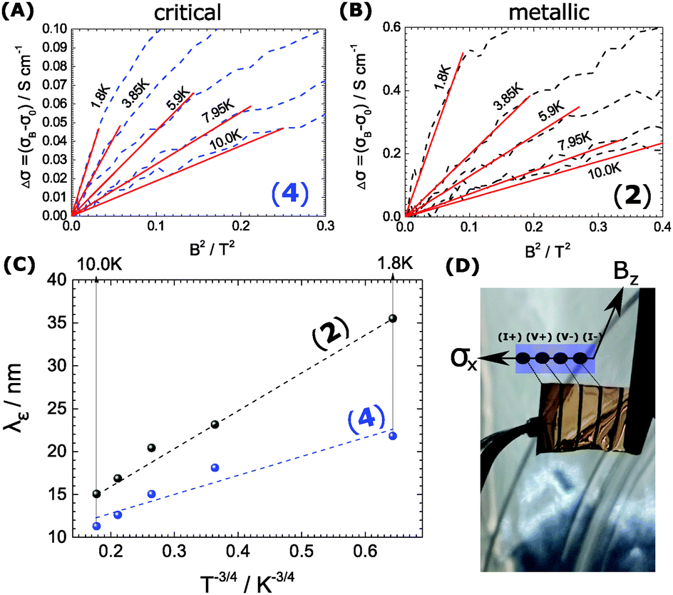 | ||
| Fig. 5 (A and B) Depict the linear dependence of the magnetoconductivity ΔσB and B2 at low fields in the samples of merit (2) and (4). The slope (linear fit) is proportional to the mean inelastic scattering length λε. (C) Shows the T-dependence of λε. For inelastic scattering an exponent of −¾ is typical. This is only the case in the metallic 5% DMSO sample (2). (D) Depicts the sample (free-standing PEDOT:PSS film with 4 Au leads) ready for loading into the cryomagnet. | ||
| Label | Thickness/nm | % DMSO | σ 300K/S cm−1 | σ 1.8K/S cm−1 | Ratio σ300K/σ1.8K | λ ε/nm (at 1.8 K) |
|---|---|---|---|---|---|---|
| (ref) | 8400 | 0 | 7.1 | N/A | N/A | N/A |
| (1) | 55 | 5 | 1000 | 101.5 | 9.83 | N/A |
| (2) | 8300 | 5 | 490 | 170 | 2.54 | 35.5 |
| (3) | 9200 | 10 | 275 | 80 | 3.42 | N/A |
| (4) | 8300 | 2 | 155 | 50 | 2.96 | 21.8 |
4 Conclusions
We underline here the value of magnetoconductivity to display local order, which is crucial to establish a metallic state in a conductive polymer. The order can be surfaced by the coherent transport and represents a strong argument for achieving a metallic state. We show that it is possible to improve on the electrical performance, when the morphology becomes homogeneous and locally ordered. This is demonstrated by expanding the sample's dimension towards a bulk-phase and by allowing self-organization. Thus our strategy can be a model system for various CP-systems to strengthen their electrical transport properties towards an intrinsically-metallic, alternative conductor.Acknowledgements
This work has been supported by the OEAD (WTZ, IN10/2015) and the Austrian Fund for Advancement of Science (FWF) within the Wittgenstein Prize scheme (Z222-N19 Solare Energieumwandlung).References
- K. Lee, S. Cho, S. Heum Park, A. J. Heeger, C.-W. Lee and S.-H. Lee, Nature, 2006, 441, 65–68 CrossRef CAS PubMed.
- Y. H. Kim, C. Sachse, M. L. Machala, C. May, L. Müller-Meskamp and K. Leo, Adv. Funct. Mater., 2011, 21, 1076–1081 CrossRef CAS.
- D. Alemu Mengistie, P.-C. Wang and C.-W. Chu, J. Mater. Chem. A, 2013, 1, 9907 CAS.
- O. Bubnova, Z. U. Khan, H. Wang, S. Braun, D. R. Evans, M. Fabretto, P. Hojati-Talemi, D. Dagnelund, J.-B. Arlin, Y. H. Geerts, S. Desbief, D. W. Breiby, J. W. Andreasen, R. Lazzaroni, W. M. Chen, I. Zozoulenko, M. Fahlman, P. J. Murphy, M. Berggren and X. Crispin, Nat. Mater., 2013, 13, 190–194 CrossRef PubMed.
- D. A. Mengistie, P.-C. Wang and C.-W. Chu, ECS Trans., 2013, 58, 49–56 CrossRef.
- N. Massonnet, A. Carella, A. de Geyer, J. Faure-Vincent and J.-P. Simonato, Chem. Sci., 2015, 6, 412–417 RSC.
- E. Stavrinidou, R. Gabrielsson, E. Gomez, X. Crispin, O. Nilsson, D. T. Simon and M. Berggren, Sci. Adv., 2015, 1, e1501136 Search PubMed.
- J. Huang, P. Miller, J. de Mello, A. de Mello and D. Bradley, Synth. Met., 2003, 139, 569–572 CrossRef CAS.
- Y. Xia, K. Sun and J. Ouyang, Adv. Mater., 2012, 24, 2436–2440 CrossRef CAS PubMed.
- B. J. Worfolk, S. C. Andrews, S. Park, J. Reinspach, N. Liu, M. F. Toney, S. C. B. Mannsfeld and Z. Bao, Proc. Natl. Acad. Sci. U. S. A., 2015, 112, 14138–14143 CrossRef CAS PubMed.
- G. Bergmann, Phys. Rep., 1984, 107, 1–58 CrossRef CAS.
- S. D. Baranovskii, Phys. Status Solidi B, 2014, 251, 487–525 CrossRef CAS.
- H. C. F. Martens, J. A. Reedijk, H. B. Brom, D. M. de Leeuw and R. Menon, Phys. Rev. B: Condens. Matter Mater. Phys., 2001, 63, 073203 CrossRef.
- A. Aleshin, R. Kiebooms, R. Menon and A. Heeger, Synth. Met., 1997, 90, 61–68 CrossRef CAS.
- R. Menon, C. O. Yoon, D. Moses, A. J. Heeger and Y. Cao, Phys. Rev. B: Condens. Matter Mater. Phys., 1993, 48, 17685–17694 CrossRef CAS.
- P. W. Anderson, Phys. Rev., 1958, 109, 1492–1505 CrossRef CAS.
- N. F. Mott, Philos. Mag., 1972, 26, 1015–1026 CrossRef CAS.
- S. Jönsson, J. Birgerson, X. Crispin, G. Greczynski, W. Osikowicz, A. Denier van der Gon, W. Salaneck and M. Fahlman, Synth. Met., 2003, 139, 1–10 CrossRef.
- O. Bubnova, Z. U. Khan, A. Malti, S. Braun, M. Fahlman, M. Berggren and X. Crispin, Nat. Mater., 2011, 10, 429–433 CrossRef CAS PubMed.
- J. Gasiorowski, R. Menon, K. Hingerl, M. Dachev and N. S. Sariciftci, Thin Solid Films, 2013, 536, 211–215 CrossRef CAS PubMed.
- X. Crispin, F. L. E. Jakobsson, A. Crispin, P. C. M. Grim, P. Andersson, A. Volodin, C. V. Haesendonck, M. V. D. Auweraer, W. R. Salaneck and M. Berggren, Chem. Mater., 2006, 18, 4354–4360 CrossRef CAS.
- I. Cruz-Cruz, M. Reyes-Reyes, M. Aguilar-Frutis, A. Rodriguez and R. López-Sandoval, Synth. Met., 2010, 160, 1501–1506 CrossRef CAS.
- C. Pathak, J. Singh and R. Singh, Curr. Appl. Phys., 2015, 15, 528–534 CrossRef.
- T.-R. Chou, S.-H. Chen, Y.-T. Chiang, Y.-T. Lin and C.-Y. Chao, J. Mater. Chem. C, 2015, 3, 3760–3766 RSC.
- Q. Wei, M. Mukaida, Y. Naitoh and T. Ishida, Adv. Mater., 2013, 25, 2831–2836 CrossRef CAS PubMed.
- C. M. Palumbiny, F. Liu, T. P. Russell, A. Hexemer, C. Wang and P. Müller-Buschbaum, Adv. Mater., 2015, 27, 3391–3397 CrossRef CAS PubMed.
- E. B. Aleksandrov, I. V. Sokolov, A. Gatti, M. Kolobov, L. Lugiato and T. Vartanyan, Usp. Fiz. Nauk, 2001, 171, 1263 Search PubMed.
- A. Kawabata, Solid State Commun., 1980, 34, 431–432 CrossRef CAS.
- P. A. Lee and T. V. Ramakrishnan, Rev. Mod. Phys., 1985, 57, 287–337 CrossRef CAS.
- A. B. Kaiser, Rep. Prog. Phys., 2001, 64, 1 CrossRef CAS.
- B. Chapman, R. G. Buckley, N. T. Kemp, A. B. Kaiser, D. Beaglehole and H. J. Trodahl, Phys. Rev. B: Condens. Matter Mater. Phys., 1999, 60, 13479–13483 CrossRef CAS.
- F. Pikus and G. Pikus, Solid State Commun., 1996, 100, 95–99 CrossRef CAS.
- T. F. Rosenbaum, R. F. Milligan, G. A. Thomas, P. A. Lee, T. V. Ramakrishnan, R. N. Bhatt, K. DeConde, H. Hess and T. Perry, Phys. Rev. Lett., 1981, 47, 1758–1761 CrossRef CAS.
- R. Menon, K. Väkiparta, Y. Cao and D. Moses, Phys. Rev. B: Condens. Matter Mater. Phys., 1994, 49, 16162–16170 CrossRef.
- Y. Nogami, H. Kaneko, H. Ito, T. Ishiguro, T. Sasaki, N. Toyota, A. Takahashi and J. Tsukamoto, Phys. Rev. B: Condens. Matter Mater. Phys., 1991, 43, 11829–11839 CrossRef CAS.
- H. H. S. Javadi, A. Chakraborty, C. Li, N. Theophilou, D. B. Swanson, A. G. MacDiarmid and A. J. Epstein, Phys. Rev. B: Condens. Matter Mater. Phys., 1991, 43, 2183–2186 CrossRef CAS.
- G. Bergmann, Phys. Rev. B: Condens. Matter Mater. Phys., 1983, 28, 2914–2920 CrossRef CAS.
Footnote |
| † Electronic supplementary information (ESI) available. See DOI: 10.1039/c6tc02129h |
| This journal is © The Royal Society of Chemistry 2016 |