
 Open Access Article
 This Open Access Article is licensed under a
 Creative Commons Attribution 3.0 Unported Licence
Simulation insights into the role of antiparallel molecular association in the formation of smectic A phases
Martin
Walker
 and
Mark R.
Wilson
*
and
Mark R.
Wilson
*
Durham University, Department of Chemistry, Lower Mountjoy, South Road, Durham DH1 3LE, UK. E-mail: mark.wilson@durham.ac.uk; Tel: +44 (0) 191 384 1158
First published on 29th September 2016
Abstract
A simple dissipative particle dynamics (DPD) model is introduced, which can be used to represent a broad range of calamitic mesogens. The model allows for antiparallel association that occurs naturally in a number of mesogens with terminal dipoles, including the 4-n-alkyl-4′-cyanobiphenyl (nCB) series. Favourable antiparallel interactions lead to the formation of SmAd phases in which the layer spacing is intermediate between monolayer and bilayer. The model is easily tuned to vary the strength of antiparallel association and the SmA layer spacing, and to give either isotropic–smectic or isotropic–nematic–smectic phase sequences. The model allows for a range of other smectics: including SmA1 phases exhibiting microphase separation within layers, and smectics A structures with more complicated repeat units. For large system sizes (≥50![[thin space (1/6-em)]](https://www.rsc.org/images/entities/char_2009.gif) 000 molecules) in the nematic phase, we are able to demonstrate the formation of three distinct types of cybotactic domains depending on the local interactions. Cybotactic domains are found to grow in the nematic–smectic pretransitional region as the system moves closer to TSN.
000 molecules) in the nematic phase, we are able to demonstrate the formation of three distinct types of cybotactic domains depending on the local interactions. Cybotactic domains are found to grow in the nematic–smectic pretransitional region as the system moves closer to TSN.
1 Introduction
Thermotropic liquid crystals represent a fascinating area of soft matter science. High interest arises from the wide range of different liquid crystal mesophases that have been produced by Chemists; and also from the large number of commercial applications. The former includes new forms of nematic phase,1 and a preponderance of smectic phases of varying degrees of translation and rotational order.2 Applications cover the areas of thermochromic materials,3 lasers,4 high-tech lubricants,5 liquid crystal displays,6 and a range of optoelectronic applications such as optical filters and switches, beam-steering devices and spatial light modulators.7Molecular simulations have proven to be critical in explaining some of the fundamental aspects of liquid crystal phase behaviour.8,9 Early simulation studies used simple hard repulsive shapes to model liquid crystal molecules, e.g. spherocylinders to represent prolate molecules10,11 and cut disks to represent oblate molecules.12 Hard potentials were able to generate simple phase diagrams with isotropic, nematic and smectic phases, employing only an entropic contribution to the total free energy. As computational power increased the development of anisotropic-attractive-coarse-grained models, such as the Gay-Berne potential,13–15 led to increased use of simulations to explore the link between molecular structure, phase behaviour and the bulk properties of liquid crystal phases.16–18 For nematics, it is now possible to generate very good predictions for transition temperatures from atomistic simulations of liquid crystal phases.19–21 However, for more complex mesophases, coarse-grained models are extremely useful; particularly because the system sizes and time scales required are usually too demanding for atomistic level models.
While excluded volume factors play a major role in driving mesophase formation, specific pair-wise interactions have long been known to provide an important contribution to the formation of some liquid crystal phases.22–24 Moreover, subtle effects such as changes in the tilt angle within smectic C liquid crystals, and re-entrant phase behaviour can be attributed to specific (often dipole–dipole coupling) interactions.25
The layer structure of a number of smectic liquid crystals is also influenced by dipole–dipole coupling interactions. For example, 4-n-octyl-4′-cyano-biphenyl, 8CB, which has a large dipole at the end of the molecule, adopts a smectic-A phase (classified as SmAd), in which the layer spacing, dlayer = 1.4 molecular lengths.26–28 The extended layer spacing is attributed to a preferred antiparallel packing of molecules,29,30 predominately driven by antiparallel dipole–dipole ordering. Atomistic simulations have been able to reproduce both the dipole–dipole ordering and the layer spacing in 8CB,20,31,32 albeit for a small number of smectic layers (on account of system size limitations). The simulations show that the layer density wave is considerably broader than that observed in other smectic A phases. Moreover, despite the fact that other parts of the molecular interaction have a far stronger influence on transition temperatures than dipole–dipole interactions, the latter are vital in determining the overall structure of the phase.
The SmAd phase of 8CB is only one of the possible smectic A phases that can occur when there is competition between two competing incommensurate lengths: that of a molecule and that of a pair of molecules. de Gennes and Prost show, with a Landau theory of frustrated smectics,33 how this can lead to a series of different smectics A phases with different density waves: SmA1 (monolayer), SmA2 (bilayer), SmAd and SmÃ.
In this paper, we present a coarse-grained dissipative particle dynamics (DPD) model for liquid crystal molecules, in which the effects of specific molecular interactions (such as those leading to dipole–dipole correlation or to microphase separation in smectics) can be incorporated easily. We show that we can represent nematic and smectic SmAd phases within the model (mimicking the behaviour of 8CB); and we show how a wide range of smectic-A phases can be generated by tuning the local interaction potential to favour specific interactions leading to local (dynamic) molecular recognition. We show also that DPD (because of the large system sizes and time scales possible) provides a valuable tool for looking at pretransitional fluctuations and cybotactic behaviour within nematic systems.
2 Computational methods
Originally designed for block co-polymer systems, DPD has a smooth repulsive potential that allows for a relatively large time step. Coupling the reduced degrees of freedom of a coarse grained simulation with a large time step has enabled simulation of a wide range of soft matter: block co-polymers,34–36 colloidal suspensions,37 lipid bilayers,38,39 nanoparticles,40,41 and liquid crystalline phases,42,43 where the hydrodynamic time-scale can become important. Molecular systems are readily coarse-grained to a DPD representation, replacing multiple atoms or chemical groups with single-site beads. Different interactions can be represented by adjusting the DPD conservative force constant aij (see below), and this has been used to good effect in simulating polyphilic molecules such as bolaamphiphiles.44–48 Here, we simulate preferred antiparallel molecular interactions by using two sites, B and C, which have a preferred B–C interaction.In DPD three simple forces act on the system: a conservative force, FC, a dissipative force, FD, and a random force, FR.
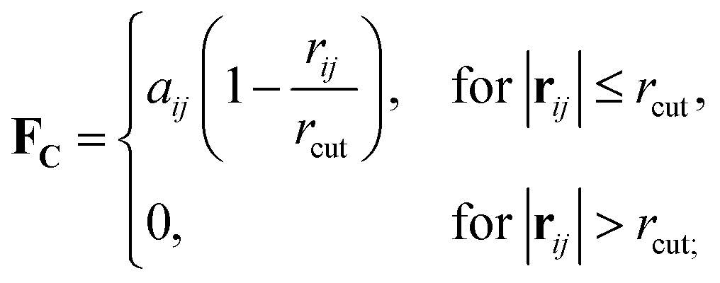 | (1) |
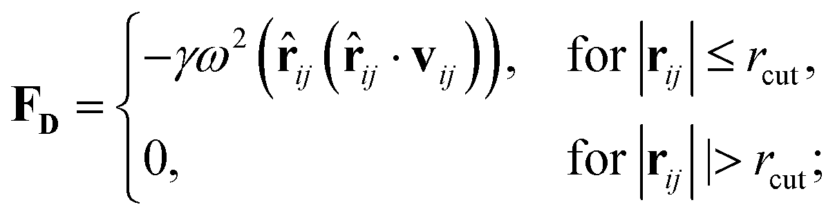 | (2) |
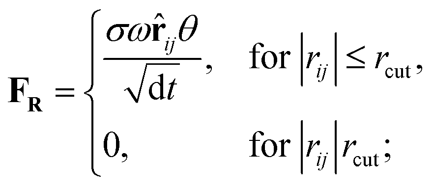 | (3) |
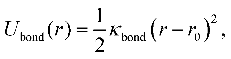
To provide a generic model for calamitic liquid crystals, (i.e. instead of a fully chemically tractable coarse graining scheme) we represent a liquid crystal mesogen by eight beads that are linearly bonded with harmonic bonds to maintain connectivity. Here,
 | (4) |
 | (5) |
Equations of motion were solved using the Velocity Verlet integration algorithm, using the DPD module of the DL_MESO50,51 program (DL_MESO_DPD) in the constant-NVT (canonical) ensemble. In each case, simulations were started from a random configuration (position and orientation) of 5000 molecules, which were initially equilibrated to an isotropic phase (T* = 2.0) and then cooled in a stepwise manner in increments of 0.1ΔT*/500000δt. We found that 500000 steps with a time step, δt, of  at each temperature was sufficient to ensure a well equilibrated phase in all cases studied. For some simulations we used larger system sizes of 50000 molecules to check the structure of smectic phases with a larger number of layers. The DPD parameter for noise amplitude was taken to be σ = 3.6710. The temperature is controlled by γ, such that the relationship between γ and σ is maintained, (σ2 = 2γT*). All simulations were performed at a particle site density ρ = 3.0(l−3). A mesogen showing a clear isotropic–nematic–smectic transition sequence was found for a model of eight linearly bonded beads, of a single type (type A), and with conservative force parameter aAA = 45.0ε. We define this as model 0 and this acts as a basis of comparison for later smectic phases.
Normally, for simulations of layered liquid crystals with relative small systems sizes, constant-NpT simulations are often needed in order to avoid the formation of layer structures that are incommensurate with the box dimensions. However, for the DPD method we employ here this is not necessary. Firstly, we use large system sizes, where we can check that the simulation box does not impose structure on the phase. Secondly, the simulation times used are extremely long relative to standard molecular dynamics models (in terms of both molecular diffusion and reorientation), so the director is quite easily able to rotate to a different orientation should a new phase start to form that is initially incommensurate with the periodic boundary conditions.
To favour antiparallel molecular interactions, two additional bead types were introduced (types B (blue) and C (red)). For all models the interaction parameters for the new beads were set to aAA = aAB = aAC = aBB = aCC = 45.0ε. However, the cross term aBC used to favour antiparallel molecular recognition, was set at a reduced value (with values of between 35.0ε and 5.0ε used below). Hence the magnitude of aBC controls the preference for antiparallel interactions, and the position of B and C groups within the molecule changes the location of the interaction (mimicking dipolar regions in different parts of the molecule).
Thirteen separate models were studied, as shown schematically in Fig. 1. As the strength of preferred B–C interactions is always relative to the maximum value of aij(45.0ε), we can define a “molecular recognition” variable arec = aij(max) − aBC to measure this, and classify the region between and including B and C in a molecule as the “molecular recognition” site.
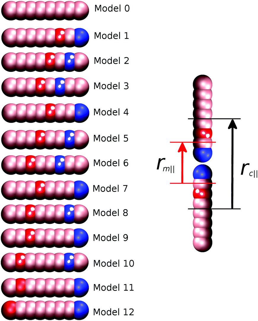 | ||
| Fig. 1 Left – Schematic diagram showing the thirteen DPD models studied in this work. Pink represents type A beads, blue type B and red type C. Beads are numbered sequentially from right to left. Right – Definition of parallel distances rc‖ and rm‖ for model 1. | ||
We note that in this simple model, molecular recognition is limited to interactions arising from just two sites per molecule, rather than from those arising from a large molecular segment. However, this is sufficient to enable favourable antiparallel configurations (in 8CB arising from π–π interactions in addition to antiparallel dipole interactions) without the use of computationally costly coulombic interactions.
The nematic order parameter for these systems was obtained by first defining a long-axis unit vector for each molecule, ui (from diagonalization of the molecular inertia tensor) followed by diagonalization of the order tensor
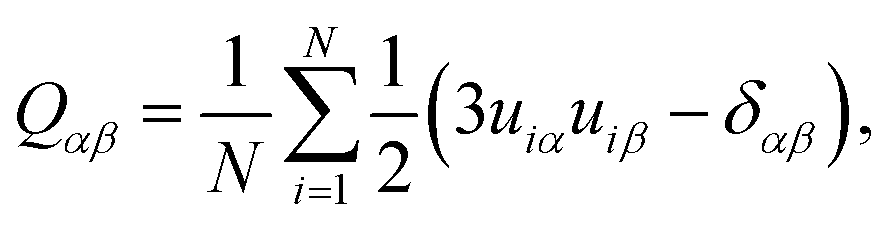 | (6) |
![[n with combining circumflex]](https://www.rsc.org/images/entities/b_char_006e_0302.gif) , given by the associated eigenvector. To further characterise mesophases, we introduce two pair correlation functions, g(rc‖) and g(rm‖), measured for intermolecular separations rc‖ and rm‖ along . Here,
, given by the associated eigenvector. To further characterise mesophases, we introduce two pair correlation functions, g(rc‖) and g(rm‖), measured for intermolecular separations rc‖ and rm‖ along . Here,| rm‖,c‖ = rij·. | (7) |
3 Results and discussion
3.1 Reference system – model 0 (SmA1 phase)
The reference model for this study, model 0, is provided by a mesogen of eight linearly-attached type A beads (Fig. 1). As expected, from previous work on hard sphere chains,52–54 hard and soft spherocylinders,11,55–59 and DPD chains,42 model 0 exhibits isotropic, nematic and smectic-A phases. On cooling from T* = 2.0 the isotropic–nematic transition was characterised by a discontinuous change in order parameter (see Fig. 2) at T* ≈ 1.15, and the onset of the smectic phase (at T* ≈ 0.9) was monitored through the growth of peaks in the radial distribution function resolved parallel to the director.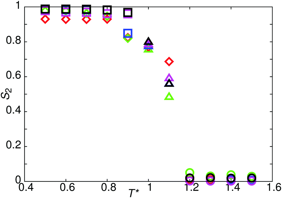 | ||
| Fig. 2 The temperature dependence of the nematic order parameter, S2, for model 0 (black symbols), and model 1 with arec = 40ε (red symbols), arec = 30ε (green symbols), arec = 20ε (blue symbols), arec = 10ε (pink symbols). Squares show a stable SmA1 phase, diamonds show a stable SmAd phase, triangles show a stable nematic phase and circles show a stable isotropic phase. | ||
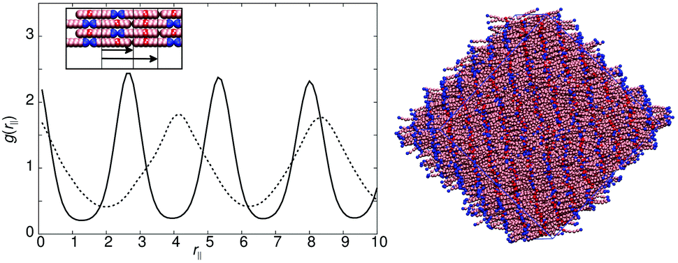
Fig. 3 shows the parallel pair distribution functions g(rc‖), from which a single layer spacing of d = 4.15l, is clearly observable. At low temperatures (T* = 0.8) the mean bond length is equal to 0.52l. Hence d corresponds to approximately one molecular length and the phase is a standard monolayer smectic A phase (SmA1).
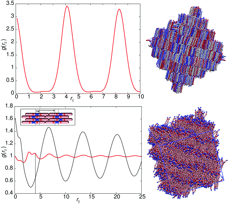 | ||
| Fig. 3 Top left: g(rc‖) for the smectic-A phase of model 0 at T* = 1.1. Top right: A simulation snapshot showing the structure of the smectic-A phase of model 0 at T* = 1.1. Bottom left: g(rm‖) (black) and g(rc‖) (red) for the smectic-Ad phase of model 1 at T* = 1.1, the solid vertical line indicates the expected spacing for a standard SmA1 phase. A schematic showing the expected packing of molecules is shown in the inset. Bottom right: A simulation snapshot showing the structure of the smectic-Ad phase of model 1 at T* = 1.1. | ||
Using the mean bond length (above) together with a mean width of 0.8l (minimum width = 0.5l), we obtain a molecular aspect ratio of ≈5.6:1 for our reference model (slightly less than this value if the flexibility of bond angles is taken into account). The low temperature model system is therefore slightly shorter than a 5:1 spherocylinder model.11
3.2 Interdigitated bilayers (SmAd phases): models 1, 4, 7 and 9
The models of this class all have a “molecular recognition” region located at one end of the molecule. Model 1 shows the presence of different smectic phases, and also shows a high sensitivity to the magnitude of arec. Fig. 2 shows the phase sequence obtained for four values of arec. For the highest value considered (arec = 40.0ε), a single transition is observed, from isotropic to smectic at T* = 1.1. The smectic A phase formed differs from that of model 0, as the layer spacing is considerably larger than one molecular length. This is evident from the pair correlation plots shown in Fig. 3. Here, the choice of pair correlation function is clearly important. g(rc‖) provides minimal information but g(rm‖) shows a repeat layer spacing of ≈1.5 molecular lengths. The centres of the layers are provided by the “molecular recognition” region, with the initial peak in g(rm‖) found at rm‖ = 0, together with a shoulder at 0.9l. From the snapshot, also shown in Fig. 3, pair-wise antiparallel correlation can be clearly observed within microphase segregated regions.The designation for the smectic phase is SmAd, and the model therefore mimics the smectic phase behaviour observed in longer chain homologues of the nCB (4-n-alkyl-4′-cyanobiphenyl) series, which show antiparallel dipole correlation arising from the large dipole associated with the terminal cyano group. This behaviour has been observed in atomistic simulation studies of 8CB (which has a layer spacing of 1.4 molecular lengths).20,31,32 However, the atomistic simulations are at the limit of what is currently computationally feasible. So for example, in ref. 32, pair distribution plots were only extendible to ∼30 Å, when the experimental layer spacing is 30.5 Å. Here, for simulations of 50000 molecules, we can resolve 4 layers in g(rm‖).
As in 8CB, the SmAd phase observed is not simply built from antiparallel dimers, in which every B site has two interacting C neighbours (in 2 dimensions). Such a phase would result in a shorter interlayer spacing (comparable to that of model 0) but with very tight (entropically unfavourable) packing of molecules from adjacent layers into spaces between dimers. Instead an alternative molecular packing is possible, as shown in the inset to Fig. 3, where half the C sites are able to interact with multiple B sites. This packing behaviour explains the additional 0.9l peak and the inter-layer spacing of 6.3l. It also leads to broader smectic layers than those seen in model 0.
Decreasing the molecular recognition parameter for model 1 to arec = 30.0ε, weakens the antiparallel association, resulting in subtly different phase behaviour. On cooling from the isotropic phase, a stable nematic phase is formed at T* = 1.1, prior to the formation of a SmAd phase. The local packing differs from that of a standard nematic, in that short range positional order is clearly detectable in g(rm‖), as shown in Fig. 4. We attribute the local positional order to transient antiparallel association, in agreement with the pre-transitional behaviour as noted in dielectric studies of cyanobiphenyl nematics.60–63 As temperature is reduced (Fig. 4), the strength of antiparallel correlation increases, resulting in cybotactic domains of SmAd phase within the nematic. Further reduction in the molecular recognition parameter arec = 10.0ε results in a nematic phase (Fig. 2), with far weaker local antiparallel correlation. At this value of arec the long layer spacing of a SmAd phase is lost, replaced by a standard SmA1 phase (at T* < 0.9), as observed in model 0.
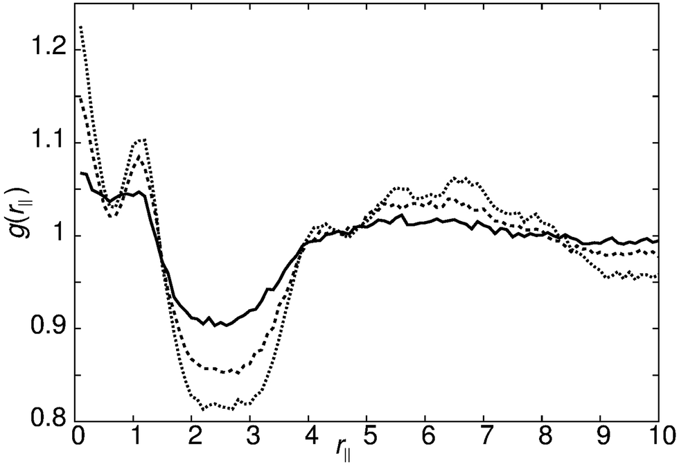 | ||
| Fig. 4 g(rm‖) for model 1 with arec = 30ε showing the growth of pretransitional fluctuations on cooling the nematic phase: T* = 1.1 (bold line), T* = 1.0 (dashed line) and T* = 0.9 (dotted line). | ||
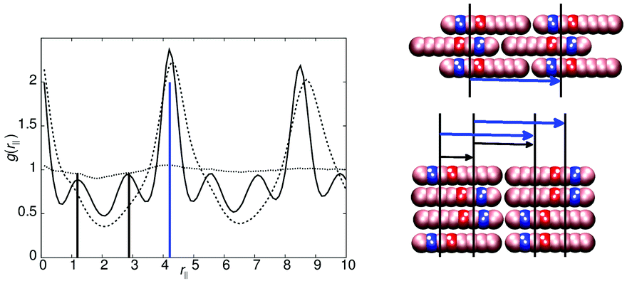
Model 4 (Fig. 1), has an increased distance between the antiparallel sites, leading to subtly different phase behaviour in comparison to model 1. For 10ε ≤ arec ≤ 40ε, on cooling from the isotropic phase, a nematic with local antiparallel correlation is formed with an onset temperature of T* = 1.1, and a smectic phase is formed at T* = 1.0. Both g(rm‖) and g(rc‖) show peaks at both half integral and integral molecular lengths. The shorter correlation length can be attributed to strong antiparallel packing causing intercalation of adjacent layers. The inset in Fig. 5 shows the local packing within the model, which supports each B interacting with C sites, and vice versa. However, the strict repeat distance for layers along the director is equivalent to two molecular lengths. The half molecular length displacement can occur in either a +ve or −ve direction along the director, and so packing of molecules into layers gives relatively sharp intensity peaks in g(rm‖) in comparison to the diffuse peaks observed for model 1. It is important to note that unlike 8CB and model 1, where only two sub-layers contribute to a single full layer; model 4 has three contributing sub-layers, as demonstrated by a comparison of the schematic insets for Fig. 3 and 5.
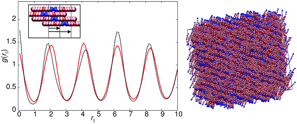 | ||
| Fig. 5 Left – g(rc‖) (red line) and g(rm‖) (black line) for model 4. Right – A simulation snapshot for model 4 with arec = 30ε at T* = 0.8. A schematic showing the expected packing of molecules is shown in the inset. | ||
The phase behaviour exhibited by model 4 is replicated by model 7 with the sole exception that for arec = 10.0ε the antiparallel correlation is sufficiently weak that it is lost completely in the smectic phase, with the formation of a SmA1 phase (as seen in model 0).
Model 9 exhibits two types of SmAd phase. For arec = 40.0ε and arec = 30.0ε, a strongly intercalated smectic phase is formed, comparable to that of model 4. However, for arec < 20.0ε a SmA1 phase is formed. The intercalated smectic phase has similarities with both models 1 and 4. Two peaks are seen in g(rm‖) at rm‖ = 2.7l and rm‖ = 5.2l, which correspond to the half layer and full layer peaks of model 4. These peaks are at slightly larger values of rm‖ than those observed in model 4, giving smectic layers with a width of 1.3 molecular lengths. The antiparallel packing is shown schematically in Fig. 6 and highlights that the packing arrangement adopted shares similarities with that of model 4, i.e. the B and C sites interact in an identical arrangement. However, the additional spacing between the two interaction sites subtly shifts the layer spacing to greater distances in a similar manner to model 1. Also the satellite peak, which occurred in model 1 at r = 0.9l, is displaced in model 9 towards the middle of the layer.
 | ||
| Fig. 6 Left: g(rm‖) for model 9 with arec = 30ε (bold line) and arec = 20ε (dotted line). Right: Simulation snapshot for arec = 30ε. A schematic showing the expected packing of molecules for the arec = 30ε model is shown in the inset. | ||
A summary of the phase behaviour of each of these models is given in Table 1.
| Model number | a rec/ε | Mesophases | T NI | T SN | Smectic phase type | Main peaksa in g(rm‖)/molecular length |
|---|---|---|---|---|---|---|
| a Here, the main peaks in g(rm‖)/are measured for distances as defined in Fig. 1. They therefore do not necessarily correspond to observable X-ray peaks, given the anti-parallel orientation of some neighbouring molecules. | ||||||
| 0 | 0 | iso–nem–sm | 1.15 | 0.95 | SmA1 | 1 |
| 1 | 40 | iso–sm | 1.15 | SmAd | 1.5 | |
| 1 | 30 | iso–nem–sm | 1.15 | 0.95 | SmAd | 1.5 |
| 1 | 20–10 | iso–nem–sm | 1.15 | 0.95 | SmA1 | 1 |
| 2 | 40–10 | iso–nem–sm–sm | 1.05 | 0.95 | SmA1 | 1 |
| 3 | 40–10 | iso–nem–sm | 1.15 | 1.05 | SmA1mic | 1 |
| 4 | 40–10 | iso–nem–sm | 1.15 | 1.05 | SmA2 | 1, 0.5 |
| 5 | 40–10 | iso–sm–sm | 1.05 | SmA1 | 1 | |
| 5 | 30–10 | iso–nem–sm–sm | 1.15 | 0.95 | SmA1 | 1 |
| 6 | 40–30 | iso–sm | 1.05 | SmA1mic | 1 | |
| 6 | 20–10 | iso–nem–sm | 1.05 | 0.95 | SmA1mic | 1 |
| 7 | 40–20 | iso–nem–sm | 1.15 | 0.95 | SmA2 | 1, 0.5 |
| 7 | 10 | iso–nem–sm | 1.15 | 0.85 | SmA1 | 1, 0.5 |
| 8 | 40 | iso–nem–sm | 1.15 | 0.95 | SmA1 | 1, 0.5 |
| 8 | 30–10 | iso–nem–sm | 1.15 | 0.95 | SmA1 | 1 |
| 9 | 40–30 | iso–sm | 1.15 | SmAd | 1.3, 0.7 | |
| 9 | 30–10 | iso–nem–sm | 1.15 | 0.95 | SmAd | 1.3, 0.7 |
| 9 | 20–10 | iso–nem–sm | 1.15 | 0.95 | SmA1 | 1 |
| 10 | 40–30 | iso–sm | 1.05 | SmA1mic | 1 | |
| 10 | 20–10 | iso–sm–nem | 1.15 | 0.95 | SmA1mic | 1 |
| 11 | 40–10 | iso–nem–sm | 1.15 | 0.95 | SmA1 | 1 |
| 12 | 40–10 | iso–sm | 1.55 | SmA1mic | 1 | |
3.3 SmA1 phases with microphase separation and in-layer antiparallel ordering: models 3, 6, 10, 11 and 12
Models 3, 6, 10, 11 and 12 all follow very similar phase behaviour. In all these models SmA1 phases are formed with a layer spacing of approximately one molecular length. Each system shows strong antiparallel ordering of molecules within the layer, and microphase separation into separate domains. Model 6 exhibits representative behaviour for this class of molecules. For arec = 40.0ε and arec = 30.0ε a single isotropic to SmA1 (T* = 1.0) transition is observed upon cooling, with sharp peaks in g(rm‖) indicating that molecules are “strongly bound” to smectic layers and more restricted in their motion parallel to the director. This arises because of strong in-layer antiparallel correlation, which leads to five microphase separated regions A–BC–A–BC–A. This ordering occurs naturally when the molecules sit exactly side-by-side and head-to-tail (see the snapshot in Fig. 7). As the strength of the interaction between the two recognition sites is reduced (arec = 20.0ε) a nematic phase (T* ∼ 1.05) is observable, with some (weak) positional order shown in g(rm‖), prior to smectic phase formation (T* ∼ 0.95).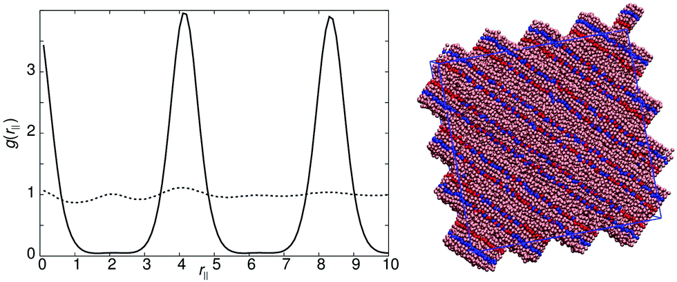 | ||
| Fig. 7 Left: g(rm‖) for model 6 with arec = 20ε, smectic phase at T* = 0.9l (bold line), nematic phase at T* = 1.0l (dotted line). Right: A simulation snapshot of the smectic phase for model 6. | ||
Model 10 behaves in an almost identical way to model 6, but with the position of the microphase separated domains shifted slightly. Model 12 behaves in a similar way, but with the positions of the B and C sites at the end of the molecule providing an additional inter-layer interaction. This leads to an exceptionally stable smectic A1 phase (stable up to T* ∼ 1.55), with no nematic phase observable at any temperatures for 10ε ≤ arec ≤ 40ε.
Models 3 and 11 differ slightly from the others in this section because the B and C sites are not equidistant from the centre of the molecule. This loss of symmetry, causes the smectic layers to be less strongly ordered (relative to models 6 and 12 respectively), reducing the thermal stability of the SmA1 phase relative to the nematic (see Table 1).
3.4 Complex SmA1 phases without microphase separation: models 2, 5, 8
The final type of phase behaviour is covered by models 2, 5 and 8. Here, complex SmA1 phases are formed with a layer spacing equivalent to one molecule. All these models form a standard SmA1 without microphase separation. In addition, for higher values of arec the models also exhibit a second smectic: in this case a microphase-separated intercalated smectic A phase, which retains a single layer repeat distance.The two smectic phases are easily observed in model 2 (with arec = 40ε), which exhibits a smectic to smectic phase transition at T* ≈ 0.85. The change in structure of the smectic is shown in g(rm‖) plots (Fig. 8), where at the phase transition additional peaks appear. In the schematic diagram (right of Fig. 8) we show how the additional correlations, corresponding to these peaks, arise from the local packing arrangement of molecules. In the case of the lower temperature phase, there is no specific preference for an antiparallel ordering of neighbours; instead, additional correlations arise from both parallel and antiparallel neighbours in equal measure.
 | ||
| Fig. 8 Left: g(rm‖) for model 2 with arec = 40ε, T* = 1.0l (dotted), T* = 0.9l (dashed), T* = 0.8l (bold). Right: Schematic showing the two packing arrangements, with indication of the expected g(rm‖) peaks. The vertical colour coded lines on the g(rm‖) functions indicate the expected location and intensity of the satellite (black) and full layer (blue) peaks. | ||
In the high-temperature intercalated smectic phase, the B and C sites do give rise to antiparallel ordering (see the top schematic diagram in Fig. 8), generating diffuse smectic layers. Here, however the average spacing remains equal to one molecular length. This complex layer structure is entropically favoured; hence the transition to a more conventional SmA1 phase as temperature is reduced.
The phase behaviour of model 5 is very similar to model 2 with small differences in transition temperatures and nematic stability. However, the behaviour of model 8 is subtly different. For arec = 40.0ε, isotropic–nematic (T* = 1.0)–smectic (T* = 0.9) transitions are seen, with the smectic phase exhibiting intercalated layers as observed in model 4. Here, the g(rm‖) function shows peaks corresponding to a half molecular length and a full molecular length (similar to model 4). The nematic phase that forms is very sensitive to arec. For arec ≥ 30ε, clear cybotactic domains are formed, which are ferroelectric in nature (see left hand side of the inset in Fig. 9). At lower values of arec cybotactic domains remain but the domains are of SmA1 character and are not ferroelectric (see right hand side of the inset in Fig. 9). The differences in the cybotactic domains show up as differences in the g(rm‖) plots in Fig. 9, noting that the peak intensities are much smaller than seen in smectic phases.
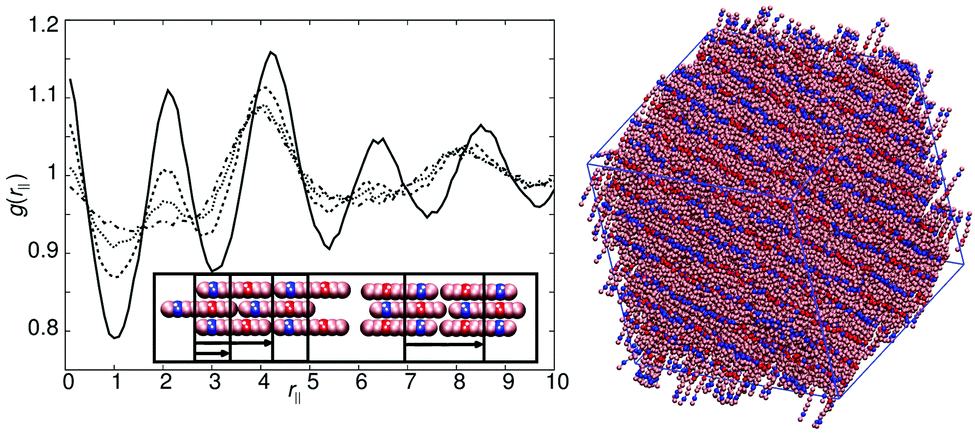 | ||
| Fig. 9 Left: g(rm‖) for the nematic phase of model 8 (T* = 1.0) with arec = 40ε (bold line), arec = 30ε (dashed line), arec = 20ε (dotted line) and arec = 10ε (dot-dashed line). The inset shows schematically the proposed two local smectic packing arrangements within the nematic phase that give rise to the peaks in g(rm‖). Right: A simulation snapshot of the smectic phase of model 8 for arec = 40ε at T* = 0.9. | ||
4 Conclusions
We present a simple DPD model, which can be used to represent calamitic mesogens. The model allows for antiparallel association that occurs naturally in a wide range of mesogens with terminal dipoles, including the 4-n-alkyl-4′-cyanobiphenyl series. In particular the model allows for the simulation of SmAd phases in which the layer spacing is intermediate between monolayer and bilayer, with the stabilization of intermediate layer spacings controlled by the strength of antiparallel association. The phase sequences are easily controlled by a single parameter, arec, which controls the strength of antiparallel association relative to kT. The model also allows for a range of other smectics: including SmA1 phases exhibiting microphase separation within layers (and hence very stable smectics); and smectic A structures in which we see an overall repeat structure of two molecular lengths but with repeat distances in g(rm‖) of approximately half a molecular length. These are all obtainable by subtle changes in the position of the “molecular recognition” sites within the molecule.The model also demonstrates the formation of cybotactic nematics in which pretransitional smectic fluctuations occur. For different models we identified three distinct types of cybotactic domains:
• normal SmA1 regions,
• SmA regions with molecules showing strong antiparallel correlation,
• ferroelectric smectic regions.
As expected, cybotactic domains grow as the system moves closer to the smectic–nematic phase transition.
Recently, there has been considerable controversy arising from the role (or otherwise) of cybotactic domains within the nematic phase. In particular, for some bent-core nematics these domains appear to be very extensive and different domain structures are possible;64 and it has been suggested that cybotactic domains may account for the NMR biaxiality observed in nematic phases of some mesogens.65 This current work suggests that simple DPD models can represent the twin features of molecular shape and specific pair-wise interactions responsible for cybotactic domain formation. Work applying these types of models to bent-core mesogens is currently under way in our laboratory.
References
- V. Borshch, Y.-K. Kim, J. Xiang, M. Gao, A. Jákli, V. P. Panov, J. K. Vij, C. T. Imrie, M. G. Tamba, G. H. Mehl and O. D. Lavrentovich, Nat. Commun., 2013, 4, 2635 CrossRef CAS PubMed.
- D. Demus, J. W. Goodby, G. W. Gray, H. W. Spiess and V. Vill, Handbook of Liquid Crystals, Low Molecular Weight Liquid Crystals I: Calamitic Liquid Crystals, John Wiley & Sons, 2011 Search PubMed.
- I. Sage, Liq. Cryst., 2011, 38, 1551–1561 CrossRef CAS.
- H. Coles and S. Morris, Nat. Photonics, 2010, 4, 676–685 CrossRef CAS.
- R. J. Bushby and K. Kawata, Liq. Cryst., 2011, 38, 1415–1426 CrossRef CAS.
- J. W. Goodby, Liq. Cryst., 2011, 38, 1363–1387 CrossRef CAS.
- J. Beeckman, K. Neyts and P. J. M. Vanbrabant, Opt. Eng., 2011, 50, 081202 CrossRef.
- M. R. Wilson, Chem. Soc. Rev., 1881, 2007, 36 Search PubMed.
- M. R. Wilson, Int. Rev. Phys. Chem., 2005, 24, 421–455 CrossRef CAS.
- P. Bolhuis and D. Frenkel, J. Chem. Phys., 1997, 106, 666–687 CrossRef CAS.
- S. C. McGrother, D. C. Williamson and G. Jackson, J. Chem. Phys., 1996, 104, 6755–6771 CrossRef CAS.
- J. A. C. Veerman and D. Frenkel, Phys. Rev. A: At., Mol., Opt. Phys., 1992, 45, 5632 CrossRef.
- J. G. Gay and B. J. Berne, J. Chem. Phys., 1981, 74, 3316 CrossRef CAS.
- M. A. Bates and G. R. Luckhurst, Structure and Bonding: Liquid Crystals, Springer-Verlag, Heidelberg, 1999, vol. 94 Search PubMed.
- R. Berardi, C. Fava and C. Zannoni, Chem. Phys. Lett., 1995, 236, 462–468 CrossRef CAS.
- A. Humpert and M. P. Allen, Mol. Phys., 2015, 113, 2680–2692 CrossRef CAS.
- M. P. Allen, M. A. Warren, M. R. Wilson, A. Sauron and W. Smith, J. Chem. Phys., 1996, 105, 2850–2858 CrossRef CAS.
- A. Cuetos, J. M. Ilnytskyi and M. R. Wilson, Mol. Phys., 2002, 100, 3839–3845 CrossRef CAS.
- N. J. Boyd and M. R. Wilson, Phys. Chem. Chem. Phys., 2015, 17, 24851–24865 RSC.
- M. F. Palermo, A. Pizzirusso, L. Muccioli and C. Zannoni, J. Chem. Phys., 2013, 138, 204901 CrossRef PubMed.
- G. Tiberio, L. Muccioli, R. Berardi and C. Zannoni, ChemPhysChem, 2009, 10, 125–136 CrossRef CAS PubMed.
- G. W. Gray, Thermotropic Liquid Crystals, Wiley, New York, 1987 Search PubMed.
- G. W. Gray and J. W. Goodby, Smectic Liquid Crystals, Leonard Hik Glasgow, 1984 Search PubMed.
- T. Kato, J. M. J. Frechet, P. G. Wilson, T. Saito, T. Uryu, A. Fujishima, C. Jin and F. Kaneuchi, Chem. Mater., 1993, 5, 1094–1100 CrossRef CAS.
- N. V. Madhusudana, Liq. Cryst., 2015, 42, 840–863 CAS.
- M. G. Lafouresse, M. B. Sied, H. Allouchi, D. O. López, J. Salud and J. L. Tamarit, Chem. Phys. Lett., 2003, 376, 188–193 CrossRef CAS.
- T. A. K. Lobko, O. D. Lavrentovich and S. Kumar, Mol. Cryst. Liq. Cryst., 1997, 304, 463–469 CrossRef.
- A. J. Leadbetter, J. L. A. Durrant and M. Rugman, Mol. Cryst. Liq. Cryst., 1976, 34, 231–235 CrossRef.
- J. E. Lydon and C. J. Coakley, J. Phys., Colloq., 1975, 36, C1-45–C1-48 Search PubMed.
- A. J. Leadbetter, R. M. Richardson and C. N. Colling, J. Phys., Colloq., 1975, 36, C1-37–C1-43 CrossRef.
- Y. Lansac, M. A. Glaser and N. A. Clark, Phys. Rev. E: Stat., Nonlinear, Soft Matter Phys., 2001, 64, 051703 CrossRef CAS PubMed.
- F. Chami, M. R. Wilson and V. S. Oganesyan, Soft Matter, 2012, 8, 6823–6833 RSC.
- P. G. de Gennes and J. Prost, The Physics of Liquid Crystals, Oxford University Press, 2nd edn, 1993, ch. 10 Search PubMed.
- R. D. Groot, T. J. Madden and D. J. Tildesley, J. Chem. Phys., 1999, 110, 9739–9749 CrossRef CAS.
- A. A. Gavrilov, Y. V. Kudryavtsev and A. V. Chertovich, J. Chem. Phys., 2013, 139, 224901 CrossRef PubMed.
- L. He, Z. Chen, R. Zhang, L. Zhang and Z. Jiang, J. Chem. Phys., 2013, 138, 094907 CrossRef PubMed.
- E. S. Boek, P. V. Coveney, H. N. W. Lekkerkerker and P. van der Schoot, Phys. Rev. E: Stat., Nonlinear, Soft Matter Phys., 1997, 55, 3124–3133 CrossRef CAS.
- S. Yamamoto, Y. Maruyama and S.-A. Hyodo, J. Chem. Phys., 2002, 116, 5842–5849 CrossRef CAS.
- J. C. Shillcock and R. Lipowsky, J. Chem. Phys., 2002, 117, 5048–5061 CrossRef CAS.
- H. Xu, Q. Zhang, H. Zhang, B. Zhang and C. Yin, J. Theor. Comput. Chem., 2012, 12, 1250111 CrossRef.
- X. Chen, F. Tian, X. Zhang and W. Wang, Soft Matter, 2013, 9, 7592–7600 RSC.
- A. Al Sunaidi, W. K. Den Otter and J. H. R. Clarke, Philos. Trans. R. Soc., A, 2004, 362, 1773–1781 CrossRef CAS PubMed.
- A. Al Sunaidi, W. K. Den Otter and J. H. R. Clarke, J. Chem. Phys., 2013, 138, 154904 CrossRef CAS PubMed.
- M. A. Bates and M. Walker, Phys. Chem. Chem. Phys., 2009, 11, 1893–1900 RSC.
- M. Bates and M. Walker, Soft Matter, 2009, 5, 346–353 RSC.
- M. A. Bates and M. Walker, Mol. Cryst. Liq. Cryst., 2010, 525, 204–211 CrossRef CAS.
- M. A. Bates and M. Walker, Liq. Cryst., 2011, 38, 1749–1757 CrossRef CAS.
- M. Walker, A. J. Masters and M. R. Wilson, Phys. Chem. Chem. Phys., 2014, 16, 23074–23081 RSC.
- R. D. Groot and P. B. Warren, J. Chem. Phys., 1997, 107, 4423–4435 CrossRef CAS.
- M. A. Seaton, R. L. Anderson, S. Metz and W. Smith, Mol. Simul., 2013, 39, 796–821 CrossRef CAS.
- DL_MESO is a mesoscale simulation package written by R. Qin, W. Smith and M. A. Seaton and has been obtained from STFC's Daresbury Laboratory via the website http://www.ccp5.ac.uk/DL_MESO.
- M. R. Wilson and M. P. Allen, Mol. Phys., 1993, 80, 277–295 CrossRef CAS.
- M. R. Wilson, Mol. Phys., 1994, 81, 675–690 CrossRef CAS.
- D. C. Williamson and G. Jackson, J. Chem. Phys., 1998, 108, 10294–10302 CrossRef CAS.
- D. Frenkel, H. N. W. Lekkerkerker and A. Stroobants, Nature, 1988, 332, 822–823 CrossRef CAS.
- J. A. C. Veerman and D. Frenkel, Phys. Rev. A: At., Mol., Opt. Phys., 1990, 41, 3237 CrossRef CAS.
- D. J. Earl, J. Ilnytskyi and M. R. Wilson, Mol. Phys., 2001, 99, 1719–1726 CrossRef CAS.
- Z. E. Hughes, L. M. Stimson, H. Slim, J. S. Lintuvuori, J. M. Ilnytskyi and M. R. Wilson, Comput. Phys. Commun., 2008, 178, 724–731 CrossRef CAS.
- J. S. Lintuvuori and M. R. Wilson, J. Chem. Phys., 2008, 128, 044906 CrossRef PubMed.
- M. J. Bradshaw and E. P. Raynes, Mol. Cryst. Liq. Cryst., 1981, 72, 73–78 CrossRef CAS.
- J. Thoen and G. Menu, Mol. Cryst. Liq. Cryst., 1983, 97, 163–176 CrossRef CAS.
- M. Schadt, J. Chem. Phys., 1972, 56, 1494–1497 CrossRef CAS.
- N. Madhusudana and S. Chandrasekhar, Pramana, Suppl., n1, 1975, 1, 57–68 Search PubMed.
- C. Tschierske and D. J. Photinos, J. Mater. Chem., 2010, 20, 4263–4294 RSC.
- O. Francescangeli and E. T. Samulski, Soft Matter, 2010, 6, 2413–2420 RSC.
| This journal is © The Royal Society of Chemistry 2016 |