A single nucleotide resolution model for large-scale simulations of double stranded DNA

Abstract

The computational modelling of DNA is becoming crucial in light of new advances in DNA nano-technology, single-molecule experiments and in vivo DNA tampering. Here we present a mesoscopic model for double stranded DNA (dsDNA) at the single nucleotide level which retains the characteristic helical structure, while being able to simulate large molecules – up to a million base pairs – for time-scales which are relevant to physiological processes. This is made possible by an efficient and highly-parallelised implementation of the model which we discuss here. The model captures the main characteristics of DNA, such as the different persistence lengths for double and single strands, pitch, torsional rigidity and the presence of major and minor grooves. The model constitutes a starting point for the future implementation of further features, such as sequence specificity and electrostatic repulsion. We show that the behaviour of the presented model compares favourably with single molecule experiments where dsDNA is manipulated by external forces or torques. We finally present some results on the kinetics of denaturation of linear DNA and supercoiling of closed dsDNA molecules.

---

1 Introduction

Since the discovery of the structure of the deoxyribonucleic acid (DNA),^1–3 the geometry of the double-helix and its topological implications have engaged and fascinated the scientific community.^4,5 It is becoming more and more evident that not only is the genetic information encoded in the DNA sequence of primary importance, but also that changes in its three-dimensional structure can alter crucial biological functions, such as gene expression and replication.^6–10 At the same time, the rapid improvement of techniques using DNA functionalised colloids,^11,12 DNA-origami¹³ and, more generally, supra-molecular DNA assembly¹⁴ is setting new standards for DNA-based nano-technology. This has far-reaching applications, ranging from materials science (to create new DNA-based and possibly biomimetic materials), to medicine (to be used in, e.g., gene-therapy and drug delivery). In light of this, the formulation of accurate theoretical and computational models that can efficiently capture the behaviour of DNA, either in vivo or in vitro, is of great importance in order to understand a number of outstanding biological problems, and also to assist the advance of DNA-based nanotechnology.

Several fully atomistic models for double-stranded (ds) DNA are available in the literature.^15–17 While these give an accurate description of the dynamics of DNA molecules and their interaction with single proteins, the complexity of the all-atom approach places severe limits on the size (up to about a hundred base-pairs) and time scales (of the order of μs) which can be probed.¹⁸ Coarse-graining, where large collections of atoms or molecules are represented by single units, allows larger systems to be simulated for longer at the expense of molecular detail. One of the most challenging aspects in designing a computational model is to retain the key microscopic details necessary to answer a given question while “trimming” the rest. At the large scale limit, entire eukaryotic chromosomes can be modelled using simple bead-and-spring polymer models,^7,19 where each monomer can represent up to 3000 base-pairs (bp) and the simulated time can reach time-scales spanning minutes¹⁹ or even several hours;²⁰ similar chains of beads can also be used to model naked DNA, though clearly such an approach neglects microscopic details such as the base-pair specificity or the double-stranded structure. While in some cases these models can still capture the essential physics,²¹ in others they are only a crude approximation of the real systems. Several successful mesoscopic models have recently been proposed which aim at bridging the gap between the “all-atom” and “bead-spring” limits.^22–25 Nevertheless, a coarse grained model able to retain the necessary physical microscopic details while allowing simulations of the several tens or hundreds of kilo-base pairs (kbp) that would be needed to address many biologically relevant questions, is still currently needed.

Examples of biological processes for which such a mesoscopic approach would be highly valuable can be classified in two broad categories: processes where DNA is mechanically manipulated by enzymatic machines (for example during replication or transcription which require opening of the double-helical structure), or processes where interactions between DNA and proteins depend more subtly on the topological and geometrical properties of the double-helix. An example of the latter class of problems is the so-called “linking number paradox”, where it has been observed that the unbinding of DNA from a nucleosome releases only one unit of linking number, rather than the 1.7 units of writhe which were stored;^26,27 the resolution of the paradox is that the nucleosome also stores some twist (the terms twist and writhe are explained below). To complicate the picture even more, there are several proteins which operate to alter the DNA topology, whose collective actions may sometimes trigger complex feedback mechanisms that are crucial for biological functions.^28,29 For a model to be applicable to such problems, it must possess both a good accuracy in mimicking the geometry of the double-helix, and the ability to consider long molecules on which many proteins may act simultaneously, so that cooperative effects can be investigated.

Motivated by this goal, in this paper we introduce a single nucleotide resolution coarse-grained model for dsDNA which retains several biologically-relevant DNA features, while being capable of delivering large-scale simulations. The model is implemented in the LAMMPS molecular dynamics engine³⁰ which allows us to comfortably study molecules on the order of thousands of bp (kbp). Because the code is fully parallel and highly scalable, it is portable to supercomputers to reach the length and time scales needed for some of the biological applications just mentioned. The scope of this work is to present the construction of the model, starting from the known geometry of DNA⁴ (Section 2), and to discuss the validation of its main physical features, i.e. helical pitch, persistence length and torsional rigidity (Section 3). These properties are traditionally addressed via single-molecule experiments^31,32in vitro, and we here provide an indirect validation via simulated single-molecule experiments, obtaining a remarkably good agreement with the experimentally observed values (Section 4). Finally, we present an application of this model to the dynamics of DNA denaturation, and discuss further future applications. These range from the study of DNA denaturation to that of supercoil dynamics in the presence of topological proteins (Section 6). The flexibility of the model and the scalability provided by the LAMMPS engine means it provides a solid framework on which to base further studies of the topological properties of DNA and DNA–protein interactions.

2 The model

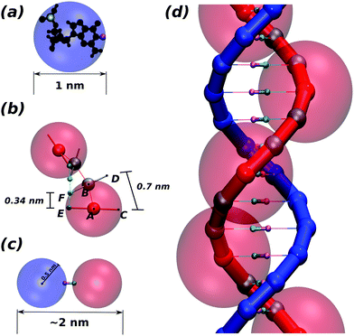
We start by considering a complex made of two spherical monomers (see Fig. 1(a)), one of which represents the sugar-phosphate backbone of the DNA (this is referred to as a “bead” hereafter, and shown in blue), while the other represents the nitrogenous base (“patch” hereafter, shown in pink), and is placed at a distance of 0.5 nm from the bead centre. Beads have an excluded volume so that they cannot overlap, whereas patches have no associated excluded volume. In order to see the resolution of the system, a nucleotide structure lying inside the bead is shown in black in Fig. 1(a).

Fig. 1 (a) The level of coarse-graining of the model is here summarised by encapsulating the atoms forming one nucleotide into one bead-patch complex. The small yellow sphere represents the position of the phosphate with respect to the complex, while the pink sphere denotes the position of the hydrogen bond between bases. The blue sphere approximates the excluded volume of the nucleotide. (b) This panel shows the main interaction sites between consecutive beads in the same strand. The equilibrium distance between patches (E–F) is set to 0.34 nm while the one between beads centres (A–B) to 0.46 nm. This leads to an equilibrium distance of 0.7 nm between the external edge of the backbone (C–D). These distances are set so that the correct pitch of 10 bp is recovered. (c) Two nucleotides are bonded via a breakable harmonic spring. Their distance is set so that the full chain thickness is around 2 nm, as that of B-DNA. (d) Representation of the double-stranded DNA model. The red chain also shows the beads which interact sterically (solid red) as well as the phantom beads (solid grey). The faded red spheres represent the steric interaction volume of the red beads. Neither the interacting beads nor the ghost beads along the blue chain are shown to ease visualisation.

Depending on the relevant features of the system to be modelled, a second patch representing the phosphate group may also be included explicitly to more accurately represent the DNA steric hindrance. When this second patch is not included, we imply that the phosphate is sitting 0.5 nm from the bead centre but slightly away from the antipodal point to the patch, marked in yellow in Fig. 1(a) for clarity.

Each bead-patch complex thus represents a single nucleotide, and acts as a rigid body; we connect a chain of these bodies via FENE bonds of length d_bp = 0.46 nm between the beads to represent one strand of DNA. We set the distance between two consecutive patches along the strand (E–F in Fig. 1(b)) at 0.34 nm by means of a Morse potential; the difference between the lengths A–B and E–F implies that the distance between the implicit phosphates at the external edge of the beads (C–D in Fig. 1(b)) is d_ph = 0.7 nm. The ratio between d_bp and d_ph is well known to crucially regulate the correct pitch of the chain⁴ (for details about the potentials used see Appendix A).

Nucleotides belonging to different strands are bonded together via breakable harmonic springs acting between two patches and representing hydrogen bonds (see Fig. 1(c)). The equilibrium bond distance is set to zero; if the extent of the bond increases beyond a critical value r_c = 0.3 nm, the bond breaks, modelling the denaturation of the chain.

While the pitch of the chain is set by the ratio of the base pairing distance and the distance between successive phosphate groups on a DNA strand, the right-handedness is imposed using a dihedral potential between the quadruplets of monomers forming two consecutive nucleotides (A, E, F and B in Fig. 1(b)). This potential regulates the angle between the planes A–E–F and E–F–B. The minimum of this potential is set equal to 36°, so as to match the geometry of a regular dsDNA helix.

In order to limit the splay of consecutive nucleotides (also called “roll”⁴) we used a stiff harmonic potential so as to keep the angle between particles E, F and B (two patches and one bead) at 90° (Fig. 1(b)). This interaction imposes the planarity between consecutive bases in the same strand. Finally, the last ingredient of this model is a Kratky–Porod potential regulating the angle between three consecutive patches along one strand. This allows us to finely regulate the chain stiffness.

The excluded volume around each bead depicted in Fig. 1(d) (faded red spheres) has diameter 1 nm. Since we use spherical beads rather than asymmetrically shaped ones (this is important for the speed of the algorithm), the geometry of the double-strand depicted in Fig. 1(b and d) would involve a large degree of overlapping which would lead to a large steric repulsion. To avoid this we consider two types of beads in each strand: sterically interacting beads (shown as small solid red spheres for one strand in Fig. 1(d)) are intercalated by two ghost beads (depicted as small grey spheres) which do not interact sterically along the same strand but they do interact with all the beads on the complementary strand with an excluded volume of 0.5 nm. This choice ensures that only non-overlapping beads sterically interact with one another. In addition, this allows us to preserve the correct thickness of the chain (2 nm for B-DNA), to maintain the desired distance between contiguous nucleotides and avoid the strands crossing through one another. In Fig. 2 we show a typical equilibrated configuration using the presented model for a 1000 bp molecule.

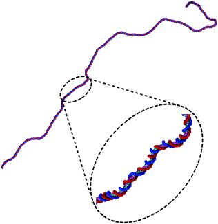Fig. 2 An example of an equilibrated configuration of a 1000 bp double-stranded DNA molecule, as simulated with the model presented in Section 1.

We should stress here that the model as presented in this section should be thought of as a simple, starting point, which is based on some crucial geometric constraints of double-stranded DNA. One of the main strength of the model is the ability to deliver large-scale simulations, which is achieved by using spherical monomers that interact via standard potentials. These are efficiently implemented in LAMMPS and ensure a highly scalable performance in large scale parallel simulations (see Appendix A for more details). From now on, we only show results for the model without the explicit presence of the phosphates unless otherwise noted. At the same time, there are several characteristics of dsDNA that the model (as presented up to now) does not include. Some notable examples are: (i) the distinction between minor and major groove; (ii) the description of electrostatic effects due to charges on the DNA, and to the variation of the density of counter-ions in solution (our parameters are tuned assuming room temperature and a physiological buffer, 0.15 M NaCl, see Appendix A); and (iii) the effect of sequence heterogeneity, or sequence specificity (in this simplest description, our dsDNA is viewed as a homopolymer). Such effects will be important, for instance, when one needs to more faithfully describe interactions between DNA and DNA-binding proteins. It is in principle possible to include these effects in a modular fashion in our framework, and in the Discussion (see also Appendix B) we describe how we can account for (i) in a simple way, and how (ii) and (iii) might be implemented in the future.

It is worth mentioning that in the current version of the model, hydrogen bonding is the only interaction responsible for holding the two DNA strands together. The rest of the potentials are defined independently for each strand. As a consequence, when the model was tested for single stranded DNA (ssDNA), and the persistence length was computed, its value (30 nm) was higher than expected from experiments³³ (≈1–2 nm). To model ssDNA and reproduce this dramatic change in flexibility, we set that, once the hydrogen bond keeping the two strands together breaks, both the dihedral and the Kratky–Porod potentials acting on each individual strand should be turned-off. In this way, we effectively take into account of the larger flexibility of single DNA strands and, in particular, we observe a persistence length of about 1 nm (see Section 5).

3 Parameterisation

Our model has several parameters which can be varied to control the pitch, bending and torsional properties of the simulated DNA molecule. Nonetheless, we are interested in modelling the B form of dsDNA, of which two main physical properties are: the persistence length l_p = 50 nm ≃ 150 bp, and the torsional rigidity C/k_BT ≃ 60–80 nm ≃ 177–235 bp.^34–36 Due to the interplay between the potentials presented in the previous section, there is no simple mapping between individual simulation parameters and the resulting physical properties; instead we obtain a simulated molecule with the correct values of l_p and C via a systematic tuning of the parameters. In this section we measure these properties from the microscopic positions of the beads in equilibrated DNA molecule configurations. Then in the following section, we use the parametrised force field to simulate single-molecule experiments, showing that the DNA molecules show the correct macroscopic response to mechanical manipulations.

3.1 Persistence length

The persistence length of dsDNA is a well-studied physical property that plays an important role in the wrapping of dsDNA around histone octamers to form the chromatin fibre, as well as in many other biological processes. In physical terms it gives a measure of the length-scale over which the direction of the chain is no longer correlated with itself. Following the description of an elastic rod by Moroz and Nelson³⁷ one can define the bending rigidity via the elastic energy functionalwhere l_p is the bending persistence length, s the arclength parameter and t(s) = dr/ds the tangent to the chain (at s) whose location in space is described by r(s). This quantity can also be readily measured by computing the tangent–tangent correlator:

〈t(s)·t(s′)〉 = e^{−|s−s′|/l_p}. (2)

In our model, we use the position of the patches to extract the centreline of the dsDNA molecule, where the tangent at the nth patch at position r(n) is t(n) ≡ (r(n + 1) − r(n))/|r(n + 1) − r(n)|. One can compute the tangent–tangent correlator along this curve and obtain the persistence length by extracting the exponent of the exponential decay. In order to avoid finite-size effects due to the presence of ends, we neglect the two terminal segments (∼5 bp at each end). The resulting curve (shown in Fig. 3) is adjusted by tuning the parameters of the model and until the exponential fit returns a persistence length of l_p ≃ 143 ± 7 bp, in agreement with the experimentally observed values.

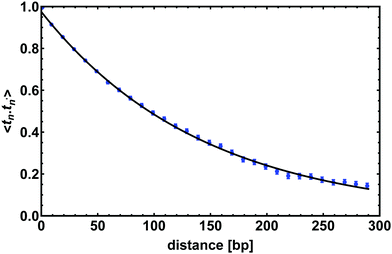Fig. 3 The tangent–tangent correlator 〈t(n)·t(n′)〉 computed for a chain 300 bp long; it shows an exponential decay as in eqn (2) with a correlation length l_p = 143 ± 7 bp. Points show correlations measured from the simulations (average over time), and the line shows a fit to eqn (2). Error bars give the standard error of the mean.

3.2 Torsional rigidity

The behaviour of DNA when twisted is regulated by its torsional rigidity. There are several well known examples in which this property is crucial for important biological processes, such as transcription and gene expression.^28,29 Furthermore, the high torsional stiffness of DNA molecules implies that, when placed under torsion, they preferentially bend, thereby creating writhe and plectonemes.⁴ In order to take this feature correctly into account, it is therefore crucial to accurately model the competition between bending and torsional rigidities.³⁶

Following Moroz and Nelson³⁷ once again, we first define the torsional stiffness of an elastic rod C via the elastic energy functional

where Ω₃(s) is the rate of rotation of a local reference frame along the curve around the tangent t(s), defined as in the previous section.

Analogous to the measurement for the bending persistence length via the tangent–tangent correlator, we here measure the torsional persistence length by computing the decorrelation of the twist angle. This correlator can be quantified by defining a local reference frame for each base pair, and tracking the rotation of the frames from one base pair to the next via their Euler angles. Each local frame is specified by the tangent vector t(n) as defined above, a normal vector f(n), defined as the projection of the vector connecting two beads in a base-pair onto the plane perpendicular to t(n), and a third vector v(n) = t(n) × f(n), perpendicular to both t(n) and f(n).

The Euler angles between the frames at n and n + 1 can be used to obtain the twist increment between those base-pairs, and the correlation function for the total twist between m consecutive base-pairs Ω(m) calculated. Since dsDNA has an equilibrium twist angle θ₀ = 36° per bp, we subtract this out, and calculate the correlation for the residual twist ΔΩ(m) = Ω(m) − mθ₀. It can be in fact shown³⁸ (see also Appendix C) that the average cosine of the residual total twist between any two reference frames separated by m bases exhibits an exponential decay as:

〈cos ΔΩ(m)〉 = e^−m/2C, (4)

where we define l_τ = 2C the characteristic torsional correlation length. We obtain 〈cos ΔΩ(m)〉 by simulating a 300 bp long dsDNA molecule and by averaging the value over time. The curve obtained is shown in Fig. 4 on top of which we show the fitted exponential. Again, we tune the parameters of the model so that the curve displays a characteristic decay length l_τ = 512 ± 18 bp ≃ 174 ± 6 nm, which is consistent with experimental estimates valid for the B-form of dsDNA.

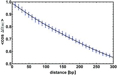Fig. 4 The average of the cosine of the total twist angle ΔΩ(m) is computed for a chain 300 bp long; in this figure we show the correlator to decay exponentially as in eqn (4) with a characteristic length l_τ = 512 ± 18 bp. Data points are obtained from simulations while the line is an exponential fit. Error bars give standard error of the mean.

4 Validation through single molecule experiments

Many cellular processes, such as replication and transcription, are carried out by proteins acting on single DNA segments. In light of this, recent years have seen an increasing interest in experimental techniques such as optical tweezers and atomic force microscopy, that can probe the response of DNA to external stresses (modelling the effect of DNA-binding enzymes) at the single-molecule level. In particular, the stretching and twisting behaviour of DNA under external forces and torques has been thoroughly investigated.^{31,34–36,39–41}

In this section we reproduce the conditions of two different experiments, in order to test the response of our model DNA to stretching and twisting. This also provides us with an independent method to evaluate its persistence length and torsional rigidity. In the following, we therefore keep the parameters of the model fixed at the values used in the previous section, and do not further tune them to achieve the experimentally known behaviours but simply validate the model as it is through its response to mechanical stress.

4.1 Response to stretching

The classic elastic response of DNA to an external stretching force F is known to be well described by the inextensible worm-like chain (WLC) for forces up to 10 pN. Using this framework, the force required to induce an end-to-end distance R_z = [r(L) − r(0)]·e_z for a chain of length L and persistence length l_p can be approximated by:^42,43where excluded volume effects are neglected (a good approximation when L is not much larger than l_p, as in our case). In order to test if our model can reproduce this result, we performed simulations in which a constant pulling force directed along e_z and acting on the last base pair of the dsDNA was applied, while the other end of the molecule was anchored at a surface (see Fig. 5).

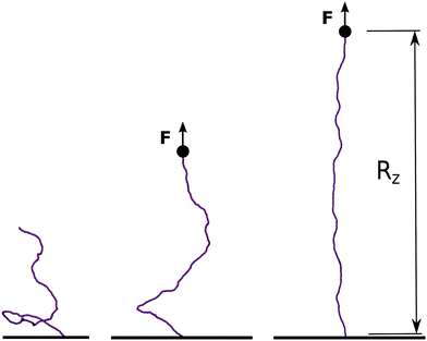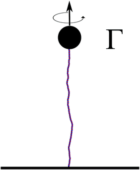
Fig. 5 In order to simulate single-molecule experiments the model for dsDNA is anchored to a surface at the bottom end while being stretched with a constant force F from the top end. We then monitor the end-to-end elongation along the z-direction, R_z, and report its equilibrium value for a given force in Fig. 6.

The force–extension curve³¹ measured for a chain 300 bp long is reported in the inset of Fig. 6 as data points, while the solid curve is the fit to eqn (5). The fitting results in values for both L and l_p, that we can compare with the values obtained in the previous sections and set by the parameters of our model. In particular for a 300 bp chain we obtain L = 100.3 ± 1.7 nm (which gives a bp step size of 0.33 ± 0.01 nm) and l_p = 47 ± 2 nm ≃ 140 ± 7 bp. In the previous section, we obtained a value for l_p of 49 nm. The results are therefore in good agreement with the calculation and the tuning of the persistence length performed in the previous section.

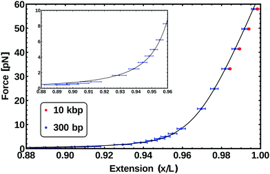Fig. 6 Force–extension curve from the simulation (data points) of two different length chains: 300 bp (blue) and 10 kbp (red). The inset data (low force regime) is fitted by the function in eqn (5) (solid line) and the data above 10 pN is fitted with eqn (6). For the WLC the free parameters for the fitting are the total polymer length L and the persistence length l_p, both of which are in agreement with the fixed parameters of the model (see text). For the EWL in addition to the previous parameters the stretching modulus S is found.

When the applied force is greater than 10 pN the existence of a finite stretching modulus (S) has to be taken into account. The Extensible WLC (EWLC) has proven to be the most adequate model to describe this particular case.³³ This model assumes that the contour length of the molecule increases linearly with the applied force,⁴⁴ and the following formula can be used between 5 and 50 pN:⁴⁵

The force–extension curve from the simulations of a 300 bp chain in this regime, corresponds to the data points above 10 pN shown in blue in Fig. 6. Fitting these points with eqn (6) gives L = 99.7 ± 0.5 nm, l_p = 60.2 ± 2 nm and S = 2086 ± 23 pN. This value of L is the one expected for a chain made by 300 bp. The value for the persistence length l_p is slightly bigger than the one observed in the WLC regime; on the other hand, this apparent increase of l_p is also observed in experiments.³³ Finally, the stretching modulus S is found to be twice the one expected for real dsDNA (∼1000 pN), although this difference should not be critical to the processes we are interested in the following.

We also performed simulations of a stretching experiment on a chain ten thousand base-pairs long (comparable to viral P4 DNA). The results for this case are reported as red data-points in Fig. 6. These measurements are in agreement with the behaviour of the 300 bp-long chain within error-bars, although they systematically show a slightly larger extension, possibly due to finite-size effects.

At forces of 65 pN or more, dsDNA changes its form dramatically³³ and it has been observed to stretch up to 70% beyond the canonical contour length shown by its B-form. This is not currently reproduced in our model and it would require a change in the structure of how the base-pairs are arranged and stacked together (i.e. the distance between base-pairs would no longer be 0.34 nm).

4.2 Response to twisting

The torsional stiffness of DNA can be calculated by computing the twist response of dsDNA to an imposed external torque, for instance applied by a magnetically controlled macroscopic bead^36,46 (see Fig. 7). For different magnitudes of the applied torque, |Γ|, we compute the superhelical density, σ. The level of supercoiling is determined by the linking number Lk, which is the number of times one DNA strand wraps round the other.

Fig. 7 The model DNA is anchored to a surface at the bottom end while being stretched with a constant force F, and a torque Γ is applied at the top end. We then monitor the linking number and report its equilibrium value for a given torque. With this information is possible to compute the superhelical density.

Since a dsDNA chain has a preferred equilibrium linking number Lk₀, the superhelical density may be defined as σ = (Lk − Lk₀)/Lk₀. The well-known White–Fuller theorem⁴⁷

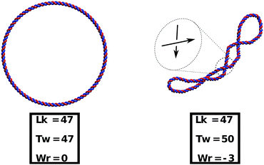
Lk = Tw + Wr, (7)

relates the linking number of the edges of a ribbon (Lk) to the twist (Tw), i.e. the extent of rotation of the two ribbon edges about the axis, and the writhe (Wr), i.e. the number of self-crossings of the ribbon centreline. Although the chain we use is not closed into a loop, and therefore it is not possible to formally define a linking between the strands, it is possible to compute the linking number between two “artificially” closed strands^48,49 which follow the paths of the DNA strands along the chain backbone and then join the respective ends far away from the molecule (see Appendix D). Furthermore, the molecule is kept straight (writhe-free) by applying a constant stretching force which ensures that the twist is very close to the computed linking number.

By measuring the deviation of twist ΔTw from the equilibrium value Tw₀ = N/p, i.e. the number of base-pairs divided by the pitch p = 10 bp, we can then readily obtain σ. With this information it is possible to map out the response curve of the molecule to an external torque. A feature of this is a linear regime for small |σ| which we recover (see Fig. 8). The torsional rigidity, C, can finally be calculated (in the limit of large stretching forces²⁵) as³⁷

where a₀ = 0.34 nm and θ₀ = 36° are respectively the double helical rise and the equilibrium twist angle across a base-pair step for a relaxed dsDNA molecule.

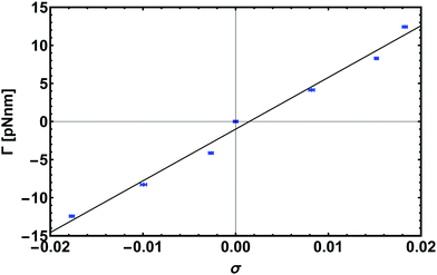Fig. 8 Response to torque experiment for a chain 600 bp long pulled with an external stretching force of 16 pN. Here we show the linear regime for small |σ| which gives the torsional rigidity C by a linear fit with eqn (8).

The data points shown in Fig. 8 are obtained from simulations of a 600 bp long chain anchored at a surface to one end, while the other end was pulled by a constant force of 16 pN and different applied torques, Γ = Γ·e_z. From the fit we get the value of torsional persistence length C ∼ 88 nm ≃ 260 bp in good agreement with experimental results.^50–52 One can finally use the relation between the torsional persistence length l_τ and the torsional stiffness C obtained from the twistable worm-like chain theory,³⁸ which gives l_τ = 2C ∼ 176 nm, very close to the measurement performed in the previous section (yielding l_τ = 174 ± 6 nm).

5 DNA denaturation and supercoiling

DNA denaturation is the separation and unwinding of the two strands, transforming a DNA duplex into two isolated and unbound single strands.⁵³ This process can be driven by heating a solution of dsDNA molecules, and a critical “melting” temperature T_m can be defined as the temperature at which 50% of a long dsDNA molecule is denatured. This critical temperature commonly depends on the genetic sequence, pH and salt concentration.^50,54,55 Localised, temporary, and dynamic denatured segments are often referred to as “bubbles”.

It is well known that local denaturation has several biological implications such as favouring transcription initiation, DNA repair or recombination,^28,56,57 and that the dynamics of these bubbles can be affected by torsional stress, which is itself often regulated by enzymes, such as RNA polymerases.^58–60 This fascinating interplay between the elasticity and biology of DNA has received much theoretical and experimental attention,^{50,57,60–64} but there have been remarkably few attempts to address it from a computational point of view.^65,66

Although theoretical models can capture the thermodynamics of a “stress-induced DNA-duplex destabilisation” (SIDD),⁶⁷ elucidating the kinetics of such a process, under both equilibrium and out-of-equilibrium conditions, is an important question that can be addressed using computer simulations.

In this section we show that our model can readily recapitulate DNA denaturation upon decreasing the stiffness, K₂, of the spring connecting patches in the two strands (U_hb). While the most common strategy to denature DNA consists in increasing the solution temperature, this pathway instead mimics a change in solution pH.⁶⁸

In Fig. 9 we show the fraction of denatured base-pairs as a function of time for three different choices of K₂. As the energy of the bond is decreased, we observe the unbinding of two strands, which starts from the ends of the chain, as observed experimentally.⁶⁹ We then observed that the denatured region spreads to the middle of the molecule, finally melting the whole chain when K₂ ≲ 1.2 k_BT and producing two single strands.

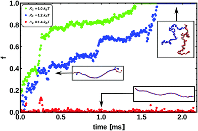Fig. 9 This figure shows the fraction of denatured base pairs f as a function of time and for different bond energies connecting the patches of paired bases, for a chain 300 bp long. Snapshots from simulations are also shown. The energies used range between K₂ = 1.0 k_BT and K₂ = 1.4 k_BT. We always observe that in linear dsDNA the denaturation process nucleates from the ends, as suggested by experiments.⁶⁹

Single stranded DNA (ssDNA) is much more flexible than its bound counterpart. In order to mimic this behaviour in our model, we eliminate both the dihedral and the Kratky–Porod interactions between nucleotides which are part of a “bubble” larger than two base-pairs. This results in single strands with a persistence length of around 2 bp which are extremely flexible, as one can appreciate from the snapshots in Fig. 9.

As previously mentioned, another way to denature DNA is by increasing the temperature of the system. We performed simulations where this pathway was adopted to denature our model DNA and found that the melting temperature is approximately 70 °C which is somewhat close but below the experimentally observed melting temperature.⁷⁰

We should point out here two limitations of the current model. First, while it can be used to study the reverse of partial denaturation by, for instance, non-monotonically tuning the value of K₂ or temperature, the current model cannot create hybridised molecules in which nucleotides partner up with nucleotides other than those to which they were bonded to start with. In other words, “secondary” structures and hairpins cannot be formed at this stage. Second, as previously mentioned, the model does not include sequence specificity, which is known to affect the local dynamics of denaturation. We aim to address both these aspects in the future. In regard to sequence specificity, this can be accounted for straightforwardly by defining two types of harmonic bonds connecting patches in the complementary strands and by using springs with different stiffness such that K₂(AT) < K₂(CG). Since stacking is also sequence-dependent we could, in a similar way, define different types of stacking (Morse) potentials with distinct parameters which can depend on the local sequence. In light of this, we expect that this model, thanks to its high scalability when run in parallel, will be of use to investigate the dynamics of denaturation of long dsDNA molecules, whether torsionally relaxed or supercoiled.

As a preliminary step to show that our model can readily take into account supercoiling, in Fig. 10 we present an example of simulated closed (ring) dsDNA. In particular, we consider a molecule 500 bp long and we initialise it with a linking number deficit of ΔLk = Lk₀ − Lk = −3 (47 turns instead of the usual 50 for a pitch of 10 bp). In a linear molecule this deficit would be quickly washed out by the free motion of the ends, whereas in a closed molecule the difference creates a negative supercoiling σ = ΔLk/Lk₀ ≃ −0.06 which is conserved throughout the dynamics. The supercoiling can then be distributed into the torsional or bending degrees of freedom as long as the White–Fuller theorem⁴⁷ is satisfied (see eqn (7)). Since the torsional stiffness of DNA is larger than the bending rigidity, much of the twist is quickly converted to writhe, as can be readily seen in Fig. 10.

Fig. 10 This figure shows the relaxation of a negatively supercoiled circular dsDNA. (left) The molecule (500 bp long) is initialised as a perfect ring from which three full turns are removed. (right) As the system evolves, the twist deficit is converted into writhe, and the molecule assumes stable buckled configurations. This behaviour is expected for a real dsDNA molecule because the torsional stiffness is larger than the bending rigidity.

6 Discussion

The interplay between the physics and biology of DNA is one of the most intriguing topics in biophysics. While computational models can strongly aid the understanding of this fascinating open problem, the computational resources for such an expensive task have traditionally been limited. Researchers often use either very detailed and accurate all-atoms models, which can only cover short time and length scales, or coarse-grained models, which can follow the evolution of the system for much longer times, but at the expense of neglecting key physical properties of dsDNA. Mesoscopic models have been recently proposed to fill in the gap between these two approaches: very successful and recent examples are the oxDNA code introduced in ref. 22, and the 3SPN.1 and 3SPN.2 codes.²⁴ However, such software has not yet been exported to a highly efficient and parallel environment. Here, we have proposed a mesoscopic coarse grained model that can be readily implemented at minimal cost into LAMMPS, one of the most popular molecular dynamics engines for atomistic and mesoscopic simulation.

6.1 Future improvements and limitations

Our model aims at bridging the gap between all-atoms and coarse-grained models for dsDNA; while it is currently less sophisticated than other mesoscopic models, such as oxDNA and 3SPN.2, most notably in the treatment of sequence specificity or hybridisation, this model exploits the scalability of LAMMPS, and is ideally suited to study problems such as DNA–protein interactions, or the denaturation of supercoiled DNA, where it is essential to consider long molecules, as well as to simultaneously model double-stranded and denatured regions.

This model can also be extended to include base-pair specificity, and variable salt or pH concentration, while allowing the user to reach biologically relevant time and length scales. In this paper we have shown that this model is capable of reproducing DNA melting and, more importantly, of tracking the dynamics of supercoiled molecules ∼1000 bp long for up to ∼2 ms. In the near future, we aim to use this model to investigate further the interplay between denaturation and supercoiling, especially in light of its connection to gene expression.^28,29

We should also highlight that the presented model has some notable limitations which arise from the compromise between accuracy and scalability. For instance, our model lacks the ability of reproducing realistic hybridisation events where distant parts of the chains can become bonded forming an intermediate hairpin. It also lacks sequence specificity, and a detailed description of counterion-mediated electrostatic interactions. While the choice of neglecting such events renders the modelling faster, it will be possible in principle to include them in the future, in cases where we are interested in hybridisation.

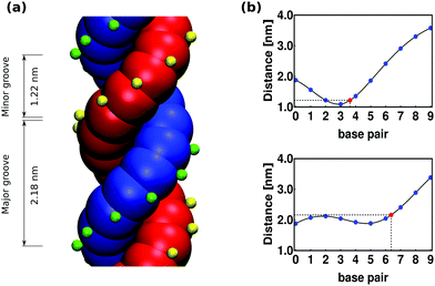
One of the improvements that can be readily made to the model is to account for the presence of major and minor grooves. Distinguishing between major and minor grooves may be important, for example, to capture the correct interaction of the chain with DNA-binding proteins, since these often bind selectively to one of the grooves. To address this issue, the model can be extended to include explicitly a phosphate group by means of a third monomer per nucleotide (see Appendix B for details). We note that without additional parametrization, the model is able to display the presence of asymmetric grooves with a total length of 1.22 nm (for the minor groove) and 2.18 nm (for the major groove).

Another important aspect worth considering in the future is the electrostatic interaction of DNA, either with itself or the environment. This is neglected in the current formulation of the model for the sake of efficient scalability of the parallelised code. Therefore the parameter tuning in Appendix A was carried out by implicitly assuming that the salt concentration corresponds to physiological conditions (0.15 M NaCl) and that the system is at room temperature (27 °C); under these conditions as previously mentioned the persistence length is l_p ≈ 50 nm. This, of course, will limit the range of applications of our model to systems where electrostatic properties are screened. Different approaches could be tested to address this aspect where needed. In ref. 71, for example, a Debye–Hückel potential is used to model DNA–DNA interactions, with an effective charge located at the backbone sites and an interaction radius depending on the salt concentration. This additional force field can be easily added to our model. A sligthly different approach could be to capture the effects of screened electrostatic repulsion by modulating the effective thickness of the chain in a similar way to that proposed in ref. 72 and 73. For the model we present here, it is possible to moderately modify the thickness of the chain by adjusting the excluded volume interaction between phosphates, when these are explicitly considered.

6.2 Computational scalability

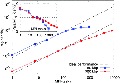
We extensively tested the scalability of the model (Fig. 11) by employing two benchmarks. They consisted both of linear, double-stranded DNA molecules of length of 600 bp each. The strands were initialised as a regular array of 10 × 10 or 40 × 40 strands, respectively to form a total system of 60 kbp and 960 kbp. The daily simulation times were derived from the loop timings of runs with 30 000 timesteps (60 kbp) and 10 000 timesteps (960 kbp) and were compared with those of a run with 24 processes (MPI-tasks), corresponding to one fully occupied node on ARCHER (see below). We made use of the “shift” load-balancing algorithm in LAMMPS, which re-positions the cutting planes between the single processes in order to mitigate a potential load imbalance between the individual processes (further details and full input files are available upon request). The model displays a very good speed-up up to hundreds of processes when deployed in parallel. These results are for so-called “strong scaling” where the number of processes is increased while the total problem size, in our case the number of nucleotides, is kept constant. The scaling tests were performed on ARCHER, a Cray XC30 supercomputer with 4920 compute nodes, each consisting of two 2.7 GHz 12-core Intel Ivy Bridge processors and Aries Interconnect (Dragonfly topology).

Fig. 11 This plot shows the scaling behaviour of the model and it is expressed as the simulation time achieved in a day of running time as a function of the number of parallel processes (MPI-tasks). Two different benchmarks were used to test the scalability: a small sample consisting of 60 kbp and a 16-times larger one with 960 kbp. The results are compared with the timings taken for a run with 24 processes for each benchmark, corresponding to one fully occupied node on the ARCHER XC30 architecture. This leads to parallel efficiencies (see inset) in excess of 100% for 1 and 8 processes. Total simulation times of up to 2 ms per day are feasible.

In particular, for the smaller problem size of 60 kbp we observe a parallel efficiency of about 50% at 512 MPI-tasks, allowing it to run for about 2 ms per day. More processes do not lead to a further speed-up and the parallel efficiency decreases rapidly due to the relatively small number of “atoms” per process (LAMMPS requires several hundred atoms per process to show good scaling behaviour). The larger benchmark of 960 kbp shows a parallel efficiency of about 50% at 2048 MPI-tasks, which permits simulation times of about 0.4 ms per day. Compared to the smaller benchmark the performance degrades more slowly in this case, making simulation times of up to 1 ms per day at 8192 MPI-tasks feasible. These results strongly encourage its use on a larger scale. Other existing models^22,23 might therefore be more suitable for studies of short DNA–DNA hybridisation leading to DNA origami and synthetic DNA assemblies. The model we presented here is instead more apt to study denaturation, supercoiling and DNA–protein interactions on larger length and time-scales as previously discussed.

Finally, exploiting the ability of LAMMPS to function as a library coupled to external programs, it is possible to design systems in which ATP-driven proteins interact with the model dsDNA. This paves the way to the attractive avenue of molecular dynamics simulation of large-scale out-of-equilibrium and biologically inspired systems, which are appealing to a broad range of researchers.

7 Conclusions

In summary, we have introduced a coarse-grained single-nucleotide model for dsDNA, which can be readily implemented in computationally efficient and parallelised engines, such as LAMMPS. We tuned the model in order to reproduce the crucial physical features of dsDNA such as bending and torsional rigidities. We then tested our model by simulating single-molecule experiments so as to independently check the parameterisation and the response of our model to external manipulation. Finally, we studied denaturation and the dynamics of supercoiled DNA. We have shown that this implementation can comfortably reach length and time scales that are relevant to both single molecule and biological experiments, therefore making our model interesting for applications. In the future we intend to refine this model and to extend it in order to study biologically-inspired out-of-equilibrium scenarios.

Appendix A: details of the model

The dynamics of the system are evolved using the Large-scale Atomic/Molecular Massively Parallel Simulator (LAMMPS) for which the scripts and input files employed in this work are available upon request. The position of the ith atom in the system, x_i, obeys the Langevin equationwhere γ is the friction coefficient and η_i is a stochastic noise term which satisfies 〈η_α(t)η_β(t′)〉 = 2γk_BTδ_αβδ(t − t′). The term ∇U_i is the gradient of the total potential U_i affecting bead i, whose contributions are described below.

A.1 Bonded interactions

The interactions between two consecutive beads in the same strand i and i + 1 are modelled by the Finite Extensible Non-linear Elastic (FENE) potential:where R₀ is the maximum bond length, K₁ is the spring constant and r is the Euclidean distance between bead i and bead i + 1. When summed to the Lennard-Jones potential (acting between any two beads), the minimum of this potential is located at r_min = 0.96 σ_s.

The “hydrogen bond” is mimicked by a truncated harmonic potential between the patches along the two strands (i and i′). This potential reads

if r ≤ r_c, and 0 otherwise. Here r represents the distance between patches i and i′, r₀ the equilibrium bond distance, K₂ the spring constant, and r_c is the critical distance above which the bond breaks. The minimum of this potential is located at r = r₀.

A.2 Non-bonded interactions

The excluded volume between beads is modelled via a truncated and shifted Lennard-Jones (LJ) potential. This potential acts between all possible pairs of beads so as to avoiding overlapping, and has the following form:for r < 2^1/6σ_s, and 0 otherwise. Here σ_s represents the diameter of a spherical bead, ε parametrises the strength of the repulsion and r is the Euclidean distance between the beads. The minimum of this potential is located at r = r_c = 2^1/6σ_s.

The dihedral interaction which regulates the handedness of the chain is given by:

U_dihedral(ϕ) = K₃[1 + cos(ϕ − d)], (13)

where ϕ is the angle between planes formed by the triplets described in Section 1 and d is a phase angle related to the equilibrium helical pitch.

The stacking of consecutive base-pairs is set by a combination of a Morse potential constraining the distance between consecutive patches

U_morse(r) = K₄[1 − e^{−λ(r−r₀)}]². (14)

where r₀ is the equilibrium distance. A stiff harmonic potential setting the angle α between the tangent along one strand and the vector joining a bead to its patch, imposes the planarity between consecutive patches.As described in Section 1 the minimum of this potential is set to α₀ = 90°.

Finally, the bending rigidity is given by a potential on the angle θ formed by three consecutive patches that reads

U_bending(θ) = K₆[1 + cos(θ)]. (16)

The parameters for each potential are reported in simulation units in Table 1.

Table 1 Parameter values in the model and expressed in simulation units

Interaction	Parameters
Backbone: Ubb	K 1 = 30, R0 = 0.6825, ε = 1 and σs = 0.4430
Hydrogen bond: Uhb	K 2 = 6, r0 = 0 and rc = 0.3
Steric: ULJ	ε = 1 and σs = 1
Dihedral: Udihedral	K 3 = 50, n = 1, and d = −144°
Morse: Umorse	K 4 = 30, λ = 8 and r0 = 0.34
Planarity: Uharmonic	K 5 = 200 and α0 = 90°
Bending: Ubending	K 6 = 52

---

A.3 Simulation units

Mapping the simulation units to physical ones can be done by setting the fundamental units: distance, energy and time. These are shown in Table 2. The chosen system of reference is a bath at room temperature T = 300 K and with the viscosity of water η = 1 cP. Finally, the numerical integration is performed in an NVT ensemble by a standard velocity-Verlet algorithm with integration time-step

Δt = 0.005τ_Br. (17)

Table 2 Mapping between simulation and physical units

Parameter	Experimental units
Distance (σs)	1 nm ≃ 3 bp
Energy (ε = kBT)	4.1419 × 10^−21 J
Force (F = ε/σs)	4.1419 × 10^−12 N
Mobility (μ = 1/(3πησs))	1.06 × 10^11 m Ns^−1
Diffusion (D = μkBT)	4.39 × 10^−10 m^2 s^−1
Time (τBr = σs^2/D)	2.28 × 10^−9 s

---

Appendix B: major and minor grooves

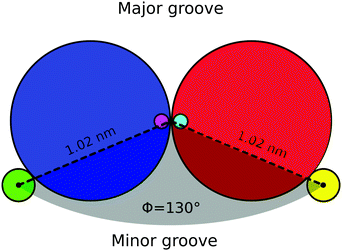
As mentioned in Section 6, the presence of grooves can be incorporated into our model by adding a third spherical monomer per nucleotide, representing the phosphate group. In Fig. 12 a top view of a base-pair is sketched. For one of the nucleotides, the excluded volume of the bead is shown in blue (with diameter of 1 nm), the patch is marked with pink (with no excluded volume) and its corresponding phosphate is shown in green at a distance of 1.02 nm from the center of the helix axis and with an excluded volume of 0.2 nm. Similarly, for the complementary nucleotide the excluded volume of the bead is shown in red, the patch in cyan and the phosphate in yellow. All the interactions mentioned in Section 2 remain unchanged.

Fig. 12 Sketch of a base-pair with the phosphate-group included explicitly. The bead-patch-phosphate complex (blue–pink–green for the first strand and red–cyan–yellow for the second strand) acts as a rigid body representing one nucleotide.

Including the phosphate in the model will add an additional degree of freedom per nucleotide, which is regulated by a harmonic angle interaction between two consecutive patches and a phosphate in the same strand, similar to the one imposing the planarity between consecutive nucleotides (see eqn (15)) and with the same value of the involved parameters (see Table 1). The smallest angle between the two phosphates in a base-pair and the helix axis (shown in light grey in Fig. 12) is ϕ = 130° and results in the minor groove when following the helical path of the dsDNA, as can be seen in Fig. 13(a). The conjugate angle is 230° and it gives rise to the major groove. If the pitch of the chain is 10 bp and therefore the helical angle between two consecutive base pairs is 36°, then the minor groove is made by 130/36 = 3.62 bp with a total length of around 3.62 × 0.34 = 1.2 nm. Correspondingly, the total length of the major groove is 2.2 nm.

Fig. 13 (a) Representation of the double-stranded DNA model with phosphates. Interactive and ghost beads are shown in red for one of the strands with the corresponding phosphates in yellow. The complementary strand and its phosphates are shown in blue and green respectively. The hydrogen bond sites (patches) are not depicted in this picture. (b) The top graphic shows (blue dots) the average distance between one phosphate chosen randomly from the red strand and the ten consecutive phosphates in the blue strand. The width of the minor groove can then be extracted from the interpolation curve (in black) at a distance of 3.62 bp, giving a value of 1.22 nm. This is when the green phosphate is on top of the previously chosen phosphate in the red strand, as depicted in (a). In a similar way the bottom graphic shows the average distance between one phosphate chosen randomly from the blue strand and the ten consecutive phosphates in the complementary strand. This time the major groove is extrapolated from the black curve at a distance of 6.38 bp, giving a width of 2.18 nm.

One way of determining the presence of grooves in our model is by comparing the average distance between one fixed phosphate chosen randomly from one of the strands and the ten consecutive phosphates in the complementary strand (including the one in the same base-pair). Since the grooves have a different size, the resulting plots differ from one another depending on the position of the fixed phosphate, whether it is on the first or the second, strand. In Fig. 13(b) we show these plots where the top graphic displays a global minimum that is related to the presence of the minor groove. In this plot, the blue dots represent the distance (averaged over time and base-pairs) between phosphates, measured from the simulation of a chain made by 300 bp. The spline interpolation of the blue dots is shown in black and the red point represents the inferred position of the minor groove, located at 3.62 bp with a distance of 1.22 nm. The bottom graphic in Fig. 13(b) is related to the major groove, in this case the interpolation gives a total width of 2.18 nm. The length of the grooves can be modified by changing the angle (ϕ) between the phosphates, but as the pitch remains constant the sum of the total widths of the grooves will always be 3.4 nm.

Appendix C: computing the torsional persistence length

To obtain the torsional properties of the DNA molecule described in Section 3.2 we consider a discrete elastic rod. As described in ref. 38, eqn (3) is an integral over the rate of rotation of the Darboux frame (or material frame) of reference with respect to the distance along the rod. We first find the discrete approximation to this in terms of the Euler angles α_n, β_n, γ_n which describe the rotation which generates the frame at segment n + 1 from that at segment n. To do this we make the approximation that the step size between segments is constant and denote it a; this gives
where twist angle between the frames is given by α_n + γ_n, so the total angle between m consecutive beads is given by . An appropriate measure of the thermal fluctuations about the equilibrium twist is given by the mean of the cosine of this angle; since this quantity will decrease with m, and we identify the decay constant as the torsional persistence length 〈cos Ω(m)〉 = e^−ma/l_τ. The ensemble average is found in the usual way by taking the integral over the phase space of the system; in the small a limit this gives

l_τ = 2C.

This is the case for an elastic rod; for the DNA molecule, the non-zero equilibrium twist between each base-pair will appear in the energy functional, so this must be subtracted from Ω(m) so that the ensemble average is a simple exponential decay. The Darboux frame at each DNA base-pair is given by the tangent vector, and the normal vector defined as the projection of the vector connecting the two beads onto the plane perpendicular to the tangent.

Appendix D: closure procedure for linear DNA

In this section we review the procedure to compute the linking number of an open segment of dsDNA. For clarity we report a schematic in Fig. 14. Given two curves C_R and C_B mapping the interval I = [0 : 1] → [Doublestruck R]³, it is possible to formally compute their linking number only if closed, i.e. C_R(0) = C_R(1) and C_B(0) = C_B(1). For a linear open segment of dsDNA, a pair of closed strands can be defined by considering the vectors tangent to the terminal pair of beads of the two single strands forming the dsDNA segment and extending the curves away from the pair of strands. After reaching a certain distance by following, for instance, t_1R and t_2R, one can close the contour by defining a vector f_R that joins the two new terminal beads (see Fig. 14). By following this procedure one can finally construct a pair of closed oriented curves γ_R and γ_B, for instance “stitching” C_R, t_1R, f_R, −t_2R, and similarly for the blue curve. Their linking number can be computed through the numerical evaluation of the double integralwhere r_R and r_B are the vectors defining the position of the segments along the curves γ_R and γ_B, respectively. If the centreline running through the pair of curves has no self-intersections (null writhe) then the linking number is equal to the twist. It is also worth mentioning that tightly wound curves, such as those obtained from dsDNA configurations, can lead to imprecise numerical evaluation of the integrals in eqn (18). In fact, the computation of Lk can become unreliable when |r_R − r_B| ≃ dr_R ≃ dr_B. The numerical evaluation can be arbitrarily improved by replacing the DNA backbones by contours more finely interspersed with points, i.e. enhancing the resolution of the integral by decreasing the infinitesimal element dr. Clearly, this can slow down the computation of Lk. We found a good compromise between precision and speed by adding three intermediate points every pair of beads for which we consistently measured the correct linking number during topology-preserving simulations (for instance by considering circular dsDNA).

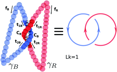Fig. 14 The “closure” procedure can be performed on a pair of linear open curves to construct a closed pair whose linking number can be formally defined through the Gauss' integral (see eqn (18)). In this case the curves are linked once. See text for further details.

Acknowledgements

This work was funded by ERC (Consolidator Grant 648050 THREEDCELLPHYSICS). OH acknowledges support from the EPSRC Reseach Software Engineer Fellowship Scheme (EP/N019180/1). This work used the ARCHER UK National Supercomputing Service. Y. A. G. F. acknowledges support from CONACyT PhD Grant 384582.

References

1. J. D. Watson and F. H. C. Crick, Nature, 1953, 171, 737–738.
2. M. Wilkins, A. Stokes and H. Wilson, Nature, 1953, 171, 738–740.
3. R. Franklin and R. Gosling, Nature, 1953, 172, 156–157.
4. C. R. Calladine, H. Drew, F. B. Luisi and A. A. Travers, Understanding DNA: the molecule and how it works, Elsevier Academic Press, 1997.
5. A. Bates and A. Maxwell, DNA topology, Oxford University Press, 2005.
6. G. Cavalli and T. Misteli, Nat. Struct. Mol. Biol., 2013, 20, 290–299.
7. C. A. Brackley, S. Taylor, A. Papantonis, P. R. Cook and D. Marenduzzo, Proc. Natl. Acad. Sci. U. S. A., 2013, 110, E3605–E3611.
8. P. R. Cook and D. Marenduzzo, J. Cell Biol., 2009, 186, 825–834.
9. P. R. Cook, Nat. Genet., 2002, 32, 347–352.
10. B. Alberts, A. Johnson, J. Lewis, D. Morgan and M. Raff, Molecular Biology of the Cell, Taylor & Francis, 2014, p. 1464.
11. M. E. Leunissen, R. Dreyfus, R. Sha, T. Wang, N. C. Seeman, D. J. Pine and P. M. Chaikin, Soft Matter, 2009, 5, 2422.
12. L. Di Michele and E. Eiser, Phys. Chem. Chem. Phys., 2013, 15, 3115–3129.
13. P. W. K. Rothemund, Nature, 2006, 440, 297–302.
14. C. K. McLaughlin, G. D. Hamblin and H. F. Sleiman, Chem. Soc. Rev., 2011, 40, 5647–5656.
15. T. E. Cheatham, 3rd, Curr. Opin. Struct. Biol., 2004, 14, 360–367.
16. E. Fadrná, N. Špačková, J. Sarzyñska, J. Koča, M. Orozco, T. E. Cheatham III, T. Kulinski and J. Šponer, J. Chem. Theory Comput., 2009, 5, 2514–2530.
17. M. Orozco, A. Noy and A. Pérez, Curr. Opin. Struct. Biol., 2008, 18, 185–193.
18. I. D'Annessa, A. Coletta, T. Sutthibutpong, J. Mitchell, G. Chillemi, S. Harris and A. Desideri, Nucleic Acids Res., 2014, 42, 9304–9312.
19. D. Michieletto, D. Marenduzzo and A. H. Wani, 2016, arXiv:1604.03041, 1–20.
20. A. Rosa and R. Everaers, PLoS Comput. Biol., 2008, 4, 1.
21. D. Michieletto, D. Marenduzzo and E. Orlandini, Proc. Natl. Acad. Sci. U. S. A., 2015, E5471–E5477.
22. T. E. Ouldridge, A. A. Louis and J. P. K. Doye, J. Chem. Phys., 2011, 72, 085101.
23. D. M. Hinckley, G. S. Freeman, J. K. Whitmer and J. J. de Pablo, J. Chem. Phys., 2013, 139, 144903.
24. J. J. de Pablo, Annu. Rev. Phys. Chem., 2011, 62, 555–574.
25. S. K. Nomidis, W. Vanderlinden, J. Lipfert and E. Carlon, 2016, arXiv:1603.00835, 1–12.
26. A. Prunell, Biophys. J., 1998, 74, 2531–2544.
27. J. J. Hayes, T. D. Tullius and A. P. Wolffe, Proc. Natl. Acad. Sci. U. S. A., 1990, 87, 7405–7409.
28. Y. Ding, C. Manzo, G. Fulcrand, F. Leng, D. Dunlap and L. Finzi, Proc. Natl. Acad. Sci. U. S. A., 2014, 111, 15402–15407.
29. C. A. Brackley, J. Johnson, A. Bentivoglio, S. Corless, N. Gilbert, G. Gonnella and D. Marenduzzo, Phys. Rev. Lett., 2016, 117, 018101.
30. S. Plimpton, J. Comput. Phys., 1995, 117, 1–19.
31. F. Ritort, J. Phys.: Condens. Matter, 2006, 18, R531–R583.
32. Z. Bryant, M. D. Stone, J. Gore, S. B. Smith, N. R. Cozzarelli and C. Bustamante, Nature, 2003, 424, 338–341.
33. S. Smith, Y. Cui and C. Bustamante, Science, 1996, 5, 795–799.
34. J. Lipfert, J. W. J. Kerssemakers, T. Jager and N. H. Dekker, Nat. Methods, 2010, 7, 977–980.
35. Z. Bryant, M. D. Stone, J. Gore, S. B. Smith, N. R. Cozzarelli and C. Bustamante, Nature, 2003, 424, 338–341.
36. T. R. Strick, J.-F. Allemand, D. Bensimon, R. Lavery and V. Croquette, Physica A, 1999, 263, 392–404.
37. J. Moroz and P. Nelson, Macromolecules, 1998, 9297, 6333–6347.
38. C. A. Brackley, A. N. Morozov and D. Marenduzzo, J. Chem. Phys., 2014, 140, 135103.
39. C. Bustamante, Z. Bryant and S. Smith, Nature, 2003, 421, 423–427.
40. C. Bustamante, J. Marko, E. Sigga and S. Smith, Science, 1994, 265, 1599–1600.
41. D. W. Michelle, Y. Hong, L. Robert, G. Jeff and M. B. Steven, Biophys. J., 1997, 72, 1335–1346.
42. S. Smith, L. Finzi and C. Bustamente, Science, 1992, 258, 1122–1126.
43. F. M. John and D. S. Erick, Macromolecules, 1995, 28, 8759–8770.
44. T. Odijk, Macromolecules, 1995, 28, 7016–7018.
45. C. Bustamante, S. Smith, J. Liphardt and D. Smith, Curr. Opin. Struct. Biol., 2000, 279–285.
46. C. Matek, T. Ouldridge, J. P. K. Doye and A. A. Louis, Sci. Rep., 2015, 5, 7655.
47. F. B. Fuller, Proc. Natl. Acad. Sci. U. S. A., 1978, 75, 3557–3561.
48. E. Orlandini, M. C. Tesi and S. G. Whittington, J. Phys. A: Math. Gen., 2000, 33, 181–186.
49. D. Michieletto, D. Marenduzzo, E. Orlandini, G. P. Alexander and M. S. Turner, ACS Macro Lett., 2014, 3, 255–259.
50. A. Vologodskii, Biophysics of DNA, Cambridge University Press, 2015.
51. C. Bouchiat, M. D. Wang, J. F. Allemand, T. Strick, S. M. Block and V. Croquette, Biophys. J., 1999, 76, 409–413.
52. L. Oroszi, P. Galajda, H. Kirei, S. Bottka and P. Ormos, Phys. Rev. Lett., 2006, 97, 1–4.
53. D. Poland and H. A. Scheraga, J. Chem. Phys., 1966, 45, 1464–1469.
54. J. T. O. Kirk, Biochem. J., 1967, 105, 673–677.
55. D. W. Gruenwedel and C.-h. Hsu, Biopolymers, 1969, 7, 557–570.
56. P. Botchan, J. C. Wang and H. Echols, Proc. Natl. Acad. Sci. U. S. A., 1973, 70, 3077–3081.
57. A. Kabakçiolu, E. Orlandini and D. Mukamel, Phys. Rev. E: Stat., Nonlinear, Soft Matter Phys., 2009, 80, 1–4.
58. G. Lia, D. Bensimon, V. Croquette, J.-F. Allemand, D. Dunlap, D. E. A. Lewis, S. Adhya and L. Finzi, Proc. Natl. Acad. Sci. U. S. A., 2003, 100, 11373–11377.
59. J.-H. Jeon, J. Adamcik, G. Dietler and R. Metzler, Phys. Rev. Lett., 2010, 105, 208101.
60. C. Lavelle, Curr. Opin. Genet. Dev., 2014, 25, 74–84.
61. J. J. Kozak and C. J. Benham, Proc. Natl. Acad. Sci. U. S. A., 1974, 71, 1977–1981.
62. C. J. Benham, Proc. Natl. Acad. Sci. U. S. A., 1979, 76, 3870–3874.
63. G. W. Hatfield and C. J. Benham, Annu. Rev. Genet., 2002, 36, 175–203.
64. E. Carlon, E. Orlandini and A. Stella, Phys. Rev. Lett., 2002, 88, 198101.
65. S. P. Mielke, N. Gronbech-Jensen, V. V. Krishnan, W. H. Fink and C. J. Benham, J. Chem. Phys., 2005, 123, 124911.
66. F. Sicard, N. Destainville and M. Manghi, J. Chem. Phys., 2015, 142, 034903.
67. H. Wang and C. J. Benham, PLoS Comput. Biol., 2008, 4, 0062–0076.
68. J. Wood, Biochem. J., 1974, 143, 775–777.
69. W. Beers, A. Cerami and E. Reich, Proc. Natl. Acad. Sci. U. S. A., 1967, 58, 1624–1631.
70. C. Schildkraut and S. Lifson, Biopolymers, 1965, 3, 195–208.
71. B. E. K. Snodin, F. Randisi, M. Mosayebi, P. Šulc, J. S. Schreck, F. Romano, T. E. Ouldridge, R. Tsukanov, E. Nir, A. A. Louis and J. P. K. Doye, J. Chem. Phys., 2015, 142, 234901.
72. V. Rybenkov, N. Cozzarelli and A. Vologodskii, Proc. Natl. Acad. Sci. U. S. A., 1993, 90, 5307–5311.
73. N. M. Toan and C. Micheletti, J. Phys.: Condens. Matter, 2006, 18, S269.

---