 Open Access Article
Creative Commons Attribution 3.0 Unported Licence
Mathematical model suitable for efficient simulation of thin semi-flexible polymers in complex environments
Jiří
Pešek
*a,
Pieter
Baerts
b,
Bart
Smeets
a,
Christian
Maes
b and
Herman
Ramon
a
aKU Leuven, BIOSYST-MeBioS, Kasteelpark Arenberg 30, B-3001 Leuven, Belgium. E-mail: jiri.pesek@biw.kuleuven.be
bKU Leuven, Instituut voor Theoretishe Fysica, Celestijnenlaan 200D, B-3001 Leuven, Belgium
First published on 1st March 2016
Abstract
We present an alternative approach to simulations of semi-flexible polymers. In contrast with the usual bead-rod compromise between bead-spring and rigid rod models, we use deformable cylindrical segments as basic units of the polymer. The length of each segment is not preserved with end points diffusing under constraints keeping the polymer chain nature intact. The model allows the simulation of tension transport and elasticity properties. In particular we describe a new cooperative regime in the relaxation of the polymer from its fully elongated configuration.
1 Introduction
Ever increasing interest in biological systems from the physical community has been pushing the boundaries of both theoretical and numerical methods. One specific area that is undergoing such a development is the physics of biopolymers with DNA as its most famous example. Other important examples of biopolymers include tubulin and F-actin. A common characteristic of the polymers mentioned above is that they belong to the class of thin long semi-flexible polymers, e.g. the width of F-actin is d = 6 nm, its typical length being L ≈ 1 μm and its persistence length![[small script l]](https://www.rsc.org/images/entities/char_e146.gif) p = 17.2 μm, for other examples see Andrews.1 Especially the small width-length ratio poses a remarkable challenge for simulations of systems consisting of such polymers. Moreover, these polymers naturally occur in dense highly connected active networks in the cytoskeleton, an environment that is rich in molecular motors, which exert forces exceeding the thermal forces due to collisions with particles in the solution. This leads to additional requirements on the stability of the used models. In this paper we present a model suitable for simulating polymers under these conditions.
p = 17.2 μm, for other examples see Andrews.1 Especially the small width-length ratio poses a remarkable challenge for simulations of systems consisting of such polymers. Moreover, these polymers naturally occur in dense highly connected active networks in the cytoskeleton, an environment that is rich in molecular motors, which exert forces exceeding the thermal forces due to collisions with particles in the solution. This leads to additional requirements on the stability of the used models. In this paper we present a model suitable for simulating polymers under these conditions.
The traditional approach to simulate polymers is based on bead-spring models like the Gaussian chain, the Zimm or Rouse model.1–4 The main advantage of such models is their relative simplicity and, at least in case of the Gaussian chain, many results can be obtained analytically.2,5 Despite many successful applications of such models, e.g. Jendrejack et al.6 and Mohammadinejad et al.,7 the main disadvantage is the large number of degrees of freedom necessary for the correct description of long thin polymers. In complex environments, the bead size and spacing between the beads has to be comparable with the diameter of the polymer, e.g. for L = 1 μm long actin filaments we need to have approximately 150 beads to represent a single polymer. This fact renders such models infeasible for the simulation of systems consisting of a large number of polymers. An interesting attempt to address this weakness of bead-spring models was presented by Panja et al.,8 who decompose the dynamics of a polymer into the dynamics of its normal modes. However the open question remains how to include large local forces, e.g. caused by molecular motors, in such a framework as they become non-local in the representation by normal modes. Another attempt at improving bead-spring models include modifications of the integration scheme.9
Another approach used to simulate large polymer networks is to consider the polymers as rigid rods.10 The main advantage of such an approach is to have faster simulations at the expense of neglecting deformations of single polymers. However as forces produced by molecular motors are of the order of ∥F∥ ∝ pN,11,12i.e. they exceed the usual thermal fluctuations, the assumption of rigidity of the polymers based solely on their persistence length may not suffice to correctly describe the behaviour of polymers in more violent environments, like in the cytoskeleton.
The class of bead-rod models is a natural compromise between bead-spring models and rigid rod models. It allows to preserve some details of the dynamics of single polymers, while it reduces the amount of necessary degrees of freedom. The simplest and most commonly used bead-rod model is a bead-spring model without hydrodynamical interactions and where collisions between polymers are treated based on a cylindrical rather than a spherical geometry. Random forces and friction applied to the beads also take into account the cylindrical geometry of the segments.12,13 Another issue with this approach is that it is necessary to properly renormalise the spring constant with the increasing length of segments.14 A different approach is taken in Somasi et al.4 or in Montesi et al.15 where instead of using bead-spring models, constraints are introduced to preserve the length of each segment.
In this paper we present an extensible cylinder chain model for polymers as an alternative to bead-rod models. The main difference with the bead-rod models is that we associate the degrees of freedom with extensible cylindrical segments rather than with beads, even though we represent the segments by the positions of their end points. The equations of motion for those points correspond to overdamped diffusion of a single cylinder,16,17 which can be seen by the presence of two independent thermal noise components per cylinder segment corresponding to both translational and rotational–extensional degrees of freedom. This is fundamentally different from bead-rod models.4,12,13,15 Lastly these segments are connected into chains by constraints posed on the positions of the end points of neighbouring segments. The length of a single segment is not preserved during the time evolution in our model, hence our model is more closely related to models used by Kim et al.13 or Gordon et al.12 with a finite tension propagation speed.
The paper is organized in the following manner: In Section 2 we derive from first principles the overdamped diffusion of a single stiff cylinder representing a single segment of the chain representing the whole polymer. In the next section, Section 3, we introduce constraints on the motion of single segments and the bending model thus concluding the presentation of the polymer model. Section 4 is the summary of our model in a form of a simulation scheme. Section 5 contains some of the basic tests of our model, including a comparison to the worm-like-chain (WLC). In Section 6 we apply our model to study the relaxation of polymers towards equilibrium and observe a new cooperative regime previously not discussed in the literature.
2 Overdamped diffusion of thin stiff cylinder
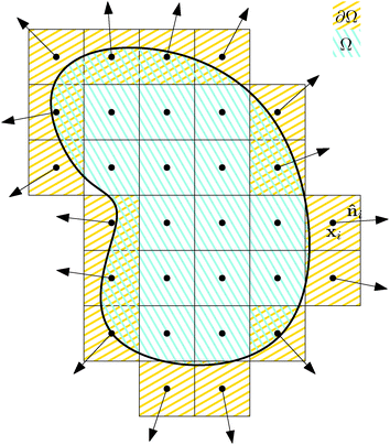
Our starting point is underdamped diffusion of rigid bodies submerged in an environment with constant temperature and viscosity. Even though there have been numerous studies on this subject, also in the context of rod-like polymers,2,16,17 here we present an alternative approach suited for performing simulations of very thin polymers, where the diameter of the polymer is almost negligible compared with the segments length, in an environment where large forces will be generated locally and/or high polymer densities are realised.We start with an overview of diffusion of rigid bodies, namely with the discretisation of a rigid body Ω into elements of constant volume Vi, see Fig. 1. Then we identify the relevant macroscopic degrees of freedom and extend the description to include deformations. In the end we take the continuous limit Vi → 0+ to obtain macroscopic equations describing the underdamped diffusion of stiff bodies followed by taking the overdamped limit.
Each discrete element i is characterized by its position xi, velocity vi, volume Vi, mass mi and, in case it belongs to the surface of the rigid body ∂Ω, by its normal vector to the surface ![[n with combining circumflex]](https://www.rsc.org/images/entities/b_i_char_006e_0302.gif) i.
i.
The time evolution of each internal element, i ∉ ∂Ω, is governed by the set of Lagrange's equations of the first kind
| dxi = vi dt, |
| mi dvi = Ftoti({xj},t) dt, |
We assume that the time evolution of surface elements, i ∈ ∂Ω, can be described by the Langevin equation
 | (1) |
![[n with combining circumflex]](https://www.rsc.org/images/entities/b_i_char_006e_0302.gif) i,t) corresponds to fluctuations caused by collisions with molecules of the surrounding liquid. Consequently, the noise applied to the element i always assumes the direction of the inner normal −
i,t) corresponds to fluctuations caused by collisions with molecules of the surrounding liquid. Consequently, the noise applied to the element i always assumes the direction of the inner normal −![[n with combining circumflex]](https://www.rsc.org/images/entities/b_i_char_006e_0302.gif) i. We further assume that the noise applied to different discrete elements is uncorrelated, hence
i. We further assume that the noise applied to different discrete elements is uncorrelated, henceWe remark here that in the whole paper, we are working within the framework of the Itô formalism.18
Note that the only difference between rigid and deformable bodies on this level of description is in the exchange of virtual forces representing the constraints by actual forces representing the elastic properties of deformable bodies.
![[n with combining circumflex]](https://www.rsc.org/images/entities/b_i_char_006e_0302.gif) i,t) → Wi′.
i,t) → Wi′.
2.1 Underdamped diffusion of a stiff cylinder
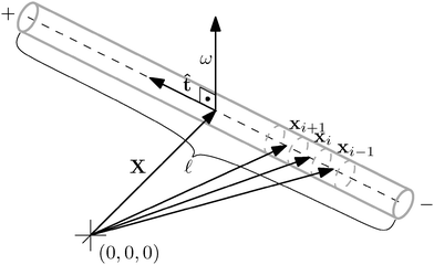
We apply the general framework introduced above to a thin, stiff cylinder. First, we consider the cylinder to be rigid and we will later release this constraint. The cylinder has an obvious set of symmetries: it is centrally symmetric as well as rotationally symmetric with respect to the axis![[t with combining circumflex]](https://www.rsc.org/images/entities/b_i_char_0074_0302.gif) . We assume the cylinder to be homogeneous, hence its centre of mass has to be at the same position as the symmetry centre X, i.e. it has to lie on the axis at one half of the cylinder's length
. We assume the cylinder to be homogeneous, hence its centre of mass has to be at the same position as the symmetry centre X, i.e. it has to lie on the axis at one half of the cylinder's length ![[small script l]](https://www.rsc.org/images/entities/char_e146.gif) . For these reasons, the natural macroscopic degrees of freedom consist of those describing the movement of the centre of mass and rotations around it.
. For these reasons, the natural macroscopic degrees of freedom consist of those describing the movement of the centre of mass and rotations around it.
By considering the cylinder to be thin we mean that any torque applied to the cylinder is negligible compared to the friction opposing it, so we can simplify our model just to include rotations around any axis perpendicular to the axis of the cylinder. In this assumption we deviate from the approach taken by Dhont17 and we will see later that it has a great effect on the relative simplicity of the eqn (14), describing the overdamped diffusion of a cylinder.
A consequence of this assumption is that we have to discretise the cylinder only along its axis, see Fig. 2. In that case the time evolution of all elements needs to be described by (1), although we have to replace the noise dWi′ with the one integrated along the element's surface dWi and subsequently the friction matrix γi′ by its effective counterpart γi. From symmetry then follows
where by xi ≈ ±
![[small script l]](https://www.rsc.org/images/entities/char_e146.gif)
![[t with combining circumflex]](https://www.rsc.org/images/entities/b_i_char_0074_0302.gif) /2 we denote the first and last discrete element representing the cylinder in the direction of
/2 we denote the first and last discrete element representing the cylinder in the direction of ![[t with combining circumflex]](https://www.rsc.org/images/entities/b_i_char_0074_0302.gif) .
.
Now we extend our description to include deformations. As we are trying to describe a single segment much shorter than the persistence length of the overall polymer ![[small script l]](https://www.rsc.org/images/entities/char_e146.gif) ≪
≪ ![[small script l]](https://www.rsc.org/images/entities/char_e146.gif) p we can neglect the bending of the cylinder and we do not need to apply the renormalisation procedure for the segment stiffness introduced by Gutjahr et al.14 as its effect will be negligible. The stiffness of the cylinder, characterized by its high Young's modulus E, is entering our equations twice. Firstly, the deformations in the direction perpendicular to the cylinder's axis are considered negligible as the width of the cylinder is small in comparison with the cylinders length. Secondly, the relaxation of the tension σ along the axis of the cylinder to a uniform profile occurs on a shorter time scale than the relaxation of velocities and positions, i.e. τrelax(σ) ≪ τrelax(vi) ≪ τrelax(xi). Hence we assume that the tension profile is homogeneous at every instant of time, so we need to add just a single degree of freedom in order to describe the longitudinal deformations, namely the relative stretching velocity λ defined as the longitudinal component of the relative end points velocity per unit length,
p we can neglect the bending of the cylinder and we do not need to apply the renormalisation procedure for the segment stiffness introduced by Gutjahr et al.14 as its effect will be negligible. The stiffness of the cylinder, characterized by its high Young's modulus E, is entering our equations twice. Firstly, the deformations in the direction perpendicular to the cylinder's axis are considered negligible as the width of the cylinder is small in comparison with the cylinders length. Secondly, the relaxation of the tension σ along the axis of the cylinder to a uniform profile occurs on a shorter time scale than the relaxation of velocities and positions, i.e. τrelax(σ) ≪ τrelax(vi) ≪ τrelax(xi). Hence we assume that the tension profile is homogeneous at every instant of time, so we need to add just a single degree of freedom in order to describe the longitudinal deformations, namely the relative stretching velocity λ defined as the longitudinal component of the relative end points velocity per unit length,
The velocity of each element vi can then be expressed as
| vi = V + ω × (xi − X) + (xi − X)λ, | (2) |
![[t with combining circumflex]](https://www.rsc.org/images/entities/b_i_char_0074_0302.gif) = 0. Such decomposition of the velocity automatically obeys all the necessary constraints on the thin stiff cylinder, hence we do not need to add any virtual forces to our description any more.
= 0. Such decomposition of the velocity automatically obeys all the necessary constraints on the thin stiff cylinder, hence we do not need to add any virtual forces to our description any more.
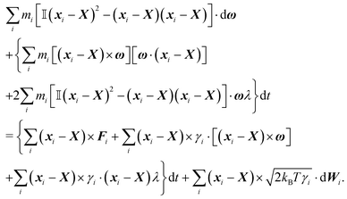
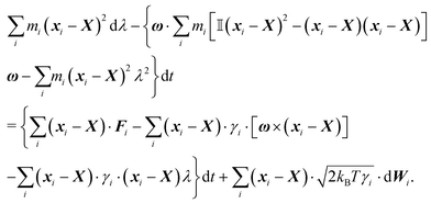
In order to obtain a set of equations for the macroscopic degrees of freedom we insert (2) into (1) and sum the set of equations with weights ∑dvi, ∑(xi − X) × dvi, ∑(xi − X)·dvi. These weights naturally decompose the motion of the cylinder into the translational, rotational and deformational degrees of freedom respectively. Let us define the total force F which is responsible for translations of a segment and the total effective “torque” T responsible for a segment's rotations and deformations as
![[t with combining circumflex]](https://www.rsc.org/images/entities/b_i_char_0074_0302.gif) . We need to stress here that the effective “torque” T is not a torque in its standard physical meaning. Its components are parallel with the applied force and, as will be demonstrated later in eqn (4), it fully characterizes both the moment of force and stress in the longitudinal direction. We also define effective friction matrices
. We need to stress here that the effective “torque” T is not a torque in its standard physical meaning. Its components are parallel with the applied force and, as will be demonstrated later in eqn (4), it fully characterizes both the moment of force and stress in the longitudinal direction. We also define effective friction matrices | (3) |
 | (4a) |
 | (4b) |
 | (4c) |
To have a closed set of equations we also need the following equations
dX = Vdt, d![[small script l]](https://www.rsc.org/images/entities/char_e146.gif) = = ![[small script l]](https://www.rsc.org/images/entities/char_e146.gif) λdt, d λdt, d![[t with combining circumflex]](https://www.rsc.org/images/entities/b_i_char_0074_0302.gif) = ω × = ω × ![[t with combining circumflex]](https://www.rsc.org/images/entities/b_i_char_0074_0302.gif) dt, dt, | (5) |
At this point we can substitute the friction coefficients obtained from the discretisation with the ones based on the actual Stokes drag on the cylinder19
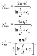 | (6) |
The remaining friction coefficient γ∥def will later, in the overdamped regime, be connected with the relaxation time of longitudinal perturbations τ![[small script l]](https://www.rsc.org/images/entities/char_e146.gif) .
.
2.2 Stiffness model
It is easy to determine the resulting total force F and effective “torque” T from external forces acting on particular points along the cylinder. The situation is a bit more complicated for internal elastic forces between the cylinder's elements. Here we demonstrate a general method of how to incorporate internal forces to the model in the very simple case of quadratic potentials between two neighbouring discrete elementswhere N is the number of discrete elements, k is the stiffness,
![[small script l]](https://www.rsc.org/images/entities/char_e146.gif) 0 is the equilibrium length of the cylinder and xN − x0 =
0 is the equilibrium length of the cylinder and xN − x0 = ![[small script l]](https://www.rsc.org/images/entities/char_e146.gif)
![[t with combining circumflex]](https://www.rsc.org/images/entities/b_i_char_0074_0302.gif) . The stiffness k is related to the Young's modulus E by
. The stiffness k is related to the Young's modulus E bywhere r is the cylinder radius. As we will show further on the scaling of the stiffness k by the total number of elements N is necessary for having a finite non-zero total elastic potential in the continuous limit N → ∞.
First let us write the contribution from the elastic forces Feli to a given element i
If we assume that cylinders are homogeneous at each time again, i.e. the corresponding relaxation time for non-homogeneous longitudinal deformations is much shorter than the typical time scale on which we observe our system, we obtain a much simpler formula for the potential
∇iVii−1 = −∇iVii+1 = k(![[small script l]](https://www.rsc.org/images/entities/char_e146.gif) − − ![[small script l]](https://www.rsc.org/images/entities/char_e146.gif) 0) 0)![[t with combining circumflex]](https://www.rsc.org/images/entities/b_i_char_0074_0302.gif) |
Hence elastic forces do not contribute to the total force applied on the cylinder, but they are included in the effective “torque”
This result is in good agreement with (4), as the elastic potential, without the help of other external force fields, cannot cause a displacement of the centre of mass nor a rotation of the object.
If we take the continuous limit of the total elastic potential
 | (7) |
Tel = −∂![[small script l]](https://www.rsc.org/images/entities/char_e146.gif) Vel( Vel(![[small script l]](https://www.rsc.org/images/entities/char_e146.gif) ) )![[small script l]](https://www.rsc.org/images/entities/char_e146.gif) ![[t with combining circumflex]](https://www.rsc.org/images/entities/b_i_char_0074_0302.gif) . . | (8) |
2.3 Representation by end points
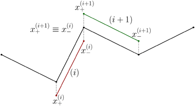
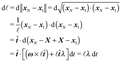
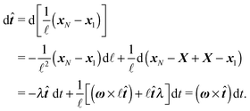
Although eqn (4) and (5) fully describe the underdamped diffusion of a single segment, it is more convenient for simulations to represent the motion of the whole segment by the motion of its end points, here denoted as “plus” x+ and “minus” x− end points, see Fig. 2. It follows from (5) that | (9) |
 | (10) |
where we can see that ω by definition obeys ω·
![[t with combining circumflex]](https://www.rsc.org/images/entities/b_i_char_0074_0302.gif) = 0.
= 0.
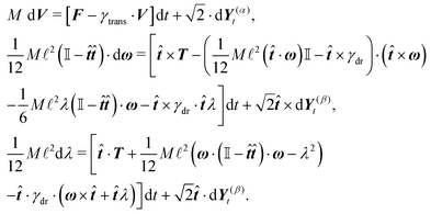
Using these expressions along with (5) we can combine all equations of motion of a segment (4) into those describing the motion of its end points
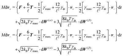 | (11) |
![[small script l]](https://www.rsc.org/images/entities/char_e146.gif) , γtrans(
, γtrans(![[t with combining circumflex]](https://www.rsc.org/images/entities/b_i_char_0074_0302.gif) ) and γdr(
) and γdr(![[t with combining circumflex]](https://www.rsc.org/images/entities/b_i_char_0074_0302.gif) ) are now function of the positions of the end points (10). We see that there is no longer a contribution from centrifugal and Coriolis forces as we are now describing the segments in an inertial frame of reference. Hence, the fact that the two points belong to the same segment is represented only by the friction terms and by autocorrelations between the velocities
) are now function of the positions of the end points (10). We see that there is no longer a contribution from centrifugal and Coriolis forces as we are now describing the segments in an inertial frame of reference. Hence, the fact that the two points belong to the same segment is represented only by the friction terms and by autocorrelations between the velocities ![[Doublestruck V]](https://www.rsc.org/images/entities/char_e179.gif) = (v+, v−),
= (v+, v−),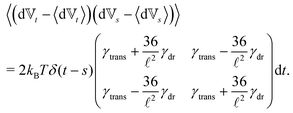 | (12) |
2.4 Overdamped limit
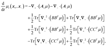
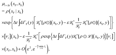
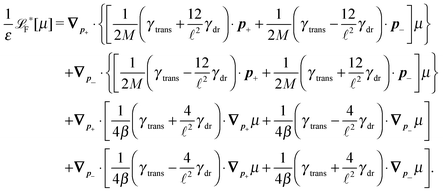
The simplest method to obtain an overdamped limit is by considering the acceleration terms MdvX to be negligible in (11). By this we obtain balance equations for all forces and moments which form a set of linear equations that can be solved with respect to the velocities.17 However such a simple method does not yield the correct result as our friction matrices depend on the orientation of the segment. Thus we need to proceed in a fashion similar to that of diffusion in a non-homogeneous environment,23 where the inhomogeneity is caused by the shape of the cylinder instead of external factors in the environment.A more refined method,24 suitable to more complex environments or configurations, starts from the assumption that canonical momenta have much shorter relaxation times than positions, τp ≪ τx. Then by observing the system on the time scale of positions, i.e. the slow degrees of freedom, we can expand the evolution equation in the degree of separation ε = τp/τx and obtain an autonomous Markovian dynamics for slow degrees of freedom up to linear order in ε, for technical details see Appendix C. Moreover in many cases the estimate for the relaxation time of canonical momenta can be obtained during the process, thus providing an explicit lower bound for the time step in simulations, see eqn (51).
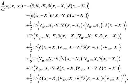
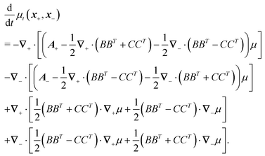
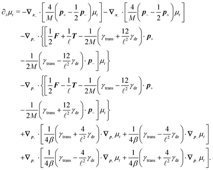
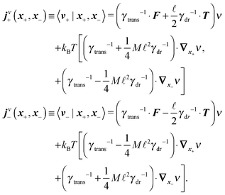
Following the second method and using that γtrans and γdr commute (3) and are invertible we obtain the Smoluchowski equation for the joint probability distribution μt(x+,x−)
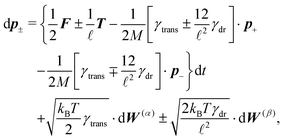
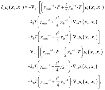 | (13) |
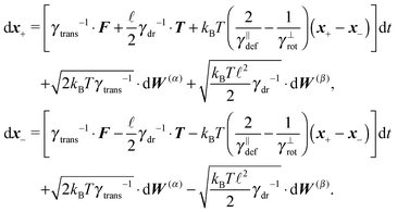 | (14) |
 | (15) |
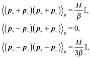
Similar to the velocities in the underdamped regime (12) we can see that positions ![[Doublestruck X]](https://www.rsc.org/images/entities/char_e17b.gif) = (x+,x−) in the overdamped limit are autocorrelated
= (x+,x−) in the overdamped limit are autocorrelated
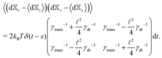 | (16) |
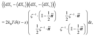 | (17) |
![[small script l]](https://www.rsc.org/images/entities/char_e146.gif) we briefly analyse the time evolution of the average length of the segments 〈
we briefly analyse the time evolution of the average length of the segments 〈![[small script l]](https://www.rsc.org/images/entities/char_e146.gif) 〉. It follows from the Smoluchowski eqn (13) that the time evolution of the mean value of length
〉. It follows from the Smoluchowski eqn (13) that the time evolution of the mean value of length ![[small script l]](https://www.rsc.org/images/entities/char_e146.gif) = ∥x+ − x−∥ is given by
= ∥x+ − x−∥ is given by | (18) |
which is negative. Hence without any potential opposing it, the segments always tend to increase their length indefinitely independently of the sign of the “thermal torque”, (15). Notice also that the mean value is taken with respect of the full probability distribution μ(x+,x−).
In the case where the only component of the effective “torque” parallel with the segment's axis is the contribution from the elastic potential (8), we can conclude that an equilibrium distribution of the length ρ(![[small script l]](https://www.rsc.org/images/entities/char_e146.gif) ) is given by
) is given by
 | (19) |
Quadratic stiffness potential. When there is a potential that is actually preserving a finite length of the segment
![[small script l]](https://www.rsc.org/images/entities/char_e146.gif) , the estimate for the relaxation time can be unrealistic as the first term on the right-hand side in eqn (18) cannot be neglected. To demonstrate this fact we provide a more realistic estimate for a quadratic potential, as was introduced in Section 2.2. First, we assume that we are in the low temperature regime where the system relaxes quickly to thermal equilibrium with equilibrium length
, the estimate for the relaxation time can be unrealistic as the first term on the right-hand side in eqn (18) cannot be neglected. To demonstrate this fact we provide a more realistic estimate for a quadratic potential, as was introduced in Section 2.2. First, we assume that we are in the low temperature regime where the system relaxes quickly to thermal equilibrium with equilibrium length ![[small script l]](https://www.rsc.org/images/entities/char_e146.gif) 0. Consequently, we can assume that any fluctuation that arises in the system is small and hence the probability distribution is close the equilibrium one. This enables us to decompose the full probability distribution μt into the equilibrium distribution (19) and a small correction Δμt, μt = ρ + Δμt. Also, we can assume that the correction Δμt is well localized around
0. Consequently, we can assume that any fluctuation that arises in the system is small and hence the probability distribution is close the equilibrium one. This enables us to decompose the full probability distribution μt into the equilibrium distribution (19) and a small correction Δμt, μt = ρ + Δμt. Also, we can assume that the correction Δμt is well localized around ![[small script l]](https://www.rsc.org/images/entities/char_e146.gif) 0. Hence, we can expand eqn (18) up to linear order in the length difference
0. Hence, we can expand eqn (18) up to linear order in the length differencefrom which a new estimate for the relaxation time immediately follows
 | (20) |
Remark: applications to nematic particles. Even though the focus of this article is mainly on the thin semi-flexible polymers, the model presented in this section is not restricted to this particular application and can be used to describe a behaviour of various physical and biological systems. The most prominent example might be elongated active swimmers like bacilli, which are a typical example of active nematic particles. Models for such systems where nematic particles have a constant speed, like the famous Vicsek model,31–33 can be mimicked by simply adding a non-potential force in the form F = F0
![[t with combining circumflex]](https://www.rsc.org/images/entities/b_i_char_0074_0302.gif) .
.
3 Diffusion of stiff chain
In the previous section we have described the dynamics of single segments, which we intend to use as basic building blocks for the description of semi-flexible polymers. Therefore the typical length of these segments has to be much shorter than the persistence length of the polymer. Consequently, we present one of the possible bending models to reflect the semi-flexibility of the polymer. Moreover in order to obtain a model for the full semi-flexible polymer we need to add suitable constraints on the independent movement of the segments. The presented approach of how to deal with such constraints is well known,4,15 however the actual form is heavily model dependent.3.1 Constraints
The basic constraint is that the positions of end points of neighbouring segments coincide at each instance of time, i.e. they have to move along the same trajectory,| x(i)− ≡ x(i+1)+, | (21) |
Virtual forces contribute to the total force and the total effective torque in the Langevin equations of motion (14) like any other force
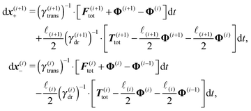 | (22) |
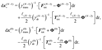 | (23) |
The constraint (21) is also valid for displacements, i.e. dx(i)− = dx(i+1)+, which provides us with the closure of eqn (22) and (23). Thus the virtual forces Φ(i) associated with constraints (21) are given as the solution of the set of linear equations
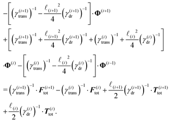 | (24) |
Notice that the virtual forces, obtained as a solution of this set of equations, are in fact random variables that depend on the actual realization of all coupled white noises. Moreover if we denote  we can clearly see that the structure on the left-hand side corresponds to the matrix multiplication of the vector of virtual forces Φ(i) with the tridiagonal symmetric block matrix
Moreover, the corresponding matrix is not necessarily positive definite. However, it is always invertible as any non-zero eigenvector corresponding to the zero eigenvalue would mean non-uniqueness in the resulting velocity profile and consequently in the non-uniqueness of positions. Such behaviour is deemed unphysical as one can expect that the problem is always well conditioned. From a computational point of view we can take advantage of algorithms like LDLT-decomposition, which scale linearly in time with the polymer length, to find the desired virtual forces.
3.2 Bending models
The usual model describing the bending of polymers is the worm-like chain (WLC) model34,35 with free energywhere a is the bending stiffness which can be later directly associated with the persistence length
![[small script l]](https://www.rsc.org/images/entities/char_e146.gif) p, r(s) is the curvature radius parametrized by the length s and L is the total length of the polymer. One of the few measurable quantities that is analytically accessible from the WLC is the mean squared end-to-end distance34
p, r(s) is the curvature radius parametrized by the length s and L is the total length of the polymer. One of the few measurable quantities that is analytically accessible from the WLC is the mean squared end-to-end distance34 | (25) |
Depending on the ratio between the total length L of the polymer and the persistence length we can distinguish two regimes by observing the squared end-to-end distance. One is the rod-like regime L≪![[small script l]](https://www.rsc.org/images/entities/char_e146.gif) p
p
| 〈R2〉 ≈ L2, |
![[small script l]](https://www.rsc.org/images/entities/char_e146.gif) p
p〈R2〉 ≈ 2L![[small script l]](https://www.rsc.org/images/entities/char_e146.gif) p, p, |
The simplest discretisation of the continuous WLC is the Kratky–Porod model36,37 with interaction potential
 | (26) |
![[t with combining circumflex]](https://www.rsc.org/images/entities/b_i_char_0074_0302.gif) i is the normalized tangential vector of i-th segment. However such a simple model has the disadvantage of enabling the segments to be aligned in an anti-parallel fashion. In the case of stiff semi-flexible polymers it is very unlikely that thermal fluctuations alone will ever cause such a perturbation, but in complex environments like the cytoskeleton we cannot exclude such possibility: external forces produced by molecular motors like Myosin-V can exceed thermal fluctuations by several orders of magnitude,11 and hence in the extreme case it can cause an anti-parallel alignment of some neighbouring segments. This situation corresponds to two segments occupying the same physical space, which is unphysical. Moreover, it also corresponds to the situation where the constraints (24) introduced in the previous subsections are not uniquely solvable, thus making the simulation unstable.
i is the normalized tangential vector of i-th segment. However such a simple model has the disadvantage of enabling the segments to be aligned in an anti-parallel fashion. In the case of stiff semi-flexible polymers it is very unlikely that thermal fluctuations alone will ever cause such a perturbation, but in complex environments like the cytoskeleton we cannot exclude such possibility: external forces produced by molecular motors like Myosin-V can exceed thermal fluctuations by several orders of magnitude,11 and hence in the extreme case it can cause an anti-parallel alignment of some neighbouring segments. This situation corresponds to two segments occupying the same physical space, which is unphysical. Moreover, it also corresponds to the situation where the constraints (24) introduced in the previous subsections are not uniquely solvable, thus making the simulation unstable.
One can argue that forces exerted by molecular motors are mainly tangential to the polymer. However, in dense complex networks, micro-filaments of molecular motors like Myosin-II, that have heads on both ends of their polymer chain,38 can be attached to two polymers at once. As two polymers generally are not parallel, the force exerted tangential to one polymer is translated to the other one as a force with a non-negligible perpendicular component.
Moreover, Myosin-II micro-filaments have a structure resembling a semi-flexible polymer.38 Hence they represent another example of a system subjected to large forces and as such is suitable to be described by the model presented here and which is subjected to large forces, although in the scope of this article we restricted ourselves to more common examples of polymers like F-actin and DNA.
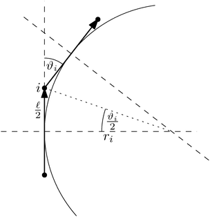
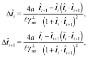
As our aim is to provide a model suitable for such violent environments we need to address this stability issue. An improved model is obtained by choosing a different discretisation scheme. Notably we assume a constant curvature between the centres of two neighbouring segments which is equal to the radius of the inscribed circle, while at the same time we assume the polymer length between the centre of two neighbouring segments to be constant and equal to ![[small script l]](https://www.rsc.org/images/entities/char_e146.gif) , see Fig. 4. This leads to the bending potential
, see Fig. 4. This leads to the bending potential
 | (27) |
This particular choice of discretisation resembles the behaviour of the Kratky–Porod model for small angles, as we have shown in Fig. 5, and for angles close to π it diverges, thus preventing the anti-alignment.
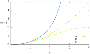 | ||
Fig. 5 Illustration of the dependency of the bending potential on the angle in different models. We fix  . Case A is the Kratky–Porod model as stated in (26), case B is the quadratic approximation of the Kratky–Porod model, . Case A is the Kratky–Porod model as stated in (26), case B is the quadratic approximation of the Kratky–Porod model,  and case C is the improved bending model given by (27). and case C is the improved bending model given by (27). | ||
It can be shown that the effective “torque” applied on a single segment and caused by a single joint (i,i + 1) is in general given by
where ∇
![[t with combining circumflex]](https://www.rsc.org/images/entities/b_i_char_0074_0302.gif) i is the gradient with respect to the normalized i-th segment's orientation vector
i is the gradient with respect to the normalized i-th segment's orientation vector ![[t with combining circumflex]](https://www.rsc.org/images/entities/b_i_char_0074_0302.gif) i. Notice that T(i)b·
i. Notice that T(i)b·![[t with combining circumflex]](https://www.rsc.org/images/entities/b_i_char_0074_0302.gif) i = 0. For the improved Kratky–Porod model (27) it yields
i = 0. For the improved Kratky–Porod model (27) it yields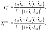 | (28) |
4 Simulation scheme
To summarize our model we present a step by step overview of the integration scheme of the model presented in this paper. Let us note that we employ the Euler–Maruyama integration scheme as a basic integration method.(1) For each segment the random effective “torque” and force are generated according to eqn (14):
where Δt is the used time step.
(2) For each segment the thermal effective “torque” T(i)thermal is evaluated according to the eqn (15).
(3) For each segment the elastic effective “torque” T(i)el is evaluated according to the eqn (8).
(4) For each joint the bending effective “torques” T(i)b, T(i+1)b are evaluated according to eqn (28).
(5) All other external forces applied to the segment, like the repulsion of polymers or forces exerted by molecular motors, not explicitly discussed in this paper, or the presence of optical tweezers, see Section 6, are evaluated and included
where r(i)α is the projection of the point where the force is applied xα onto the segments axis
(6) Virtual forces per joint Φ(i), see eqn (24), are evaluated based on the total forces and total effective “torques” per segment
| F(i)tot = F(i)rand + F(i)thermal + F(i)el + F(i)ext, |
| T(i)tot = T(i)rand + T(i)thermal + T(i)el + T(i)b + T(i)ext. |
(7) Positions are updated according to eqn (22) and (23) by using the forward Euler(–Maruyama) scheme.
In order to be in the overdamped regime we need to make sure that the time step is bigger then the lower bound given by the relaxation time of canonical momenta, see eqn (51).
4.1 Time complexity
The most complex task in the basic simulation scheme is the determination of the virtual forces that are binding the polymer together (step 6). It was discussed in Section 3.1 that this task has a linear time complexity in the number of segments per polymer, hence the full simulation scheme overall scales linearly with the total number of segments presented in the simulation. Therefore, it belongs to the same complexity class of algorithms as the traditional bead-spring approach of the model presented by Montesi et al.15 The main difference usually is the pre-factor which, when compared to the most simple bead-spring model, will be much larger in our case, because for each segment we need to generate two random numbers, as opposed to one in case of the bead-spring model (step 1), we need to perform the LDLT decomposition of the (3 × 3) matrices along with multiple matrix multiplications (step 6), etc. However the possibility to scale the length of the segments and thus decreasing the number of segments in the model can compensate the higher cost per single segment. The key parameter of the system which determines the maximal possible advantage of our model with respect to the traditional bead-spring model is the ratio of the persistence length to the diameter of the polymer
 ![[small script l]](https://www.rsc.org/images/entities/char_e146.gif) p/d. This is caused by the fact that in the traditional bead-spring approach the beads need to be spaced much less than 2d apart in order to avoid the possibility of two polymers passing through each other, while the size of the segment is limited by the persistence length
p/d. This is caused by the fact that in the traditional bead-spring approach the beads need to be spaced much less than 2d apart in order to avoid the possibility of two polymers passing through each other, while the size of the segment is limited by the persistence length ![[small script l]](https://www.rsc.org/images/entities/char_e146.gif) p.
p.
The second factor contributing to the efficiency of a given algorithm is how large the time step can be for a given set-up. The maximal allowed time step is determined by multiple factors, which can be split into two categories: the desired resolution of the simulation (both spatial and time) and the stability of the simulation. While the first category is determined solely by the considered set-up, the latter is determined only by physical properties and interactions in the system. Surprisingly, this means that the maximal time step also depends on the chosen segment length.
Some of these constraints are summarized for both the model presented here and the bead-spring model in Table 1, where the row labelled translations is the estimate of the maximal time step based on the requirement to prevent translational thermal forces to cause two segments to pass through each other in single time step without colliding. From the stochastic nature of these forces, the additional parameter cσ determining the confidence interval of the estimate, is needed. For further details we refer to Appendix D. The row labelled rotations is similar to that of translations but now with respect to thermal rotational forces. Diffusion is the estimate of the maximal time step for all thermal forces combined. This estimate is based on autocorrelations (16). γ* is the effective friction matrix, see (56) for exact expressions. Stiffness in the third row corresponds to the upper bound on the time step. This stems from the requirement that the reaction of the elastic potential (7) to the perturbation cannot cause an even bigger perturbation. For bending in row four, a similar requirement applies but now for the action of the bending potential (27). From the asymptotic behaviour of the estimates on the upper bound of the time step we see that the maximal time step achievable, for an arbitrarily large segment length ![[small script l]](https://www.rsc.org/images/entities/char_e146.gif) 0, is determined by the relaxation time of the longitudinal deformation τ
0, is determined by the relaxation time of the longitudinal deformation τ![[small script l]](https://www.rsc.org/images/entities/char_e146.gif) . However in the typical case of stiff thin polymers these estimates are (much) higher than those limiting the bead-spring model mainly due to the increased friction, thus boosting the efficiency of the approach discussed here.
. However in the typical case of stiff thin polymers these estimates are (much) higher than those limiting the bead-spring model mainly due to the increased friction, thus boosting the efficiency of the approach discussed here.
![[small script l]](https://www.rsc.org/images/entities/char_e146.gif) 0 ≫ d
0 ≫ d
In case pairwise interactions (e.g. Coulomb or Debye–Hückel electrostatic interaction) are present, the time to evaluate them depends quadratically on the number of elements, thus shifting the time complexity of the whole simulation up to a quadratic scaling in the worst case scenario. Hence purely by increasing the segment length, thus decreasing the number of elements in the simulation, can lead to a significant improvement, albeit sometimes at the cost of a more complex interaction potential.
5 Model performance
We demonstrate our simulation method by applying it on F-actin, which is a typical thin, d = 6 nm, stiff,![[small script l]](https://www.rsc.org/images/entities/char_e146.gif) p = 17.6 μm, polymer. The common parameters of all simulations are listed in Table 2. The value relaxation time of longitudinal deformations for single segment τ
p = 17.6 μm, polymer. The common parameters of all simulations are listed in Table 2. The value relaxation time of longitudinal deformations for single segment τ![[small script l]](https://www.rsc.org/images/entities/char_e146.gif) was chosen arbitrarily as there, to the best knowledge of authors, are no experimental data available. The aim was to have the highest value possible in order to achieve large time steps while preserving the stability of simulation. After couple of trials, the value listed in Table 2 was chosen. Relaxation times for the canonical momenta (51) can be evaluated from these parameters
was chosen arbitrarily as there, to the best knowledge of authors, are no experimental data available. The aim was to have the highest value possible in order to achieve large time steps while preserving the stability of simulation. After couple of trials, the value listed in Table 2 was chosen. Relaxation times for the canonical momenta (51) can be evaluated from these parameters| τFtrans,⊥ = 2.15 ps, τFtrans,∥ = 1.35 ps, |
| τFrot = 0.33 ps, τFdef = 0.04 ps. |
| d | 6 nm | Thickness of F-actin polymer40 |
![[small script l]](https://www.rsc.org/images/entities/char_e146.gif) p p |
17.2 μm | Persistence length of actin1,41,42 |
| k | 48.7 pN nm−1 | Stretching stiffness40,43 |
| c | −0.114 | Correction coefficient for γ∥trans, see (6),19–21 |
| c ⊥ | 0.886 | Correction coefficient for γ⊥trans, see (6),19–21 |
| c r | −0.447 | Correction coefficient for γ⊥rot, see (6),19–21 |
![[small script l]](https://www.rsc.org/images/entities/char_e146.gif) 0 0 |
360 nm | Single segment equilibrium length |
| Δt | 10−2 μs | Simulation time step |
τ
![[small script l]](https://www.rsc.org/images/entities/char_e146.gif)
|
0.1 μs | Relaxation time of a single segment longitudinal deformations, see eqn (20) and main text |
| k B T | 4.28 pN nm | Temperature of the environment (T = 310 K) |
| η | 1.71 × 10⁻³ pN μs nm−2 | Viscosity of the environment19 |
We can see that we are truly in the overdamped regime as the time step Δt is much bigger than any of the relaxation times. The mass of a single segment was assumed to be M = 1.26 MDa. All simulations presented here were created using the Mpacts framework.39
5.1 Speed comparison
In the first set of tests we provide a practical comparison between the time complexity of the model proposed here and the bead-spring model with spacing of the beads![[small script l]](https://www.rsc.org/images/entities/char_e146.gif) 0 = d. First we simulate the polymer with the contour length of 1.2 μm using the bead-spring model with 201 beads and using time step Δt = 10 ps for a total simulation time of T = 10 ms thus creating the baseline for comparison. Subsequently, we simulate the same polymer using the model introduced here with different segment lengths
0 = d. First we simulate the polymer with the contour length of 1.2 μm using the bead-spring model with 201 beads and using time step Δt = 10 ps for a total simulation time of T = 10 ms thus creating the baseline for comparison. Subsequently, we simulate the same polymer using the model introduced here with different segment lengths ![[small script l]](https://www.rsc.org/images/entities/char_e146.gif) 0 while maintaining the contour length and taking the same time step Δt = 10 ps and the same total simulation time T = 10 ms. The result of this comparison is shown in Fig. 6, where the speed-up is given as the ratio of the simulation duration† of our model and the bead-spring model. We can see that the maximal speed achieved was more than 10× higher than for the bead-spring model, when the full polymer was represented by a single segment. From the same figure we can also obtain the information about the overhead of the algorithm presented in Section 4. We see that the simulation containing 120 segments is approximately as fast as the simulation of the bead-spring model with 201 beads thus being about 40% slower per element than the bead-spring model. Moreover the slower increase of the speed for longer segments, which deviates from the linear scaling, can be attributed to the overhead of the simulation toolbox for a low number of elements. Unfortunately this bias is unavoidable in this comparison, because increasing the number of elements for long segments to sufficient numbers, e.g. by increasing the number of non-interacting polymers, will lead to impractical times necessary for the simulation of the bead-spring model of the actin polymer.
0 while maintaining the contour length and taking the same time step Δt = 10 ps and the same total simulation time T = 10 ms. The result of this comparison is shown in Fig. 6, where the speed-up is given as the ratio of the simulation duration† of our model and the bead-spring model. We can see that the maximal speed achieved was more than 10× higher than for the bead-spring model, when the full polymer was represented by a single segment. From the same figure we can also obtain the information about the overhead of the algorithm presented in Section 4. We see that the simulation containing 120 segments is approximately as fast as the simulation of the bead-spring model with 201 beads thus being about 40% slower per element than the bead-spring model. Moreover the slower increase of the speed for longer segments, which deviates from the linear scaling, can be attributed to the overhead of the simulation toolbox for a low number of elements. Unfortunately this bias is unavoidable in this comparison, because increasing the number of elements for long segments to sufficient numbers, e.g. by increasing the number of non-interacting polymers, will lead to impractical times necessary for the simulation of the bead-spring model of the actin polymer.
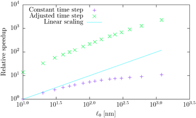 | ||
| Fig. 6 The log–log plot of the measured relative speed-up of the presented model for various segment lengths with respect to the bead-spring model based on the simulation of a single polymer with a contour length of L = 1.2 μm. The first data set uses the same time step Δt = 10 ps for all simulations, while the second data set increases the time step for each simulation according to the speed-up row of Table 3, thus preserving the minimal upper bound of the time step to the actual time step ratio. | ||
As we have discussed in Section 4.1, the maximal possible time step also depends on the segment length. In order to illustrate this issue we have listed estimates for maximal time steps, see Table 1, for various segment lengths in Table 3,‡ where we used the confidence interval 3σ, i.e. cσ = 3. There we can see that for short segment lengths the main limiting factor is the high bending rigidity. As the segment length increases the limitation caused by the bending rigidity quickly fades away due to its scaling as ![[small script l]](https://www.rsc.org/images/entities/char_e146.gif) 04/ln(
04/ln(![[small script l]](https://www.rsc.org/images/entities/char_e146.gif) 0/d), see Table 1. Hence, in the intermediate range of segment lengths, diffusion becomes the main limiting factor for the maximal time step. Namely, thermal fluctuations of the segments' length combined with translational Brownian motion along the segments' axis become the main limiting factors in this range. For long segments, we reach the saturation point, where we cannot increase the time step over a certain threshold. In case of F-actin the threshold is given by the relaxation time for longitudinal deformations, Δt ≪ 2τ
0/d), see Table 1. Hence, in the intermediate range of segment lengths, diffusion becomes the main limiting factor for the maximal time step. Namely, thermal fluctuations of the segments' length combined with translational Brownian motion along the segments' axis become the main limiting factors in this range. For long segments, we reach the saturation point, where we cannot increase the time step over a certain threshold. In case of F-actin the threshold is given by the relaxation time for longitudinal deformations, Δt ≪ 2τ![[small script l]](https://www.rsc.org/images/entities/char_e146.gif) . Hence the maximal speed-up theoretically achievable for the model presented in this paper by increasing the time step is more than 350×, i.e. more than two orders of magnitude. This can significantly enhance the performance of the overall simulation as is demonstrated in Fig. 6, where after adjusting the time step according to Table 3, we have achieved the maximal simulation speed-up of more than 2000× compared to the bead-spring model.
. Hence the maximal speed-up theoretically achievable for the model presented in this paper by increasing the time step is more than 350×, i.e. more than two orders of magnitude. This can significantly enhance the performance of the overall simulation as is demonstrated in Fig. 6, where after adjusting the time step according to Table 3, we have achieved the maximal simulation speed-up of more than 2000× compared to the bead-spring model.
| Bead-spring model | Segment length [nm] | ||||||||||
|---|---|---|---|---|---|---|---|---|---|---|---|
| 10 | 20 | 30 | 40 | 80 | 150 | 300 | 600 | 1200 | 2400 | ||
| Translations | 0.01130 | 0.0316 | 0.023 | 0.025 | 0.028 | 0.041 | 0.061 | 0.099 | 0.168 | 0.29 | 0.51 |
| Rotations | — | 0.1311 | 0.022 | 0.022 | 0.023 | 0.031 | 0.045 | 0.072 | 0.121 | 0.21 | 0.36 |
| Diffusion | — | 0.0158 | 0.012 | 0.013 | 0.014 | 0.020 | 0.030 | 0.050 | 0.084 | 0.15 | 0.26 |
| Stiffness | 0.00199 | 0.1993 | 0.200 | 0.200 | 0.200 | 0.200 | 0.200 | 0.200 | 0.200 | 0.20 | 0.20 |
| Bending | 0.00057 | 0.0076 | 0.010 | 0.034 | 0.086 | 0.932 | 8.903 | 113.952 | 1.5 × 10³ | 20.8 × 10³ | 0.29 × 10⁶ |
| Speed-up | — | 13.4 | 18.1 | 22.1 | 24.8 | 35.7 | 53.3 | 87.2 | 147.5 | 255.5 | 351.8 |
5.2 Diffusive properties of segments
Here we evaluate the rotational diffusion of free independent segments where translations of the segments are disabled, hence the equations of motion (14) simplify toIt can be shown that the mean orientation of the segments relaxes towards equilibrium, i.e. to a uniform distribution of orientations, 〈![[t with combining circumflex]](https://www.rsc.org/images/entities/b_i_char_0074_0302.gif) 〉 = 0, independent of the specific choice of the elastic potential (8) as
〉 = 0, independent of the specific choice of the elastic potential (8) as
 | (29) |
![[t with combining circumflex]](https://www.rsc.org/images/entities/b_i_char_0074_0302.gif) 〉t=0 = êx, see Fig. 7. The count of segments N is sufficiently high in order to have a reasonably large statistical ensemble for evaluation. The rotational relaxation time is found to be τr = 2.685 ± 0.028 ms which is in good agreement with the theoretical prediction τ = 2.676 ms. Moreover variances of the mean orientations' components converge to
〉t=0 = êx, see Fig. 7. The count of segments N is sufficiently high in order to have a reasonably large statistical ensemble for evaluation. The rotational relaxation time is found to be τr = 2.685 ± 0.028 ms which is in good agreement with the theoretical prediction τ = 2.676 ms. Moreover variances of the mean orientations' components converge to  , whose value is obtained from the uniform distribution of orientations.
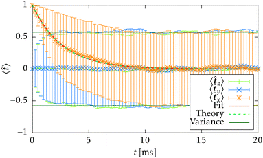 | ||
Fig. 7 Simulation of rotational diffusion for N = 728 independent segments, starting from the initial orientation ![[t with combining circumflex]](https://www.rsc.org/images/entities/b_i_char_0074_0302.gif) (t = 0) = êx. The translational diffusion is disabled in the simulation program for this purpose. The estimated rotational relaxation time τestr = 2.685 ± 0.028 ms is in good agreement with the theoretical prediction (29)τr = 2.676 ms. (t = 0) = êx. The translational diffusion is disabled in the simulation program for this purpose. The estimated rotational relaxation time τestr = 2.685 ± 0.028 ms is in good agreement with the theoretical prediction (29)τr = 2.676 ms. | ||
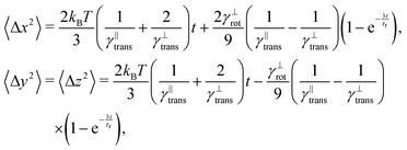
The second test verifies the translational properties of the segments that are also undergoing rotational diffusion. Starting from the same initial configuration, i.e. 〈![[t with combining circumflex]](https://www.rsc.org/images/entities/b_i_char_0074_0302.gif) 〉t=0 = êx, we let the particles evolve according to the complete equations of motion (14) with zero external force and torque. We shall observe the transition from inhomogeneous diffusion
〉t=0 = êx, we let the particles evolve according to the complete equations of motion (14) with zero external force and torque. We shall observe the transition from inhomogeneous diffusion
 | (30) |
 | (31) |
 | (32) |
![[t with combining circumflex]](https://www.rsc.org/images/entities/b_i_char_0074_0302.gif) 〉 = êx. In Fig. 8 we can see that the full time range solution agrees well with the simulation.
〉 = êx. In Fig. 8 we can see that the full time range solution agrees well with the simulation.
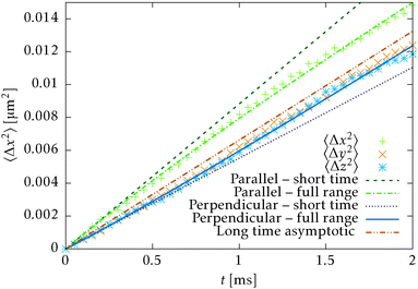 | ||
Fig. 8 Comparison of the simulation of the mean square displacement of N = 728 independent segments with short time (30), long time (31) and full range (32) theoretical predictions. The mean square displacement is evaluated in all principal directions, i.e. parallel and perpendicular to the initial orientation ![[t with combining circumflex]](https://www.rsc.org/images/entities/b_i_char_0074_0302.gif) (t = 0) = êx. Note that the long range and full range predictions will be asymptotically parallel for large times. (t = 0) = êx. Note that the long range and full range predictions will be asymptotically parallel for large times. | ||
5.3 Equilibrium squared end-to-end distance of a single polymer
In a first simulation of the full polymer, we investigate the convergence to equilibrium of a free single polymer. The initial configuration is that of a straight polymer, ∀i, j:![[t with combining circumflex]](https://www.rsc.org/images/entities/b_i_char_0074_0302.gif) i =
i = ![[t with combining circumflex]](https://www.rsc.org/images/entities/b_i_char_0074_0302.gif) j, with segment lengths
j, with segment lengths ![[small script l]](https://www.rsc.org/images/entities/char_e146.gif) equal to the equilibrium segment length
equal to the equilibrium segment length ![[small script l]](https://www.rsc.org/images/entities/char_e146.gif) 0. In other words, the polymer's initial configuration corresponds to the configuration with the lowest possible energy or the configuration at T = 0 K. The polymer is then let to thermalise with the environment for 1 s. Let us note that for this test we artificially decreased the viscosity of the environment to η = 1.71 × 10⁻⁴ pN μs nm−2, i.e. ten times lower than the value listed in Table 2, in order to decrease the relaxation time. The mean squared end-to-end distance 〈R2〉 is estimated based on the ergodic average over the time interval of 1 s
0. In other words, the polymer's initial configuration corresponds to the configuration with the lowest possible energy or the configuration at T = 0 K. The polymer is then let to thermalise with the environment for 1 s. Let us note that for this test we artificially decreased the viscosity of the environment to η = 1.71 × 10⁻⁴ pN μs nm−2, i.e. ten times lower than the value listed in Table 2, in order to decrease the relaxation time. The mean squared end-to-end distance 〈R2〉 is estimated based on the ergodic average over the time interval of 1 s | (33) |
Our simulation results are compared with theoretical prediction for the WLC (25), see Fig. 9. We can see that the results comply very well with the theoretical prediction for polymers shorter than the persistence length, L < ![[small script l]](https://www.rsc.org/images/entities/char_e146.gif) p. However, polymers longer than the persistence length depart from the theoretical prediction. The difference in standard deviation estimates suggests that the system is not yet relaxed to the thermal equilibrium. Indeed, from the plot of the relative difference between the theoretically predicted value (25) and the actual value or 〈R2〉 in time, Fig. 10, we estimate relaxation times which are larger than the overall simulation time for polymers longer than their persistence length.
p. However, polymers longer than the persistence length depart from the theoretical prediction. The difference in standard deviation estimates suggests that the system is not yet relaxed to the thermal equilibrium. Indeed, from the plot of the relative difference between the theoretically predicted value (25) and the actual value or 〈R2〉 in time, Fig. 10, we estimate relaxation times which are larger than the overall simulation time for polymers longer than their persistence length.
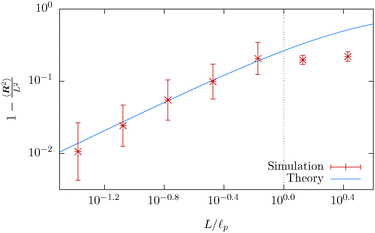 | ||
Fig. 9 The mean squared end-to-end distance 〈R2〉 as a function of the contour length L of the polymer plotted on a logarithmic scale, obtained from the simulation of a single free polymer. Each point represents an ergodic average (33) over the timespan of 1 s. The simulated mean squared end-to-end distance fits the theoretical prediction, given by (25) for short lengths of polymers, well. The deviation from the theoretical prediction for polymers longer than the persistence length L > ![[small script l]](https://www.rsc.org/images/entities/char_e146.gif) p is caused by the increase in the relaxation time, as can be seen in Fig. 10. The vertical dotted line denotes the upper bound of the fitting range, which corresponds to the situation, where the contour length equals the persistence length. p is caused by the increase in the relaxation time, as can be seen in Fig. 10. The vertical dotted line denotes the upper bound of the fitting range, which corresponds to the situation, where the contour length equals the persistence length. | ||
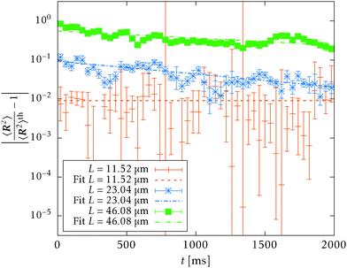 | ||
| Fig. 10 Relaxation of the mean squared end-to-end distance towards its theoretical equilibrium value 〈R2〉th on a semi-logarithmic scale. Each point represents an ergodic average (33) over the timespan of 50 ms. Estimated relaxation times from linear fits of the simulation data of a single polymer on the full interval are τr(23.04 μm) = 3.03 ± 0.35 s, τr(46.08 μm) = 5.51 ± 0.81 s which are exceeding the total simulation time. The shortest polymer's relaxation time estimate is overweighted by its error estimate, τr(11.52 μm) = 2.5 × 10⁴ ± 4.9 × 10⁷ s, which suggests that the polymer is already thermalised. | ||
This issue is not caused by the simulation method itself, but rather by the system we have chosen for this demonstration. For polymers much longer than their persistence length L ≫ ![[small script l]](https://www.rsc.org/images/entities/char_e146.gif) p, the bending stiffness does not constrain possible configurations of the polymer, which means that the Rouse model represents a suitable approximation. On the other hand, polymers much shorter than the persistence length L ≪
p, the bending stiffness does not constrain possible configurations of the polymer, which means that the Rouse model represents a suitable approximation. On the other hand, polymers much shorter than the persistence length L ≪ ![[small script l]](https://www.rsc.org/images/entities/char_e146.gif) p can be approximated by stiff rods. During the thermalisation, various sections of the polymers need to reorient themselves and thus the relaxation time associated with the thermalisation will follow the behaviour of the rotational relaxation time, which oscillates between the Rouse model and a stiff rod depending on the contour length L in question. It is known that the rotational relaxation time of the Rouse model is proportional to the square of the contour length L2, cf. Doi and Edwards,2 while for the stiff rod model the rotational relaxation time τr(29) is proportional to L3/ln
p can be approximated by stiff rods. During the thermalisation, various sections of the polymers need to reorient themselves and thus the relaxation time associated with the thermalisation will follow the behaviour of the rotational relaxation time, which oscillates between the Rouse model and a stiff rod depending on the contour length L in question. It is known that the rotational relaxation time of the Rouse model is proportional to the square of the contour length L2, cf. Doi and Edwards,2 while for the stiff rod model the rotational relaxation time τr(29) is proportional to L3/ln![[thin space (1/6-em)]](https://www.rsc.org/images/entities/char_2009.gif) L. Notice that the relaxation time scales at best quadratically L2 with the contour length independently of the discretisation and the persistence length. Hence, if we choose a different system with a smaller persistence length, we may be able to overcome this issue by decreasing the contour length of the polymer while preserving the contour length to persistence length ratio L/
L. Notice that the relaxation time scales at best quadratically L2 with the contour length independently of the discretisation and the persistence length. Hence, if we choose a different system with a smaller persistence length, we may be able to overcome this issue by decreasing the contour length of the polymer while preserving the contour length to persistence length ratio L/![[small script l]](https://www.rsc.org/images/entities/char_e146.gif) p. Indeed, if we choose DNA§ instead of F-actin we are able to thermalise, within the simulation environment, polymers longer than the persistence length, see Fig. 11, and confirm a good agreement between the theoretical prediction for WLC and our simulations. We note here that the difficulties with simulations of the F-actin polymers longer than persistence length do not present a problem in studying real-life system, as the typical length of the F-actin polymer does not typically exceed 1 μm, cf. Biron and Moses,46 and even in highly controlled environments, it rarely exceed its persistence length.41,47,48
p. Indeed, if we choose DNA§ instead of F-actin we are able to thermalise, within the simulation environment, polymers longer than the persistence length, see Fig. 11, and confirm a good agreement between the theoretical prediction for WLC and our simulations. We note here that the difficulties with simulations of the F-actin polymers longer than persistence length do not present a problem in studying real-life system, as the typical length of the F-actin polymer does not typically exceed 1 μm, cf. Biron and Moses,46 and even in highly controlled environments, it rarely exceed its persistence length.41,47,48
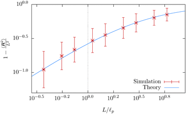 | ||
| Fig. 11 The mean squared end-to-end distance 〈R2〉 as a function of the contour length L of the polymer plotted on a logarithmic scale, obtained from the simulation of a single free DNA. Each point represents an ergodic average (33) over the timespan of 1 s. The simulated mean squared end-to-end distance fits the theoretical prediction, given by (25) for short lengths of polymers, well. The vertical dotted line denotes the contour length equal to the persistence length. | ||
5.4 Single polymer under tension
Another simulation set-up is to have a single long polymer under tension, L = 23.04 μm. In particular the initial set-up of the simulation is the same as in the previous case, i.e. a straight polymer with segments lengths equal to equilibrium value![[small script l]](https://www.rsc.org/images/entities/char_e146.gif) 0 and the viscosity also decreased to η = 1.71 × 10⁻⁴ pN μs nm−2. The polymer is then allowed to relax towards the thermal equilibrium for 10 s while constant anti-parallel forces are applied at both ends of the polymer, see Fig. 12. Estimates of the mean values of various equilibrium quantities are then again achieved by averaging over snapshots that are 1 ms apart over the time interval of 5 s from the initial time ti = 10 s, for reference see the ergodic average in the context of the mean squared end-to-end distance (33).
0 and the viscosity also decreased to η = 1.71 × 10⁻⁴ pN μs nm−2. The polymer is then allowed to relax towards the thermal equilibrium for 10 s while constant anti-parallel forces are applied at both ends of the polymer, see Fig. 12. Estimates of the mean values of various equilibrium quantities are then again achieved by averaging over snapshots that are 1 ms apart over the time interval of 5 s from the initial time ti = 10 s, for reference see the ergodic average in the context of the mean squared end-to-end distance (33).
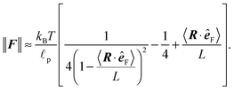
The relevant quantity in this case is the projected end-to-end vector R in the direction of the force êF, in this context called “extension”, which for the WLC can be related to the magnitude of the applied force ∥F∥, by an approximate relation1,5,35,45,49
 | (34) |
 | (35) |
Theoretical predictions (34) and (35) are compared with the simulation data in Fig. 13 and 14. The error bars in Fig. 13 denote the fluctuations in the end-to-end distance of the polymer, which are caused by thermal forces bending the polymer. Bending becomes increasingly difficult when larger forces are applied and indeed we see diminishing fluctuations when the pulling force is increased. Using (34) we can determine the actual persistence length ![[small script l]](https://www.rsc.org/images/entities/char_e146.gif) estp = 16.38 ± 0.77 μm, which is in good agreement with the value from the set-up of the model
estp = 16.38 ± 0.77 μm, which is in good agreement with the value from the set-up of the model ![[small script l]](https://www.rsc.org/images/entities/char_e146.gif) p = 17.2 μm. The estimate for the persistence length is obtained by the standard χ2 fitting method limited to the range 〈R·êF〉/L < 0.99, denoted by the dotted vertical line in Fig. 13. In order to demonstrate the transition between the two regimes of the polymer, we introduce an effective spring constant keff of the polymer defined as
p = 17.2 μm. The estimate for the persistence length is obtained by the standard χ2 fitting method limited to the range 〈R·êF〉/L < 0.99, denoted by the dotted vertical line in Fig. 13. In order to demonstrate the transition between the two regimes of the polymer, we introduce an effective spring constant keff of the polymer defined as
 | (36) |
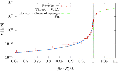 | ||
Fig. 13 The force magnitude ∥F∥ as a function of the relative extension 〈R·êF〉/L from a simulation of a single polymer under tension with contour length L = 23.04 μm. Each point corresponds to an ergodic average over the timespan of 5 s. Simulation results are compared with the theoretical predictions (34), (35) and for small relative length 〈êF·R〉 < L also fitted with (34) in order to obtain actual persistence length estimate. The black solid vertical line corresponds to the straight configuration 〈R·êF〉 = L, i.e. the initial configuration. The estimated persistence length ![[small script l]](https://www.rsc.org/images/entities/char_e146.gif) estp = 16.38 ± 0.77 μm is in good agreement with the actual value estp = 16.38 ± 0.77 μm is in good agreement with the actual value ![[small script l]](https://www.rsc.org/images/entities/char_e146.gif) p = 17.2 μm, see Table 2. The dotted vertical line denote the upper bound of the ranges for fitting of the parameters listed above. p = 17.2 μm, see Table 2. The dotted vertical line denote the upper bound of the ranges for fitting of the parameters listed above. | ||
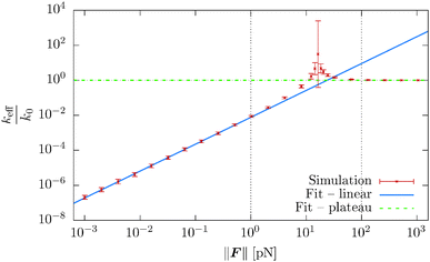 | ||
Fig. 14 The effective spring constant keff of the polymer, relative to the limiting value for large force magnitudes  , as a function of force magnitude F from the simulation of a single polymer under tension with the total polymer length L = 23.04 μm. Each point corresponds to ergodic average over the timespan of 5 s. In the small ∥F∥ regime the actual exponent for the effective spring constant keff ∝ ∥F∥ξ was determined to be ξ = 1.534 ± 0.0074 which is in good agreement with the theoretical value , as a function of force magnitude F from the simulation of a single polymer under tension with the total polymer length L = 23.04 μm. Each point corresponds to ergodic average over the timespan of 5 s. In the small ∥F∥ regime the actual exponent for the effective spring constant keff ∝ ∥F∥ξ was determined to be ξ = 1.534 ± 0.0074 which is in good agreement with the theoretical value  , see (38). In the high ∥F∥ regime the ratio between the theoretical value (37) and effective spring constant is keff/k0 = 1.0004 ± 0.0038. The crossover estimated from the intersection of the two linear fits is estimated to be ∥Fcross∥ = 23.93 ± 0.55 pN. The dotted vertical lines denote the ranges for fitting of the parameters listed above. , see (38). In the high ∥F∥ regime the ratio between the theoretical value (37) and effective spring constant is keff/k0 = 1.0004 ± 0.0038. The crossover estimated from the intersection of the two linear fits is estimated to be ∥Fcross∥ = 23.93 ± 0.55 pN. The dotted vertical lines denote the ranges for fitting of the parameters listed above. | ||
Let us note that such an effective spring constant diverges at 〈R·êF〉 = L, because we have chosen the straight configuration as the equilibrium value of such an effective spring, which also corresponds to polymer's configuration in the zero temperature limit, T → 0 K. Although such choice is unphysical, it has its own merits in terms of well defined asymptotes for both small and large ∥F∥. The simulation results are presented in Fig. 14. For large forces the effective spring constant coincides with the effective spring constant for a chained harmonic oscillators (35), i.e.
 | (37) |
we can recover the asymptotic spring constant for small forces
 | (38) |
6 Relaxation dynamics towards thermal equilibrium
While in the previous set-ups we investigated the equilibrium properties of our model, in this section we aim to verify some aspects of the dynamics. The initial configuration of the system consist of 200 straight independent polymers of total length L = 23.04 μm with segment lengths equal to their equilibrium values![[small script l]](https://www.rsc.org/images/entities/char_e146.gif) 0. For each polymer one of its ends is trapped in a harmonic potential with spring constant ktrap = k. The relaxation in equilibrium is then observed on different time-scales with different time steps in the range Δt ∈ [10−4,10−2] μs.
0. For each polymer one of its ends is trapped in a harmonic potential with spring constant ktrap = k. The relaxation in equilibrium is then observed on different time-scales with different time steps in the range Δt ∈ [10−4,10−2] μs.
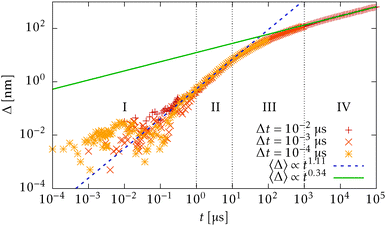
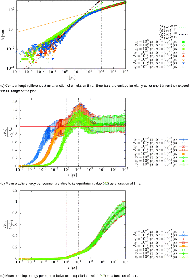
In Fig. 15 we plot the difference of the contour length from the initial configuration as a function of the total simulation time t on a log–log scale
| Δ = L − 〈R·êt=0〉 ∼ tξ, | (39) |
 for the WLC,50,51 which is experimentally verified in case of DNA.52
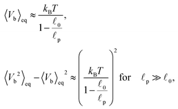
In order to understand the transition between those two relaxation regimes we investigate the mean energy stored in the bending (27) and elastic (7) potentials. To have some referential values we obtain analytical expressions for the mean value and variance of the bending and elastic potentials under the assumption that the associated degrees of freedom with those two potentials are decoupled and in thermal equilibrium. Furthermore we also consider neighbouring elements, i.e. nodes or segments, independent. The mean value of the bending energy (27) for a single joint is given by
 | (40) |
![[small script l]](https://www.rsc.org/images/entities/char_e146.gif) 0 is the segment's equilibrium length while its variance is
0 is the segment's equilibrium length while its variance is | (41) |
 . In our case x ≫ 1, cf.Table 2, hence we expand the mean value and the variance in x → ∞
where we are close to the regime where the equipartition theorem is valid. Similarly, the mean value of the elastic energy (7) for a single segment is
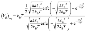 | (42) |
 determining the behaviour, which in our case is y ≫ 1. Consequently the variance is given by
Hence, we can again expand the exact results up to the leading order and obtain
for
 , which again shows that we are close to the regime where the equipartition theorem is valid. The total mean energies for a single polymers are then obtained by multiplying with the number of nodes or segments in the polymer as we assume they are independent.
Now we compare the theoretical equilibrium values with those obtained from the simulation during the relaxation. In Fig. 16 we observe that the elastic energy first relaxes towards thermal equilibrium (region I) with a relaxation time comparable to the relaxation time of a single segment τ![[small script l]](https://www.rsc.org/images/entities/char_e146.gif) . The unfreezing of transversal modes denoted by an increase of a mean bending energy 〈Vb〉 initially causes an increase in the mean elastic energy over the expected equilibrium value (40) (region II). The reason for such behaviour in a straight configuration is that every bending event also causes stretching of the involved segments. At the same time, the straight configuration also prevents these perturbations to relax locally as a consequence of applied constraints (21). At later times, when the polymer departs from the straight configuration, the influence of constraints is weakened and transversal modes are decoupled from longitudinal modes, which can be seen by the return of the mean elastic energy to its equilibrium value (40) (region III). By comparing Fig. 15 with Fig. 16, we hypothesize that the increase in the power law exponent above the theoretical prediction
. The unfreezing of transversal modes denoted by an increase of a mean bending energy 〈Vb〉 initially causes an increase in the mean elastic energy over the expected equilibrium value (40) (region II). The reason for such behaviour in a straight configuration is that every bending event also causes stretching of the involved segments. At the same time, the straight configuration also prevents these perturbations to relax locally as a consequence of applied constraints (21). At later times, when the polymer departs from the straight configuration, the influence of constraints is weakened and transversal modes are decoupled from longitudinal modes, which can be seen by the return of the mean elastic energy to its equilibrium value (40) (region III). By comparing Fig. 15 with Fig. 16, we hypothesize that the increase in the power law exponent above the theoretical prediction  is caused by a coupling of transversal and longitudinal modes leading to the “cooperative” regime. This goes against the assumption of their independence, hence invalidating the theoretical predictions in this regime provided by Hallatschek et al.50,51 When those modes decouple further relaxation towards the equilibrium is governed solely by bending properties of the polymer (region IV) and hence reproduces the theoretical value of the power law exponent for the WLC. In order to verify theoretical predictions (40), (41) we compare the total mean elastic energy obtained from the simulation for Δt = 10−2 μs, which is 〈Eb〉 = 34.2 ± 6.2kBT. This is in reasonable agreement with the theoretical prediction 〈Eb〉eq = 32.0 ± 5.7kBT, where the difference may be caused by the fact that transversal and longitudinal modes never truly decouple and that individual segments are not independent.
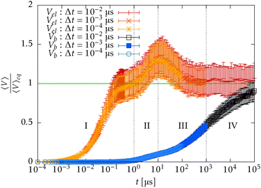 | ||
| Fig. 16 Mean bending and elastic energies per polymer relative to their equilibrium values as a function of time, obtained from (40), (42), based on the simulation of 200 independent polymers initially in the straight configuration of total length L = 23.04 μm with one end fixed in a harmonic potential with spring constant ktrap = k, while the other end is free to diffuse. Several simulations with time steps chosen in the range Δt ∈ [10−4,10−2] μs are evaluated in order to examine the behaviour in the wide range of time scales. We observe that the cooperative regime (region II) corresponds to the time interval where longitudinal modes are already equilibrated while transversal modes are just starting to equilibrate, hence causing additional perturbations to the segment length and increasing the mean elastic energy above its equilibrium value. The uncoupled regime (region IV) then corresponds to the situation where transversal modes are equilibrating while the longitudinal modes are already decoupled with the transversal modes as the elastic energy is again close to its equilibrium value. Fitting ranges for ξ are again denoted by vertical dotted lines. | ||
In order to further verify this hypothesis we inspect the dependency of such behaviour on the relaxation time of the longitudinal deformations of a single segment τ![[small script l]](https://www.rsc.org/images/entities/char_e146.gif) , see Fig. 17. As can be seen in Fig. 17b the position of the peak in the mean elastic energy 〈Vel〉, i.e. transition between regions II and III in Fig. 15 and 16, is independent of the relaxation time τ
, see Fig. 17. As can be seen in Fig. 17b the position of the peak in the mean elastic energy 〈Vel〉, i.e. transition between regions II and III in Fig. 15 and 16, is independent of the relaxation time τ![[small script l]](https://www.rsc.org/images/entities/char_e146.gif) and corresponds to the increase of the mean bending energy, cf.Fig. 17c. This suggests that the position of the peak is determined solely by the dynamics of the transversal modes. The power law exponent in the cooperative regime also depends on the relaxation time τ
and corresponds to the increase of the mean bending energy, cf.Fig. 17c. This suggests that the position of the peak is determined solely by the dynamics of the transversal modes. The power law exponent in the cooperative regime also depends on the relaxation time τ![[small script l]](https://www.rsc.org/images/entities/char_e146.gif) as can be seen in the Fig. 17a, namely ξ(τ
as can be seen in the Fig. 17a, namely ξ(τ![[small script l]](https://www.rsc.org/images/entities/char_e146.gif) = 10−2 μs) = 1.178 ± 0.014, ξ(τ
= 10−2 μs) = 1.178 ± 0.014, ξ(τ![[small script l]](https://www.rsc.org/images/entities/char_e146.gif) = 10−1 μs) = 1.114 ± 0.010, ξ(τ
= 10−1 μs) = 1.114 ± 0.010, ξ(τ![[small script l]](https://www.rsc.org/images/entities/char_e146.gif) = 10 μs) = 0.8941 ± 0.0078, while the behaviour in the decoupled regime is mostly unchanged ξ(τ
= 10 μs) = 0.8941 ± 0.0078, while the behaviour in the decoupled regime is mostly unchanged ξ(τ![[small script l]](https://www.rsc.org/images/entities/char_e146.gif) = 10−2 μs) = 0.3494 ± 0.0029, ξ(τ
= 10−2 μs) = 0.3494 ± 0.0029, ξ(τ![[small script l]](https://www.rsc.org/images/entities/char_e146.gif) = 10−1 μs) = 0.3436 ± 0.0030, ξ(τ
= 10−1 μs) = 0.3436 ± 0.0030, ξ(τ![[small script l]](https://www.rsc.org/images/entities/char_e146.gif) = 10 μs) = 0.3313 ± 0.0032. Notice also the large change in the behaviour when τ
= 10 μs) = 0.3313 ± 0.0032. Notice also the large change in the behaviour when τ![[small script l]](https://www.rsc.org/images/entities/char_e146.gif) = 1 μs, which is close to the typical time-scale where transversal modes unfreeze, Fig. 17c.
= 1 μs, which is close to the typical time-scale where transversal modes unfreeze, Fig. 17c.
On the other hand, if the relaxation time τ![[small script l]](https://www.rsc.org/images/entities/char_e146.gif) gets bigger than the characteristic time of the transversal modes, the behaviour of the system changes completely, see Fig. 18. As the longitudinal modes do not dissipate the energy fast enough they invalidate the assumption that these modes are independent and hence rise to a value much higher than the one estimated by (42), see Fig. 18c. The times where the mean elastic energy 〈Vel〉 saturates correspond to the moment of transition in the dynamics of the relaxation, as can bee seen in Fig. 18a. However, the power law exponent ξ no longer agrees with the theoretical prediction for the WLC
gets bigger than the characteristic time of the transversal modes, the behaviour of the system changes completely, see Fig. 18. As the longitudinal modes do not dissipate the energy fast enough they invalidate the assumption that these modes are independent and hence rise to a value much higher than the one estimated by (42), see Fig. 18c. The times where the mean elastic energy 〈Vel〉 saturates correspond to the moment of transition in the dynamics of the relaxation, as can bee seen in Fig. 18a. However, the power law exponent ξ no longer agrees with the theoretical prediction for the WLC  . Moreover the saturation of longitudinal modes also denotes the rapid increase in the mean bending energy, Fig. 18c.
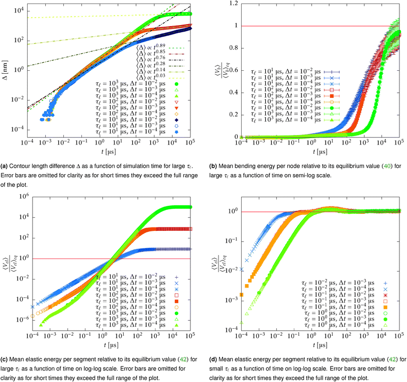 | ||
Fig. 18 The behaviour of the system when the relaxation time of a single segment length τ![[small script l]](https://www.rsc.org/images/entities/char_e146.gif) is larger than the characteristic time of the transversal modes deviates, even in long time asymptotic, from theoretical prediction for the WLC, see (a), where the power law exponent ξ strongly depends on τ is larger than the characteristic time of the transversal modes deviates, even in long time asymptotic, from theoretical prediction for the WLC, see (a), where the power law exponent ξ strongly depends on τ![[small script l]](https://www.rsc.org/images/entities/char_e146.gif) . The difference in the behaviour is even more pronounced in the time evolution of the mean bending energy, (b), which now depends on the relaxation time τ . The difference in the behaviour is even more pronounced in the time evolution of the mean bending energy, (b), which now depends on the relaxation time τ![[small script l]](https://www.rsc.org/images/entities/char_e146.gif) in contrast to Fig. 17c. Moreover, the mean value of the elastic energy no longer converges to its equilibrium value as can be seen in (c), which is in contrast with the behaviour for small τ in contrast to Fig. 17c. Moreover, the mean value of the elastic energy no longer converges to its equilibrium value as can be seen in (c), which is in contrast with the behaviour for small τ![[small script l]](https://www.rsc.org/images/entities/char_e146.gif) , see (d). , see (d). | ||
Possible experimental verification
The independence of the observed behaviour on the actual value of the relaxation time of longitudinal deformations τ![[small script l]](https://www.rsc.org/images/entities/char_e146.gif) , which is the only free parameter of the simulation that is not related to any available experimental value, suggests the possibility of an experimental verification of this quantity. In order to verify the existence of the new “cooperative” regime presented in this work in the case of F-actin, one needs to achieve a time resolution less then 1 μs along with a space resolution of less than 0.1 nm at the same time. Even though experimental methods such as fluorescence microscopy, optical tweezers54,55 and fast scanning atomic force microscopy56,57 are capable of working with such a resolution, it still might be challenging as the relative extension Δ is obscured by the thermal noise. Hence, it will require a large amount of consecutive measurements to obtain a large enough statistical ensemble. Moreover has to be careful not to add large masses or volumes at the ends of the polymer, as this might drastically alter its behaviour.
, which is the only free parameter of the simulation that is not related to any available experimental value, suggests the possibility of an experimental verification of this quantity. In order to verify the existence of the new “cooperative” regime presented in this work in the case of F-actin, one needs to achieve a time resolution less then 1 μs along with a space resolution of less than 0.1 nm at the same time. Even though experimental methods such as fluorescence microscopy, optical tweezers54,55 and fast scanning atomic force microscopy56,57 are capable of working with such a resolution, it still might be challenging as the relative extension Δ is obscured by the thermal noise. Hence, it will require a large amount of consecutive measurements to obtain a large enough statistical ensemble. Moreover has to be careful not to add large masses or volumes at the ends of the polymer, as this might drastically alter its behaviour.
7 Conclusion
The aim of this work was to develop a coarse grained model for thin long stiff semi-flexible polymers, applicable to an environment with large external forces, e.g. the cytoskeleton. The model is based on deformable cylinders as basic building blocks and exploits the assumption of the high stiffness and thinness, i.e. the Young's modulus is high compared to the bending stiffness, hence the polymers rather bend than deform, and the diameter of the polymer is much smaller than its typical length and also than its persistence length. We have derived from first principles (1) the equations of motion for the cylinders' end points in the overdamped limit (14), which inherently preserve autocorrelations of the noise applied on the end points (16). This is one of the key differences between our model and bead-rod models,12,13 where the beads' displacements are uncorrelated similar to bead-spring models,1–4 or to the second kind of bead-rod models,4,15 where the displacements of beads on opposite sides of a single segment are correlated only in the direction of the segment's axis (17). Our description of the overdamped diffusion differs from standard approaches based on the balance of forces and moments17 by the presence of thermal “torque” (15), a correction naturally arising from the intrinsically non-homogeneous diffusion of a cylindrical segment. Let us stress here that the presented model, already at the level of independent cylinders, is well suited for studying the behaviour of active nematic particles, e.g. active swimmers at low Reynolds number.32,33The full model of the polymer is achieved by chaining independent cylindrical segments by constraints (21), which are included in terms of virtual forces, obtained as a solution of the eqn (24), and which induced virtual effective “torques”, and by prescribing the bending potential (27) representing the semi-flexibility, which is included in the equations of motion in terms of an effective “torque” (28). The advantage of the bending model presented in this paper, the prevention of anti-alignment of neighbouring segments in case large forces are applied, thus increasing the overall stability of the simulation, is another difference with traditional approaches. Namely in the cytoskeleton, myosin motors apply forces of magnitude ∥F∥ ∝ pN thus exceeding thermal fluctuations.11,12 Furthermore the same polymer model can be as well used as a basis for models of molecular motors like Myosin-II, because of their polymer-like nature.38 These aspects of our model in particular will be fully utilised in our future work.
The full model is summarized in Section 4 from where it can be seen that the model has a similar computational complexity to the traditional bead-spring model introduced by Montesi et al.15 The main benefit of our approach is not only in decreasing the number of elements used in simulation, but also in the possibility to increase the time step, mainly owing to the increased friction for larger elements, thus improving the overall performance of the model even more, see the discussion in Section 4.1. In Section 5.1 we have provided a specific comparison of the model presented in this paper with a traditional bead-spring model, where we have achieved a simulation speed-up of more than 3 orders of magnitude, for a single polymer in the extreme case of very long segments. Although this approach truly show its strength for long segments, we have demonstrated that using the presented approach can be beneficial even for segments, which are short relative to the persistence length ![[small script l]](https://www.rsc.org/images/entities/char_e146.gif) p. This suggests the applicability of the model to wide range of (bio-)polymeric systems.
p. This suggests the applicability of the model to wide range of (bio-)polymeric systems.
The proposed model very well recovers the equilibrium behaviour of the WLC as is presented in Section 4. Both the polymer's thermal equilibrium end-to-end distance without, see 5.3, and with an applied tension, see Section 5.4, are evaluated and compared with theoretical predictions.34,35 Testing of the dynamics is achieved by analysing the relaxation from the fully elongated state towards thermal equilibrium, see Section 6, where we have described a new “cooperative” regime for short times, which suggests that on short time scales the longitudinal and transversal modes are coupled. This constitutes our second main result. For longer times, when transversal and longitudinal modes decouple, we recover the theoretically predicted behaviour.50,51 The emergency of “cooperative” behaviour on short-time scales (t < 10 μs in case of actin filament) might manifest itself as a faster relaxation towards equilibrium after the applied stress on the polymer network is released. Consequently, the response to the action of a molecular motor might deviate from that of the ideal WLC, which can contribute to the dynamics of filopodia and lamellipodia. Hence, the methods studying the actin-myosin networks based on the rigid rod models4,10,15 might have to be re-evaluated. This will also be the subject of further studies.
A Time evolution of macroscopic degrees of freedom
Here we derive eqn (4) from (1) by using the ansatz (2). First notice that| d(xi − X) = (vi − V) dt = [ω × (xi − X) + (xi − X)λ] dt. | (43) |
| j = π(i) ⇔ xi − X = X − xj, |
 | (44) |
The equation of motion for the centre of mass is obtain by summing (44) over all i
The equation governing rotations is obtained by summation of the cross product between xi − X and dvi, i.e. , where as for dvi we use (44). By using the symmetries of a cylinder we obtain
The last equation, for stretching is then obtained by summation (xi − X)dvi,
If we insert xi − X = ri![[t with combining circumflex]](https://www.rsc.org/images/entities/b_i_char_0074_0302.gif) and (3) and denote
and (3) and denote
Although the noises present in this set of equations  are in general correlated as
Because of the symmetries of the cylinder,  , we can conclude that they are in fact independent. The last step in order to obtain eqn (4) is noticing, that ω·
![[t with combining circumflex]](https://www.rsc.org/images/entities/b_i_char_0074_0302.gif) = 0.
= 0.
The remaining set of eqn (5) follow. The time evolution of the length is obtained from
![[small script l]](https://www.rsc.org/images/entities/char_e146.gif)
![[t with combining circumflex]](https://www.rsc.org/images/entities/b_i_char_0074_0302.gif) , and where we have also used (43). Similarly the orientation
, and where we have also used (43). Similarly the orientation ![[t with combining circumflex]](https://www.rsc.org/images/entities/b_i_char_0074_0302.gif) is governed by
is governed byB Equivalence of Smoluchowski and Langevin equations
Here we show how to obtain a Smoluchowski equation from a set of coupled Langevin equations in the case of an inhomogeneous environment by using the Itô calculus.18,25,58,59 We restrict ourselves to the set of Langevin equations of the following shape| dX± (t,W(α),W(β)) = A±(X+,X−) dt + B(X+,X−)·dW(α) ± C(X+,X−)·dW(β), | (45) |
We express the joint probability distribution μ(x+,x−) as the mean value over all the possible realisations of Wiener processes starting from arbitrary initial condition at time t = 0
| μt(x+,x−) = 〈δ(x+ − X+(t,W(α),W(β)))δ(x− − X−(t,W(α),W(β)))〉. |
The Smoluchowski equation then corresponds to the expression for time derivative of the joint probability distribution. In our case the only time dependent quantities in the mean value are random variables for the positions X±, which depends on time explicitly as well as via the realization of Wiener processes W. By using an Itô chain rule for the derivative we obtain
| ∂tX± = A±(X+,X−), |
| ∇W(α)X± = B(X+,X−), |
| ∇W(β)X± = ±C(X+,X−). |
In order to evaluate these expressions we exploit the fact that we have a Dirac δ-function present in the expression, e.g.
| 〈A+(X+,X−)·∇+δ(x+ − X+)δ(x− − X−)〉 = ∇+·〈A+(X+,X−)δ(x+ − X+)δ(x− − X−)〉 = ∇+·[A+(x+,x−)〈δ(x+ − X+)δ(x− − X−)〉] = ∇+·[A+(x+,x−)μt(x+,x−)]. |
By applying those rules on all terms we obtain the Smoluchowski equation
Hence we have found the one to one correspondence between the Langevin and Smoluchowski equation.
C Overdamped limit
Here we review the main results of the procedure for time-scale separation described by Pešek24 and apply it to obtain a Smoluchowski equation from a Fokker–Planck equation.C.1 General framework
The procedure is based on a couple of assumptions. The first one is that we can decompose the time evolution of the joint probability distribution to one part describing the evolution of the fast degrees of freedom and another for the slow degrees of freedom. Furthermore it assumes that the time evolution is dominated by the dynamics of the fast degrees of freedom and that the evolution of slow degrees of freedom can be considered as a perturbation, | (46) |
 denotes the part of the backward Kolmogorov generator corresponding to the time evolution of the fast degrees of freedom, where we explicitly introduce the degree of time scale separation ε, and
 ![[script L]](https://www.rsc.org/images/entities/char_e144.gif) S* is the part corresponding to the slow degrees of freedom. The last assumption is that given the particular configuration of slow degrees of freedom xS the backward Kolmogorov generator for fast degrees of freedom
S* is the part corresponding to the slow degrees of freedom. The last assumption is that given the particular configuration of slow degrees of freedom xS the backward Kolmogorov generator for fast degrees of freedom  has a unique steady state distribution ρ(xF|xS), to which every initial configuration of fast degrees of freedom converges
 | (47) |
Under these conditions it can be shown24 that the time evolution of the joint probability distribution up to the first power in ε is fully determined by the marginal distribution of the slow degrees of freedom
Namely
 is the Drazin pseudo inverse|| of
  , see Drazin,60 and λi/ε are non-zero eigenvalues of
  . Hence the dynamics for slow degrees of freedom is autonomous and Markovian up to the first order in degree of time scale separation ε and can be described by
 | (48) |
 and much smaller than the characteristic time of the slow degrees of freedom τS, τF ≪ Δt ≪ τS. Moreover the joint probability distribution is at any time given by
| μt(xF,xS) = νt(xS)ρ(xF|xS) + εΔμt(xF,xS) + O(ε2Δt,Δt2), |
 | (49) |
In the case of the overdamped limit we expect that velocities, or in phase space formalism canonical momenta, relax towards equilibrium much faster than positions, hence they will represent the fast degrees of freedom while the positions corresponds to the slow degrees of freedom. Following the general procedure, the first step is obtaining the canonical momenta p± associated with the positions of the cylinders' end points x±. Then we will provide a time evolution equation for the joint probability distribution μ(x+,x−,p+,p−;t) where we will identify the time evolution of the fast degrees of freedom. And in the end we derive an autonomic time evolution eqn (48) for the marginal probability distribution ν(x+,x−;t), for which we later find the corresponding Langevin equations. In the process we also obtain an estimate for relaxation time of the fast degrees of freedom τF as well as the correction to the joint probability distribution (49).
C.2 Canonical momentum
Under the assumption that the external forces applied on the segment don't depend on velocities, no presence of magnetic fields is assumed, the only part of the Langrangian that does depend on velocities is the kinetic energy given bywhere we again used the symmetries of the cylinder, i.e. all terms odd in xi − X are inherently zero. The kinetic energy can also equivalently be expressed in terms of the velocities of the end points
As the kinetic energy is the only part of the Lagrangian that depends on velocities, we have all the information necessary in order to derive canonical momenta
Notice that for pure translation both moments are the same and correspond to the moment of a point particle with the same mass and velocity, however for pure rotations they have an opposite sign and the same magnitude, corresponding to the angular momentum of the segment divided by its length. It is also valid that
Having canonical momenta we derive the kinetic part of the Hamiltonian
The time evolution of canonical momenta is then given by
C.3 Time evolution of probability density
After successful determination of the canonical momenta it is time to investigate the time evolution of the joint probability evolution. First we use a technique similar to the one described in Appendix B in order to obtain the Fokker–Planck equation for the full systemHere we identify the time evolution of the fast degrees of freedom p± as a part of the full generator, which ensures the thermalisation of the momenta,
Indeed there exists an unique stationary solution  , which is given by the Boltzmann distribution
hence, as we can always decompose any probability distribution to the marginal distribution of positions and conditional distribution of momenta, the generator also obeys the last necessary condition (47). Remaining terms in the Fokker–Planck equation then correspond to the time evolution of slow degrees of freedom
As we have shown the given decomposition obeys all necessary requirements. We can proceed to evaluate all terms in the effective time-evolution for the slow degrees of freedom (48). The first term is determined by
 | (50) |
We can see that there is no zeroth order contribution, which is to be expected as the zeroth order corresponds to the ballistic motion.
In order to proceed further we have to investigate the behaviour of the generator for the fast degrees of freedom  for terms linear in the canonical momentum. Moreover all the terms appearing in (50) can be rewritten in terms of p+ ± p−, see
The pseudo inverse is just given by the matrix inverse
From those expressions we can easily determine relevant relaxation times
 | (51) |
The next step corresponds to the determination of the term
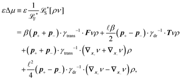 | (52) |
The last step is then the application of (50) on (52) and integrating over the canonical momenta p±, where we will use
From the probability distribution (52) we can also directly obtain the mean canonical momenta conditioned on the positions x±
The Smoluchowski eqn (13) then coincides with the continuity equation for probability densities
| ∂νt +∇+·jν+ + ∇−·jν− = 0. |
D Time-step constraints
When dealing with numerical simulations, one usually wants to have the simulation time step as large as possible. However in order for the simulation to be stable and reasonably precise there are certain limits to how large the time step can be. In this appendix we will provide some estimates on the upper bound of the time step, only from the stability point of view. Additional constraints, taking into account precision issues of the simulation, will depend on the physical properties of interest, e.g. relaxation times for relevant quantities.D.1 Spatial resolution of diffusion
The first constraint comes from the fact that we want to restrict the possibility of two segments to pass through each other in a single iteration without interacting. The main limiting dimension in our case it the width of the polymer, which leads to a constraint for the maximal displacement of the end-points in one single time step Δx±| 2∥Δx±∥ < d, | (53) |
Translations: the translational diffusion is described by eqn (14)
As we can see, the displacement is determined by the realisation of the Wiener process over a finite time interval, which is unfortunately unbound, hence the constraint (53) in its naive version can in principle not be applied. Instead we determine the confidence interval in which the displacement Δx± will not be bigger than the diameter of the segment d in terms of multiples of the variance of the Wiener process cσ, i.e. 1σ confidence interval corresponds to cσ = 1, 2σ corresponds to cσ = 2, etc. Then the constraint (53) is replaced by
 | (54) |
which yields to following constraint
or in terms of the constraint on the time step
 | (55) |
where the maximum is taken over eigenvalues. This finally leads to the constraint on the time step
 | (56) |
D.2 Longitudinal stiffness
Another cause of instability can be the longitudinal extension. When a fluctuation occurs in the length of the segment, the elastic effective “torque” (8) tries to correct such fluctuation. This leads to a condition on the induced length correction Δ![[small script l]](https://www.rsc.org/images/entities/char_e146.gif) , which has to be (much) smaller than twice the original fluctuation Δ
, which has to be (much) smaller than twice the original fluctuation Δ![[small script l]](https://www.rsc.org/images/entities/char_e146.gif) 0. If this is not the case, the elastic forces will cause an oscillation with increasing amplitude. when neglecting the noise, the equation of motion for the segments length reads
0. If this is not the case, the elastic forces will cause an oscillation with increasing amplitude. when neglecting the noise, the equation of motion for the segments length readswhich after discretisation leads to the condition
By using the equilibrium length ![[small script l]](https://www.rsc.org/images/entities/char_e146.gif) 0 instead of the actual length
0 instead of the actual length ![[small script l]](https://www.rsc.org/images/entities/char_e146.gif) for the estimate and rewriting it as a condition for the time step Δt we obtain
for the estimate and rewriting it as a condition for the time step Δt we obtain
 | (57) |
D.3 Bending
The last possible cause of instability in our model can be the bending potential. The argument follows the train of thoughts presented in the discussion of the longitudinal stiffness, namely we start from the condition that the reaction has to be smaller than the initial perturbation. In the case of bending it corresponds to the following condition(1 − ![[t with combining circumflex]](https://www.rsc.org/images/entities/b_i_char_0074_0302.gif) i· i·![[t with combining circumflex]](https://www.rsc.org/images/entities/b_i_char_0074_0302.gif) i+1)after < (1 − i+1)after < (1 − ![[t with combining circumflex]](https://www.rsc.org/images/entities/b_i_char_0074_0302.gif) i· i·![[t with combining circumflex]](https://www.rsc.org/images/entities/b_i_char_0074_0302.gif) i+1)before, i+1)before, |
−Δ![[t with combining circumflex]](https://www.rsc.org/images/entities/b_i_char_0074_0302.gif) i·Δ i·Δ![[t with combining circumflex]](https://www.rsc.org/images/entities/b_i_char_0074_0302.gif) i+1 < Δ i+1 < Δ![[t with combining circumflex]](https://www.rsc.org/images/entities/b_i_char_0074_0302.gif) i· i·![[t with combining circumflex]](https://www.rsc.org/images/entities/b_i_char_0074_0302.gif) i+1 + i+1 + ![[t with combining circumflex]](https://www.rsc.org/images/entities/b_i_char_0074_0302.gif) i·Δ i·Δ![[t with combining circumflex]](https://www.rsc.org/images/entities/b_i_char_0074_0302.gif) i+1. i+1. |
The differential equation for tangent vector can be again obtained from equation of motion (14) and reads
where a is the bending stiffness a =
![[small script l]](https://www.rsc.org/images/entities/char_e146.gif) pkBT. After substitution in the condition we obtain
pkBT. After substitution in the condition we obtainwhich under the approximations of
![[t with combining circumflex]](https://www.rsc.org/images/entities/b_i_char_0074_0302.gif) i·
i·![[t with combining circumflex]](https://www.rsc.org/images/entities/b_i_char_0074_0302.gif) i+1 ≈ 1 and
i+1 ≈ 1 and ![[small script l]](https://www.rsc.org/images/entities/char_e146.gif) =
= ![[small script l]](https://www.rsc.org/images/entities/char_e146.gif) 0 simplifies to
0 simplifies to | (58) |
D.4 Bead-spring model
Similar estimates can be obtained for the bead-spring model. Here we just provide the results without derivation as it is analogous to the more complicated case of stiff cylinders.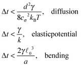 | (59) |
![[small script l]](https://www.rsc.org/images/entities/char_e146.gif) 0 denotes the equilibrium distance between the centres of the beads, which has to satisfy
0 denotes the equilibrium distance between the centres of the beads, which has to satisfy ![[small script l]](https://www.rsc.org/images/entities/char_e146.gif) 0 < 2d in order to avoid the possibility of two polymers passing through each other.
0 < 2d in order to avoid the possibility of two polymers passing through each other.
Acknowledgements
We acknowledge financial support from the Research Fund Flanders (FWO-Vlaanderen), Grant no. G0821.13. We are grateful to Enrico Carlon, Michiel Laleman and Karel Netočný for many useful discussions and suggestions. We are also grateful to Tim Odenthal and Simon Vanmaercke for their help with Mpacts toolbox and Ramesh Subramani for the discussion about experimental techniques.References
- S. S. Andrews, Phys. Biol., 2014, 11, 011001 CrossRef PubMed.
- M. Doi and S. Edwards, The Theory of Polymer Dynamics, Oxford University Press Inc., New York, 1986, p. 391 Search PubMed.
- P. T. Underhill and P. S. Doyle, J. Non-Newtonian Fluid Mech., 2004, 122, 3–31 CrossRef CAS.
- M. Somasi, B. Khomami, N. J. Woo, J. S. Hur and E. S. Shaqfeh, J. Non-Newtonian Fluid Mech., 2002, 108, 227–255 CrossRef CAS.
- S. M. Bhattacharjee, A. Giacometti and A. Maritan, J. Phys.: Condens. Matter, 2013, 25, 503101 CrossRef PubMed.
- R. M. Jendrejack, J. J. de Pablo and M. D. Graham, J. Chem. Phys., 2002, 116, 7752 CrossRef CAS.
- S. Mohammadinejad, R. Golestanian and H. Fazli, Soft Matter, 2012, 8, 3649 RSC.
- D. Panja, G. T. Barkema and J. M. J. van Leeuwen, Phys. Rev. E: Stat., Nonlinear, Soft Matter Phys., 2015, 92, 032603 CrossRef PubMed.
- B. Liu, J. Wang, X. Fan, Y. Kong and H. Gao, J. Comput. Phys., 2008, 227, 2794–2807 CrossRef CAS.
- C. H. Schreiber, M. Stewart and T. Duke, Proc. Natl. Acad. Sci. U. S. A., 2010, 107, 9141–9146 CrossRef CAS PubMed.
- A. D. Mehta, R. S. Rock, M. Rief, J. A. Spudich, M. S. Mooseker and R. E. Cheney, Nature, 1999, 400, 590–593 CrossRef CAS PubMed.
- D. Gordon, A. Bernheim-Groswasser, C. Keasar and O. Farago, Phys. Biol., 2012, 9, 026005 CrossRef PubMed.
- T. Kim, W. Hwang, H. Lee and R. D. Kamm, PLoS Comput. Biol., 2009, 5, e1000439 Search PubMed.
- P. Gutjahr, R. Lipowsky and J. Kierfeld, Europhys. Lett., 2006, 76, 994–1000 CrossRef CAS.
- A. Montesi, D. C. Morse and M. Pasquali, J. Chem. Phys., 2005, 122, 084903 CrossRef PubMed.
- J. McConnell, Rotational Brownian Motion and Dielectric Theory, Academic Press, London, 1980, p. 300 Search PubMed.
- J. K. R. Dhont, Soft matter: complex materials on mesoscopic scale, Jülich, 2002, p. 31 Search PubMed.
- B. Øksendal, Stochastic differential equations, Springer-Verlag, Heidelberg New York, 5th edn, 2003, p. 352 Search PubMed.
- G. Li and J. X. Tang, Phys. Rev. E: Stat., Nonlinear, Soft Matter Phys., 2004, 69, 1–5 Search PubMed.
- S. Broersma, J. Chem. Phys., 1960, 32, 1626 CrossRef CAS.
- S. Broersma, J. Chem. Phys., 1960, 32, 1632 CrossRef CAS.
- S. Broersma, J. Chem. Phys., 1981, 74, 6989–6990 CrossRef.
- M. Yang and M. Ripoll, Phys. Rev. E: Stat., Nonlinear, Soft Matter Phys., 2013, 87, 1–7 Search PubMed.
- J. Pešek, PhD thesis, Faculty of Mathematics and Physics, Charles University in Prague, 2013.
- N. G. van Kampen, J. Stat. Phys., 1981, 24, 175–187 CrossRef.
- N. G. van Kampen, J. Stat. Phys., 1981, 25, 431–442 CrossRef.
- N. G. van Kampen, Z. Phys. B: Condens. Matter, 1987, 68, 135–138 CrossRef.
- Y. Klimontovich, Phys. A, 1990, 163, 515–532 CrossRef.
- I. Sokolov, Chem. Phys., 2010, 375, 359–363 CrossRef CAS.
- O. Farago and N. Grønbech-Jensen, Phys. Rev. E: Stat., Nonlinear, Soft Matter Phys., 2014, 89, 013301 CrossRef PubMed.
- T. Vicsek, A. Czirók, E. Ben-Jacob, I. Cohen and O. Shochet, Phys. Rev. Lett., 1995, 75, 1226–1229 CrossRef CAS PubMed.
- T. Vicsek and A. Zafeiris, Phys. Rep., 2012, 517, 71–140 CrossRef.
- X.-q. Shi and Y.-q. Ma, Nat. Commun., 2013, 4, 3013 Search PubMed.
- L. D. Landau and E. M. Lifshitz, Statistical physics, Elsevier Ltd, Oxford, 3rd edn, 1980, p. 544 Search PubMed.
- J. F. Marko and E. D. Siggia, Macromolecules, 1995, 28, 8759–8770 CrossRef CAS.
- O. Kratky and G. Porod, Recl. Trav. Chim. Pays-Bas, 1949, 68, 1106–1122 CrossRef CAS.
- J. Kierfeld, P. Gutjahr, T. Kühne, P. Kraikivski and R. Lipowsky, J. Comput. Theor. Nanosci., 2006, 3, 898–911 CrossRef CAS.
- T. D. Pollard, J. Cell Biol., 1982, 95, 816–825 CrossRef CAS PubMed.
- S. Vanmaercke, B. Smeets and T. Odenthal, Mpacts webpage, 2015, http://mpacts.dem-research-group.com/index.html.
- O. N. Yogurtcu, J. S. Kim and S. X. Sun, Biophys. J., 2012, 103, 719–727 CrossRef CAS PubMed.
- H. Nagashima and S. Asakura, J. Mol. Biol., 1980, 136, 169–182 CrossRef CAS PubMed.
- F. Gittes, B. Mickey, J. Nettleton and J. Howard, J. Cell Biol., 1993, 120, 923–934 CrossRef CAS PubMed.
- H. Kojima, A. Ishijima and T. Yanagida, Proc. Natl. Acad. Sci. U. S. A., 1994, 91, 12962–12966 CrossRef CAS.
- T. Odijk, Macromolecules, 1995, 28, 7016–7018 CrossRef CAS.
- M. Wang, H. Yin, R. Landick, J. Gelles and S. Block, Biophys. J., 1997, 72, 1335–1346 CrossRef CAS PubMed.
- D. Biron and E. Moses, Biophys. J., 2004, 86, 3284–3290 CrossRef CAS PubMed.
- D. Sept, J. Xu, T. D. Pollard and J. Andrew McCammon, Biophys. J., 1999, 77, 2911–2919 CrossRef CAS PubMed.
- P. A. Kuhlman, Cell Motil. Cytoskeleton, 2005, 61, 1–8 CrossRef CAS PubMed.
- E. S. G. Shaqfeh, G. H. McKinley, N. Woo, D. A. Nguyen and T. Sridhar, J. Rheol., 2004, 48, 209 CrossRef CAS.
- O. Hallatschek, E. Frey and K. Kroy, Phys. Rev. E: Stat., Nonlinear, Soft Matter Phys., 2007, 75, 031905 CrossRef PubMed.
- O. Hallatschek, E. Frey and K. Kroy, Phys. Rev. E: Stat., Nonlinear, Soft Matter Phys., 2007, 75, 031906 CrossRef PubMed.
- O. Otto, S. Sturm, N. Laohakunakorn, U. F. Keyser and K. Kroy, Nat. Commun., 2013, 4, 1780 CrossRef PubMed.
- F. W. J. Olver, SIAM J. Math. Anal., 1991, 22, 1460–1474 CrossRef.
- K. S. Lee, H. Balci, H. Jia, T. M. Lohman and T. Ha, Nat. Commun., 2013, 4, 1878 CrossRef PubMed.
- I. Heller, G. Sitters, O. D. Broekmans, G. Farge, C. Menges, W. Wende, S. W. Hell, E. J. G. Peterman and G. J. L. Wuite, Nat. Methods, 2013, 10, 910–916 CrossRef CAS PubMed.
- N. Crampton, M. Yokokawa, D. T. F. Dryden, J. M. Edwardson, D. N. Rao, K. Takeyasu, S. H. Yoshimura and R. M. Henderson, Proc. Natl. Acad. Sci. U. S. A., 2007, 104, 12755–12760 CrossRef CAS PubMed.
- Y. Suzuki, N. Sakai, A. Yoshida, Y. Uekusa, A. Yagi, Y. Imaoka, S. Ito, K. Karaki and K. Takeyasu, Sci. Rep., 2013, 3, 1–7 Search PubMed.
- L. C. Evans, An Introduction to Stochastic Differential Equations, American Mathematical Society, 2013, p. 151 Search PubMed.
- W. Feller, An introduction to probability theory and its applications, Wiley, 3rd edn, 1968, vol. 1, p. 509 Search PubMed.
- M. P. Drazin, Am. Math. Monthly, 1958, 65, 506 CrossRef.
Footnotes |
| † Note that with simulation duration we mean the actual time that it takes to complete a simulation, while with simulation time we denote the time over which we simulate a system, i.e. number of iterations × Δt. |
‡ In the Table 3 we have used a more exact expression (59) for the maximal estimate on the time step based on the stability with respect to bending for the bead-spring model with ![[small script l]](https://www.rsc.org/images/entities/char_e146.gif) 0 = d. 0 = d. |
§ Properties of DNA are ![[small script l]](https://www.rsc.org/images/entities/char_e146.gif) p = 43.3 nm, d = 2 nm, cf. Odijk44 and Wang et al.,45 which implies p = 43.3 nm, d = 2 nm, cf. Odijk44 and Wang et al.,45 which implies ![[small script l]](https://www.rsc.org/images/entities/char_e146.gif) = 8 nm, Δt = 0.5 ns. = 8 nm, Δt = 0.5 ns. |
¶ Generalized exponential integral is defined as  . In case k = 0 the exponential integral reduces to E0(x) = e−x/x. Asymptotic behaviour was provided for example by Olver.53 . In case k = 0 the exponential integral reduces to E0(x) = e−x/x. Asymptotic behaviour was provided for example by Olver.53 |
|| It is a linear operator which maps an argument to its inverse whenever invertible and to 0 whenever it belongs to the kernel of  . . |
| This journal is © The Royal Society of Chemistry 2016 |

