
 Open Access Article
 This Open Access Article is licensed under a
 Creative Commons Attribution 3.0 Unported Licence
Self-assembly of three-dimensional ensembles of magnetic particles with laterally shifted dipoles
Arzu B.
Yener
and
Sabine H. L.
Klapp
*
Institute of Theoretical Physics, Technical University Berlin, Hardenbergstr. 36, 10625 Berlin, Germany. E-mail: klapp@physik.tu-berlin.de
First published on 8th January 2016
Abstract
We consider a model of colloidal spherical particles carrying a permanent dipole moment which is laterally shifted out of the particles' geometrical centres, i.e. the dipole vector is oriented perpendicular to the radius of the particles. Varying the shift δ from the centre, we analyse ground state structures for two, three and four hard spheres, using a simulated annealing procedure. We also compare earlier ground state results. We then consider a bulk system at finite temperatures and different densities. Using molecular dynamics simulations, we examine the equilibrium self-assembly properties for several shifts. Our results show that the shift of the dipole moment has a crucial impact on both the ground state configurations as well as the self-assembled structures at finite temperatures.
1 Introduction
Recent advances in particle synthesis and the permanent need for novel materials meeting more and more specialised requirements encourage the search for novel types of functionalized particles. Promising candidates in this area are colloids with directional interactions. These interactions are the key for the controlled self-assembly of colloidal particles into specific structures. Recent research on this topic resulted in complex colloidal particles characterised by the complex shape,1–3 anisotropic internal symmetry4,5 or surface charges.6,7 Understanding the interaction-induced behaviour of such particles is crucial for optimizing their application, e.g. in materials science biomedicine or sensing.Yet, not only the application of functionalized particles is of interest but also their capability to serve as model systems to study fundamental concepts of physics such as self-organization,8,9 chirality,2,10–12 synchronisation,8,13–15 critical phenomena,16,17 entropic effects18,19 and active motion,20,21 to name a few. A paradigm example is the model of dipolar hard and soft spheres which is a well-established model to examine and understand the properties of magnetic colloidal particles immersed in a solvent, also called ferrofluids. From numerous studies of the phase behavior of dipolar liquids (e.g.ref. 22 and 23), and especially of their structural properties (e.g.ref. 24 and 25), it is known that the dipoles assemble into chains, rings and branched structures at sufficiently large dipolar strengths and low densities.
Here, we focus on (permanent) ferromagnetic colloids with anisotropic symmetry, i.e. the magnetic moment within the colloidal particle is not located at the geometric centre of the particle. A first theoretical description for decentrally located dipoles was introduced by Holm et al.26–28 In their model, spherical particles carry a dipole moment which is shifted out of the particle centre and is oriented parallel to the radius vector of the particle. The model describes very well the cluster formation of particles carrying a magnetic cap.29 Yet, it is insufficient to mimic the self-assembly of so-called patchy colloids,9 that is, silicon balls carrying magnetic cubes beneath their surfaces. Furthermore, the model does not reproduce the zig-zag chained structures formed by magnetic Janus particles in an external field, i.e. particles in which one hemisphere of silica spheres is covered with a magnetic coat.8,30 The concept of shifting the dipole was later extended by fixing the amount of shift and varying the orientation of the dipole moment vector within the particle31 which was proven to be more convenient for patchy collids.
In the present contribution we consider a model in which the dipole moment is laterally shifted such that the radius vector and the dipole moment vector are oriented perpendicular. The same model was also proposed in ref. 31. However, here we fix the orientation of the dipole moment and vary the amount of shift. Thereby, we do not only aim at modeling synthesized particles mentioned above. Rather, we are interested in understanding the impact of successively shifting the dipole on the self-assembly of such particles. To this end, we perform ground state calculations for a small number of dipolar hard spheres and conduct Molecular Dynamics (MD) simulations to study the bulk at finite temperature in three dimensions (3D). Very recently, Novak et al. have considered the same model;32 however, they restricted their study to systems where the particles are fixed in a plane with freely rotating dipoles. Thus, they considered a quasi-two-dimensional (q2D) system. Besides, the authors examined the system at one fixed density. Here, we examine a three dimensional system of such particles at zero temperature and conduct MD simulations of the bulk at several thermodynamic state points. Thereby, we aim at quantitive characterization in which the shift is the state parameter in the system.
The remainder of the paper is structured as follows. In Section 2, we present the model and the equations of motion, Section 3 refers to the computational methods and Sections 4 and 5 include the results for the ground state calculations and for the structural analysis of the bulk systems, respectively. We close the paper by a summary and outlook.
2 Model and equations of motion
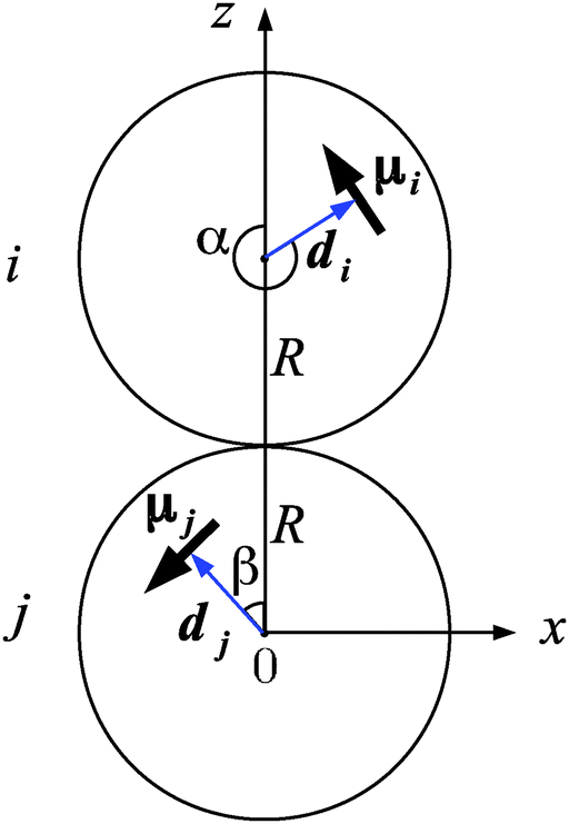
Our model consists of N spherical particles carrying a permanent dipole moment μi, (i = 1,…,N), which is laterally shifted with respect to the center of particles. A sketch is given in Fig. 1. In the body-fixed reference frame (in the following denoted by the subscript b), the location of μi is specified by the shift vector dbi = d(1,0,0), and its orientation is given by the vector μbi = μ(0,0,1), with d and μ being constants for all particles. Hence, di and μi are oriented perpendicular to one another. Thus, our particles differ from those considered in ref. 27 where di and μi are arranged parallel and hence μi is shifted radially.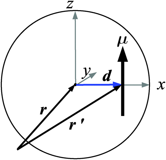 | ||
| Fig. 1 Sketch of a dipolar sphere with a laterally shifted dipole moment. Also shown are the axes of the body-fixed coordinate system. | ||
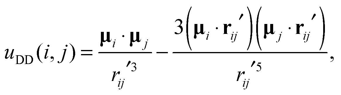
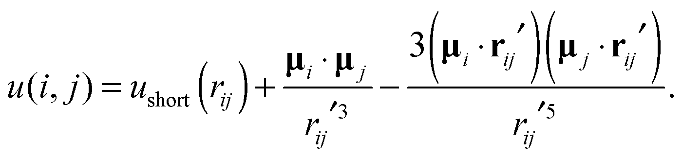
In the laboratory reference frame, ri is the position vector of the particle centre while the position vector of μi is given by ri′ = ri + di, where di now denotes the shift vector in the laboratory frame. For d = 0, ri′ coincides with ri yielding conventional dipolar systems with centered dipoles. A discussion of typical values of the relative shift δ = |d|/2|R| (where |R| is the particle radius) is given at the end of Section 5.1. The total pair potential between two particles i and j consists of a short-range repulsive potential, ushort(rij), and the dipole–dipole potential,
 | (1) |
 | (2) |
 | (3) |
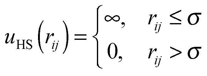
Second, for the ground-state calculations presented in Section 4, we set ushort(rij) equal to the hard sphere (HS) potential defined as
 | (4) |
 | (5) |
 | (6) |
 | (7) |
m![[r with combining umlaut]](https://www.rsc.org/images/entities/b_char_0072_0308.gif) i = Fi i = Fi | (8) |
 | (9) |
 | (10) |
![[Q with combining dot above]](https://www.rsc.org/images/entities/b_char_0051_0307.gif) i is the time derivative of the quaternion Qi = (q0i,q1i,q2i,q3i) which we employ to describe the orientation of the particle (specified in ref. 34). The matrix W is defined as (see ref. 34)
i is the time derivative of the quaternion Qi = (q0i,q1i,q2i,q3i) which we employ to describe the orientation of the particle (specified in ref. 34). The matrix W is defined as (see ref. 34)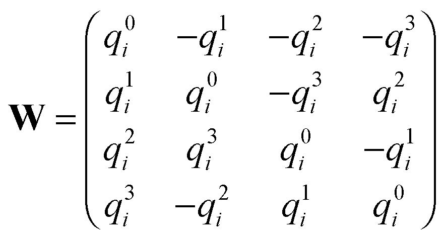 | (11) |
3 Computer simulations
3.1 Molecular dynamics simulations
In our MD simulations, we constrain the temperature to a constant value T by using a Gaussian isokinetic thermostat.34 Hence, the linear and angular momenta of the particles are rescaled by the factors and
and  , respectively, where
  (with ṙi = |dri/dt|) and
  (with ωi = |ωi|) are the translational and rotational kinetic temperatures of the system. Further, kB is the Boltzmann constant. We solve the corresponding isokinetic equations for translational and rotational motion using a Leapfrog algorithm, following the schemes suggested in ref. 34 and 35. To account for the long range dipolar interaction uDD, we apply the three-dimensional Ewald summation technique.33 Specifically, we use a cubic simulation box with side length Lx = Ly = Lz = L and employ periodic boundary conditions in a conducting surrounding. The parameter α which determines the convergence of the real space part of the Ewald sum is chosen to be α = 6.0/L which is large enough to consider only the central box with n = 0 in the real space. For the Fourier part of the Ewald sum we consider wave vectors k up to (k)2 = 54, giving a total number of wave vectors nk = 1500. In the MD simulations, we use the following reduced units: ρ* = σ3ρ, dipole moment
  , time
  and temperature T* = kBT/ε. The simulations were carried out with N = 864 particles and with a time step of Δt* = 0.0025. Typical simulations lasted for 3 × 10⁶ steps.
3.2 Simulated annealing
To investigate ground state configurations of small clusters of particles interacting via the pair potential u(i, j) = uHS + uDD [see eqn (1), (2) and (4)], we employ a simulated annealing procedure which involves a Monte Carlo simulation using the Metropolis algorithm.34 Within this method, we choose initial states with comparable dipolar and thermal energies, i.e. uDD/kBT ≈ 1. Here, uDD is the dipolar energy of two hard spheres in contact with central dipoles having head to tail orientation. We then lower the temperature stepwise to zero. At each temperature, 106 trial moves are performed while conducting the usual metropolis scheme involving translational and rotational trial moves. We realize an acceptance ratio of 60% by regularly adjusting the absolute value of the translational displacement during the simulation. New orientational configurations are generated by rotating the particles with a constant angle of dϕ = π/18 around one of the three axes of the laboratory fixed frame. In order to ensure that we reach the state with lowest energy, we start several simulations for each set of parameters and choose those results with the lowest energy as the minimum energy state.4 Ground state considerations
4.1 Ground state energies and configurations of two and three particles
As a first step towards understanding the impact of the lateral shift, we considered two hard spheres (N = 2) with shifted dipoles (see eqn (2) with ushort = uHS). This case has already been discussed in ref. 32. As a background for our later discussion of the case N > 2, we have rederived some key results such as the ground state energy and the corresponding pair configurations as a function of the relative shift δ. The results are summarized in the Appendix.The case of three particles was also considered in ref. 32. However, for very small and very high shifts, we find slightly different ground state energies and thus structures than those in ref. 32. Here, we discuss the main results and differences.
For three particles, shifting the dipole has the same effect on the ground state energies and configurations as for two particles. Thus, the former also rapidly decreases with increasing shift qualitatively in the same way as shown in Fig. 10 in the Appendix (and the same holds for the case N = 4). In terms of the ground state configurations, the dipoles first organize into slightly curved chainlike geometries [Fig. 2(b)] for very small shifts (see Table 1) and pass to triangular orientations with increasing shift, as shown in Fig. 2. For very high shifts, the particles keep their triangular arrangement while two of the dipoles within the particles form an antiparallel pair which is joined by the third one in a perpendicular manner. In this way, the order of the dipoles is still head-to-tail [see Fig. 2(d)].
 | ||
| Fig. 2 (a–d) Ground state configurations of three particles. | ||
| δ | E gs in a.u. |
|---|---|
| 0.0125 | −4.2556 |
| 0.01875 | −4.2667 |
| 0.02 | −4.2722 |
| 0.025 | −4.2911 |
Our simulation results show that the ground state energies for curved chain configuration [Fig. 2(b)] are slightly lower (see Table 1) than those for the corresponding structure proposed in ref. 32 which the authors call a “zipper”. In a “zipper” configuration the dipoles have a head-to-tail orientation and are organized in a staggered manner.
Furthermore, at shifts higher than δ ≈ 0.4, we find again a difference to the results in ref. 32. The authors propose a configuration containing an antiparallel pair which is joined by the third particle via a head to tail orientation with one of the dipoles of the antiparallel pair. To clarify this issue, we have derived an analytical expression for the rectangular configuration in Fig. 2(d). It is given by
Evaluating this energy, we find that the rectangular configuration is energetically slightly more favourable than that of ref. 32. Fig. 3 shows the results for the absolute values of urect(δ), the results for the absolute values of eqn (7) of ref. 32, uap+p(δ), and the difference |urect(δ)| − |uap+p(δ)|, which is positive for all values considered.
 | ||
| Fig. 3 Absolute values for urect(δ), uap+p(δ)32 and for the difference |urect(δ)| − |uap+p(δ)|, in a.u., respectively. | ||
4.2 Configurations of four particles
Finally, in the case of four particles, the nonshifted ground state configuration is a ring geometry with a rectangular, cyclic orientation of the dipoles, as it is known from other ground state studies27 [see Fig. 4(a)]. This configuration remains for small shifts where only the dipolar distances are reduced while the orientations are maintained. In this arrangement, the dipolar interaction of the two nearest neighbours in the ring is equal in absolute values but of opposite sign. As soon as the shift takes values for which it is energetically favourable if opposing dipoles rather than neighbouring ones in the rectangular planar geometry reduce their distances, these opposing dipoles form a pair of antiparallel dipoles and move out of the plane, as sketched in Fig. 4(c). If the shift is further increased, the dipoles of each of the two antiparallel pairs more and more approach each other. Finally, the particles of each pair are in close contact and the four particles form a tetrahedron consisting of two antiparallel pairs which are perpendicularly oriented to each other [Fig. 4(d)]. Clearly, this is only possible in a 3D. Thus, in the four particle system, we observe for the first time a cross-over from planar to 3D configurations. In q2D, the ground state configuration for all shifts is the ideal ring.32 | ||
| Fig. 4 Ground state configuration of four particles for several shifts δ. | ||
In conclusion, the four-particle system is the smallest system for which the dimensionality of the system is crucial for the resulting ground state structure at high shifts. While two and three particles always lie in a plane, four particles can arrange in a 3D structure.
5 Systems at finite temperature
5.1 Preliminary considerations
In this section, we investigate finite temperature systems with soft-sphere repulsive interactions, which seem to be more realistic for the real colloidal particles mentioned in the Introduction. To this end, we set in eqn (2) the parameters ε = 50 and n = 38.Due to the fact that the magnitude of the ground state energy EG(δ) is an increasing function of the shift (see previous discussions), also the dipolar coupling strength λ, which is defined as the ratio of the half ground state energy and the thermal energy, λ(δ) = |EG(δ)|/2kBT, becomes an increasing function of the shift. This yields an irreversible agglomeration of the particles, which cannot be counteracted by the soft-core potential. For the present choices for ε and n this situation occurs if the shift exceeds the value of δ = 0.33. We examined higher shifts than δ = 0.33 by appropiate choices for ε and n but did not gain any new insights of the system beyond those already observed for smaller shifts. Therefore, instead of adjusting λ(δ), e.g. by the appropriate reduction of μ* with increasing shifts, or instead of enhancing the soft-sphere potential values ε and n, we limit the shift at δlimit = 0.33 in order to prevent agglomeration. In this way the structural properties of the system can be directly related to the amount of shift which hence is the parameter of interest in our examinations.
In order to roughly estimate which value for δ corresponds to real magnetic Janus particles, such as studied in ref. 36, we conducted test simulations of particles with various shifts in a static magnetic field (corresponding to the experimental situation considered in Fig. 1c of ref. 36). There, the particles organize in a staggered chain configuration with a head-to-tail orientation of the dipoles. The angle θ between neighbouring centre-to-centre distance vectors in the staggered chain configuration was measured as a function of the thickness of the magnetic coating of the particles.36 Evaluating snapshots of our test simulations, we found, by comparing with the measurements of ref. 36, that values in the range between δ ≈ 0.25 and δ ≈ 0.3 qualitatively describe Janus particles. In a perfect staggered-chain-configuration, one has cos(θ/2) = 2δ. For θ ≈ 110°,36 corresponding to the smallest thickness36 of nickel coating, this expression yields the value δ ≈ 0.287. This confirms that considering shifts larger than our limiting value δ > 0.33, does not have experimental relevance.
We consider a strongly coupled system with μ* = 3 with the densities ρ* = 0.07, ρ* = 0.1 and ρ* = 0.2 and at the two temperatures T* = 1.0 and T* = 1.35, respectively. This yields coupling strengths ranging from λ(δ = 0) = μ2/(kBTσ3) = 9 to λ(δ = 0.33) = 72 for T* = 1.0, and λ(δ = 0) ≈ 6.67 to λ(δ = 0.33) ≈ 53.33 for T* = 1.35. For a thorough investigation of the equilibrium properties of the shifted system, we performed MD simulations and calculated various structural properties, as described in the next section.
5.2 Results
For a first overview, we present in Fig. 5 representative MD simulation snapshots illustrating typical self-assembling structures. Specifically, we consider systems at T* = 1.0 and ρ* = 0.1 for δ = 0, δ = 0.21 and δ = 0.33.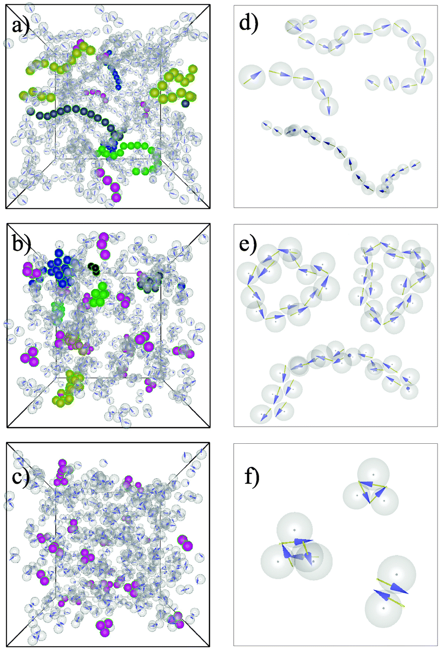 | ||
| Fig. 5 Snapshots for δ = 0 (a), δ = 0.21 (b) and δ = 0.33 (c) with revealing structures of the group (A) (a), the groups (B), (C) and (D) (b) and only (D) (c). In each snapshot, some randomly chosen clusters are coloured for a better visibility. Particles of the same color besides magenta belong to the same cluster. Magenta colored clusters represent small single clusters (D). (d–f) Magnification of randomly chosen clusters of the snap shots in the left column. | ||
Qualitatively, the structures appearing for the considered values of δ can be divided into four groups. These are chains (A), staggered chains (B), rings built by staggered chains (C) and small clusters (D) of the types presented in Fig. 10(d), 2(c) and 4(c). Structures of type (A) can consist of a few (e.g. 2–5) as well as of many (e.g. more than 10) particles, i.e., the chains can be short or long. Structures of types (B) and (C) always consist of more than 10 particles [Fig. 5(d) and (e)]. In accordance with the ground state configurations (see Fig. 2 and 4), the structures found in the finite temperature systems for different shifts pass from chainlike geometries to circular close-packed clusters upon the increase of δ. Accordingly, structures of the first group are formed for zero and small shifts in the range δ = 0.01–δ ≈ 0.1 [Fig. 5(a) and (d)]. In this shift region, the overall chainlike structure with a head-to-tail orientation as formed by nonshifted dipoles is maintained. Yet, the shift causes more and more curved structures compared to the nonshifted particles. As is generally known for dipolar systems, the chain length, i.e. the number of particles within a chain, has a polydisperse distribution.37 This holds also for the shifted system (see also the discussion of the cluster analysis in Section 5.2.2).
For intermediate shifts, e.g. δ = 0.24, Fig. 5(b) and (e), the particles within the chains become staggered and we observe the coexistence of structures of the types (B), (C) and (D). Structures of group (D) are consistent with ground state configurations of this and higher shifts. Although groups (B) and (C) are not observed for zero temperature, they can be understood as a modification of chains, as they appear for small δ, and of rings which occur at zero temperature.
If δ takes values near 0.33, all large aggregates (B) and (C) vanish and only small clusters (D) remain, as shown in Fig. 5(c) and (f).
The same structural behaviour at the different shift regions is observed for the other state points considered. Thus we conclude that the described self-assembly of the particles at different shifts is a quite general behaviour which results from the increasing dipolar coupling strength for increasing shifts. The latter causes more and more close-packed structures as we already confirmed in the case of hard spheres.
for several shifts.
The plots in Fig. 6 show g(r) for δ = 0 and δ = 0.33 for T* = 1.0 and T* = 1.35. The g(r) at zero shift is dominated by first and second neighbour correlations. This is a typical feature of strongly coupled dipolar systems38,39 and reflects the formation of chain-like structures. When we successively increase the shift, the second peak exists up to a value of δ ≈ 0.25. Beyond this value, only nearest neighbour correlations at r/σ = 1 are present in the system signifying the presence of only small and close-packed clusters (D), as seen in the snap shots of Fig. 5(c).
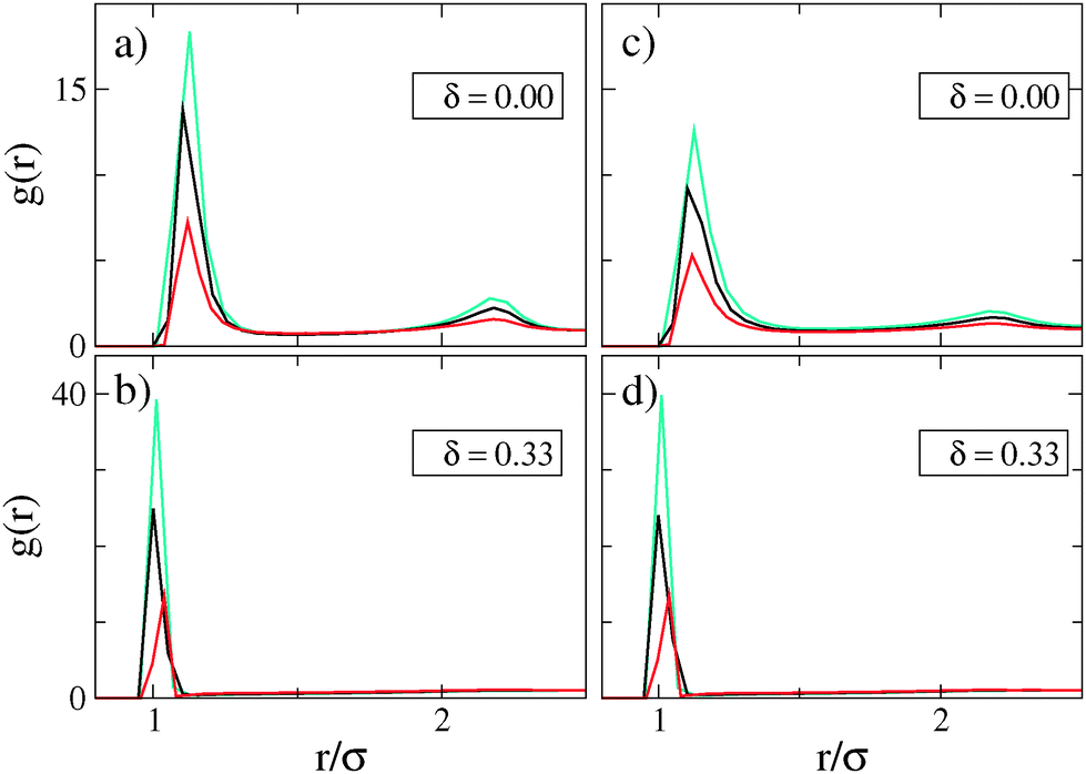 | ||
| Fig. 6 Radial distribution functions g(r) for densities ρ* = 0.07 (turquoise), ρ* = 0.1 (black) and ρ* = 0.2 (red) at two temperatures T* = 1.0 in (a) and (b), and T* = 1.35 in (c) and (d). | ||
Noticeably, the results for the higher temperature T* = 1.35 completely coincide with those of T* = 1.0 in the high shift region [Fig. 6(b) and (d)]. This is because for sufficiently high shifts, the increase of the dipolar coupling strength is already enhanced, and thus, the increase of temperature does not affect the self-assembly.
 are regarded as being clustered. Here,
  denotes the dipolar energy [see eqn (1)] between all pairs i, i′ within the critical distance rc.
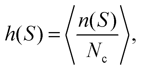
The detected clusters were collected in a histogram in which the number of clusters with size S, n(S), is counted and normalized by the total number of clusters,  , such that
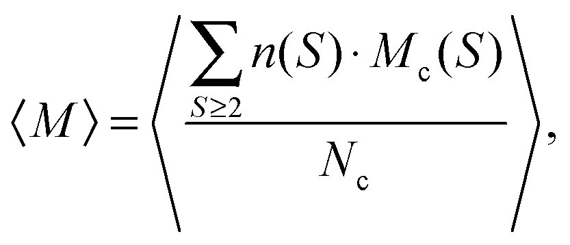
Based on the function n(S), the mean cluster magnetization is calculated by
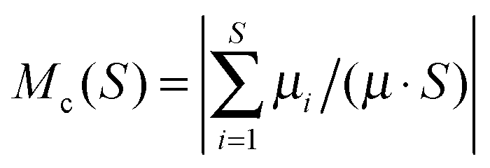 gives the normalized magnetization of a cluster with size S. The quantity Mc(S) is a measure of the parallel alignment of the dipole vectors within the individual clusters. Specifically, values of Mc(S) near to one reflect a high degree of head to tail orientation, while vanishing values of this quantity indicate an antiparallel or a triangular orientation. Therefore, mean cluser magnetization gives insights into the organization of the dipoles within the formed structures and thus allows us to evaluate if a given assembly is chainlike [types (A) and (B)] or closed [types (C) and (D)]. Note that the total magnetization, which is usually calculated by summing over all particles, has vanishing values as the system is globally isotropic at the state points considered here.
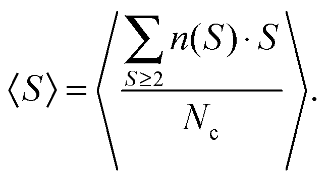
Finally, the mean cluster size is obtained from
(a) Normalised cluster size distribution. The results for h(S) for different characteristic shifts, namely for δ = 0.1 (small shift), δ = 0.16 (intermediate shift) and δ = 0.27 (high shift), are presented in Fig. 7. Fig. 7(a) and (d) show that mostly large aggregates, that can contain up to 25–30 particles, are formed. On the other hand, Fig. 7(c) and (f) indicate the formation of only small assemblies with 3–4 particles.
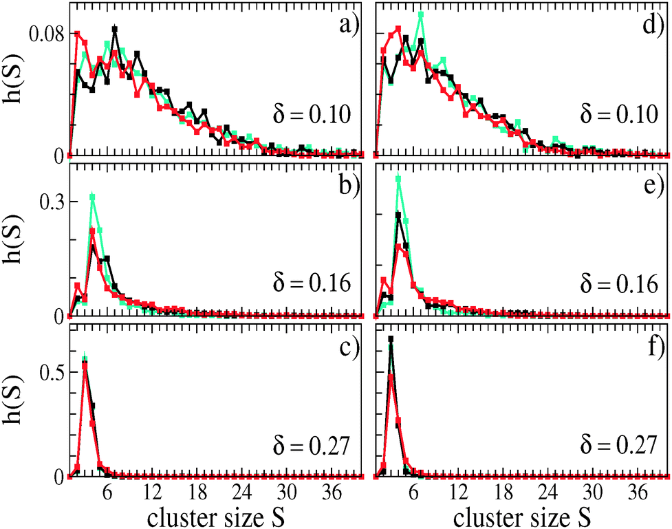 | ||
| Fig. 7 Normalized cluster size distribution for the same densities and colors as in Fig. 6: (a–c) T* = 1.0; (d–f) T* = 1.35. | ||
However, in Fig. 7(b) and (e), although there is a preferential emergence of small assemblies, large aggregates of up to 20 particles are present in a non-negligible number and secondary peaks at, e.g. S = 15 (for T* = 1.0) and S = 13 (for T* = 1.35) are visible. Evidently, for this and comparable shifts, small and large assemblies can coexist.
One also finds that for higher temperature, large aggregates are less often formed than for the smaller temperature. This is indicated by the fact that the peaks in Fig. 7(e) and (f) are enhanced compared to those in Fig. 7(b) and (c).
(c) Mean cluster magnetization. In order to evaluate the types of the occurring structures for a given shift, we determine 〈M〉 as a function of the shift and plot the results in Fig. 8(b) and (d).
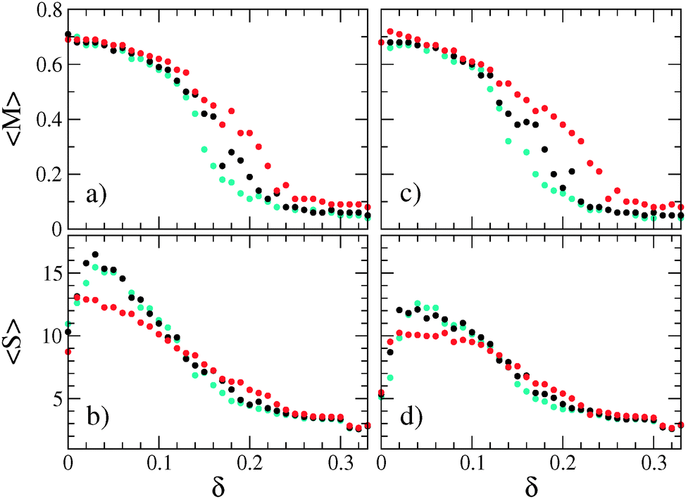 | ||
| Fig. 8 Mean cluster size 〈S〉 and mean cluster magnetization 〈M〉 as a function of the shift at two temperatures T* = 1.0 ((a), (b)) and T* = 1.35 ((c), (d)). Colors are the same as in Fig. 6. | ||
For zero and initial shifts, 〈M〉 takes the value ≈0.7, reflecting predominantly the parallel orientation of the dipoles within their aggregates. From this and from the cluster size distribution [Fig. 7(a) and (d)] we conclude that for small shifts (up to δ ≈ 0.1), mainly short and long polar chains of type (A) or (B) are formed.
If the shift is further increased, 〈M〉 decreases, indicating that polar chains occur less often. Instead, the aggregates become more and more closed structures of the types (C) or (D) with increasing shifts. Hence, the decrease of 〈M〉 implies the coexistence of types (B), (C) and (D) [see Fig. 5(b) and (e)]. At the high shift end, 〈M〉 drops down to vanishing values indicating only pairwise antiparallel or triangular arrangements of the dipoles within the clusters, which is also consisent with the results shown in Fig. 7(c) and (f). The fact that the mean cluster magnetization has vanishing values at large δ also suggests that the clusters poorly interact.
Note that for all values of δ, the corresponding aggregates are isotropically oriented such that the total magnetization is zero for all shifts (not shown here).
(b) Mean cluster size. Finally, we examine the influence of the shift on the mean cluster size and plot 〈S〉 as a function of the shift in Fig. 8(a) and (c).
Starting at δ = 0, the mean cluster size grows to its maximum with about 17 particles for T* = 1.0 and about 13 particles for T* = 1.35. The maximum is reached at δ ≈ 0.05, respectively. This increase can be understood by the effective increase of the dipolar coupling strength λ (see preceding discussion) such that initial shifts result in the formation of longer chains of type (A). If δ exceeds this value, 〈S〉 starts to gradually decrease because with increasing shift, smaller aggregates are formed more frequently (see Fig. 7). Finally, 〈S〉 attains the value of about 3 particles in the high shift end, which is a highly representative value for both temperatures considered [Fig. 7(c) and (f)]. Significant differences between the results of the two temperatures can be seen only for shifts smaller than δ ≈ 0.1 where mainly chainlike aggregates are formed. Here, the increase of temperature, which involves the decrease of the coupling strength from λ = 9 to λ ≈ 6.67, causes the formation of chains with less particles. Moreover, for these values of δ, shifting the dipoles does not impose fundamentally different self-assembly patterns compared to nonshifted dipoles. Therefore, small shifts can be regarded as perturbation of the nonshifted system.
On the other hand, high shifts impose significantly different structures: the particles exclusively form structures of type (D) that correspond to ground state configurations of two, three and four hard spheres [see Fig. 10(d), 2(c) and 4(c)]. This is possible due to the large values of λ = 72 for T* = 1 or λ ≈ 53.33 for T* = 1.35.
Finally, for intermediate shifts, where large aggregates as well as small clusters are formed, the decrease of 〈S〉 (and at the same time of 〈M〉) can be interpreted as a transition region in which large aggregates gradually dissolve into small clusters until no large structures appear at all. Within this region, the competition between energy minimization and entropy maximization results in the coexistence of both, small and large aggregates. With increasing shift (i.e., effectively increasing λ(δ)), the particles accomplish to form structures equivalent to ground state configurations.
To summarize, in the bulk systems at the finite temperatures and densities considered here, we can qualitatively distinguish between three shift regions (small, intermediate and high) each of which is characterized by its own structural characteristics. By contrast, in the ground states of two particles, we determined only a small (with head-to-tail dipolar order) and a high (with antiparallel dipolar orientation) shift region. The intermediate shift region, observed for the bulk systems, is not detected for zero temperature. This is consistent with the fact that the corresponding structures of types (B) and (C) are not observed in the ground state calculations.
6 Conclusions and outlook
In this paper, we investigated a model of spherical particles with laterally shifted dipole moments which is inspired by real micrometer sized particles that carry a magnetic component on or right beneath their surfaces (e.g.ref. 2, 8 and 9). Aiming at understanding the principal impact of the shift of the dipole moment on the self-assembly of 3D systems, we determined the ground state structures of two, three and four dipolar hard spheres. The results for two and in some extent for three particles coincide with those found in ref. 32 for a q2D system. For the three-particle case, we propose a curved chain instead of a ‘zipper’32 for very small shifts and a rectangular dipolar orientation for very high shifts. However, in all these cases, the formed structures are planar as two and three particles always lay in a plane. Most striking differences between q2D and 3D results are found for the four-particle system, for which the dimensionality of the system is crucial in view of the resulting ground state structure. In particlular, in q2D, the particles form an ideal ring32 for all shifts while in 3D, we find a cross-over from planar to out of plane structures with increasing shifts. For very high shifts, we find the tetragonal organization of the particles.Shifting the dipole does not only fundamentally affect the ground state configurations but also the self-assembly patterns in finite temperature systems. For these, we could determine three regions of shift. In each region, the self-assembly of the particles is fundamentally different. The system passes from a state which is similar to that of nonshifted dipoles to a clustered structural state. By test simulations and by comparisson with experiments,36 we estimated that shift between δ ≈ 0.25 and δ ≈ 0.3 reproduces the qualitative behaviour of Janus particles.36 Moreover, the comparison also showed that shifts larger than our choice of the limiting value δ = 0.33 is not experimentally relevant.
Further, it is an interesting observation that the asymmetry of the particles, caused by the off-centred location of the dipole moment, is overcome for small shifts insofar as the behaviour of the small shift region can be recognized as a perturbation of the nonshifted system. On the other hand, if the shift is too high, the system compensates the off-centred location of the dipole by building symmetric aggregates.
So far, we focused on the self-assembled structures at low densities. One topic of further investigations should be the interaction between the aggregates in the different shift regions. In the present study, the cluster magnetization showed a vanishing value in the high shift region which hints to a negligible interaction between the clusters. For smaller shifts, we expect similar behaviour to that for the centred system. Moreover, it would be clearly desirable to have a full phase diagram as it is known for centred dipolar soft spheres.40 A particularly interesting aspect is the impact of the shift on long-range orientational ordering. Such an investigation is clearly beyond the scope of the present paper, but will be considered in future.
In view of the severe effects of the shift on the equilibrium properties, one expects new types of pattern formation if the system is out of equilibrium. An interesting case are systems of shifted dipoles exposed to several types of external magnetic fields.41 The case of a constant field was examined in ref. 32 demonstrating that shifted dipoles form staggered chains for appropriate values for the field strength and the shift. Even more exciting phenomena are expected if the field is time-dependent, e.g. precessing or rotating. In particular, it is interesting to explore whether the model of laterally shifted dipoles is capable of describing phenomena such as the formation of a tubular8 or a crystalline structure42 accompanied by a synchronization effect. Computer simulations in these directions are on the way.
Appendix: ground state energy and configuration of two particles
In this appendix, we summarize the ground-state behaviour of two particles. Specifically, we consider the ground state energy as a function of the shift and show the appropriate ground state configurations for representative shifts.To this end, we first derive an analytical expression for the pair energies as a function of the relative shift δ = |d|/(2|R|), where |R| = σ/2 is the particle radius. A similar derivation (leading to the same result) was very recently presented in ref. 32. Here, we include the derivation as a background for investigations of N > 2 particles (see Section 4). The basis of the derivation is the coordinate system shown in Fig. 9. Note that this is a two-dimensional system (x–z-plane) where the orientations of the dipoles along the y-axis, i.e. out-of-plane orientations, are neglected. This assumption is confirmed by simulation studies of q2D dipolar systems showing that out-of-plane fluctuations vanish for decreasing temperatures.43 In Fig. 9, the angles α and β describe the orientations of the shift vectors di and dj with respect to the z-axis. As the shift vector and the dipole vector have a fixed orthogonal orientation to each other, the orientations of μi and μj with respect to the z-axis follow as α + π/2 and β + π/2. With these definitions of the angles, the results for our lateral shift can be directly compared to those for the radial shift given in ref. 27. Clearly, the distance |rij′| varies with α, β and δ. Finally, we obtain
 | (12) |
 | ||
| Fig. 9 Sketch of two dipolar hard spheres i and j and the orientations of their shift and dipole vectors in the x–z-plane. | ||
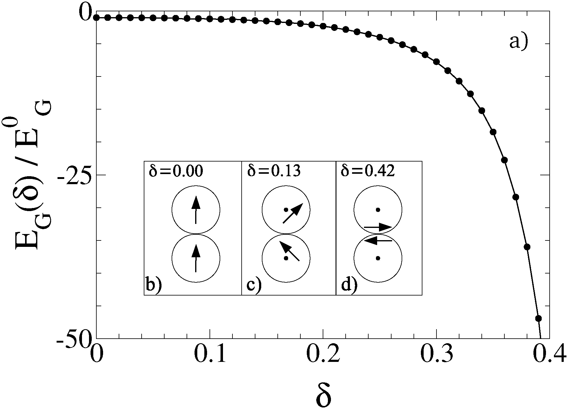 | ||
| Fig. 10 (a) Ground state pair energy EG normalized by the corresponding ground state energy E0G = −2μ2/σ3 of centred dipoles. The results are obtained by simulated annealing (circles) and by minimization of eqn (12) (solid line). (b)–(d) Ground state configurations of two dipoles. | ||
When the results shown in Fig. 10(a) are compared to the corresponding results of radially shifted dipoles of ref. 26, a qualitative agreement of the function EG(δ) can be seen. Yet, in the case of lateral shifts, the reduction of energy sets in earlier, i.e. for smaller shifts δ than those of radial shifts for which the energy starts to decrease only at δ ≈ 0.25. This can be understood by inspecting the ground state configurations corresponding to a given shift, which are shown in the inset of Fig. 10. These are determined by those values for the angles α and β that minimize eqn (12). Shifting the dipoles out of the centres, the parallel orientation of the dipoles for zero shift is gradually abandoned in favour of reducing the dipolar distance. In other words, the upper particle in Fig. 10(b) rotates clockwise while the lower one rotates counterclockwise upon increasing the shift. At the value δ ≈ 0.13, the dipoles attain a perpendicular orientation [Fig. 10(c)]. Finally, at δ = 0.2, the dipoles arrange in an antiparallel configuration of μ1 and μ2 where each of the dipoles has a perpendicular orientation relative to the connecting line between the particle centres. For all higher shifts, the antiparallel orientation is kept and only the dipolar distance is further reduced [Fig. 10(d)].
Compared to radially shifted dipoles,26 the main difference in the ground state structures is that radially shifted dipoles keep their parallel head-to-tail orientation for small shifts. Unlike laterally shifted dipoles, the antiparallel orientation is never energetically favourable. This demonstrates that not only the location but also the orientation of the dipole vector within the particle play a crucial role in the ground states of the particles.44
Acknowledgements
We gratefully acknowledge financial support from the DFG within the research training group RTG 1558 Nonequilibrium Collective Dynamics in Condensed Matter and Biological Systems, project B1. We also thank Rudolf Weeber and Christian Holm for discussions related to the derivation of the equations of motion of the laterally shifted dipoles.References
- S. H. Lee and C. M. Liddell, Small, 2009, 5, 1957–1962 CrossRef CAS PubMed.
- D. Zerrouki, J. Baudry, D. Pine, P. Chaikin and J. Bibette, Nature, 2008, 455, 380–382 CrossRef CAS PubMed.
- Y. Wang, Y. Wang, D. R. Breed, V. N. Manoharan, L. Feng, A. D. Hollingsworth, M. Weck and D. J. Pine, Nature, 2012, 491, U51–U61 CrossRef PubMed.
- S. C. Glotzer and M. J. Solomon, Nat. Mater., 2007, 6, 557–562 CrossRef PubMed.
- Y. Wang, X. Su, P. Ding, S. Lu and H. Yu, Langmuir, 2013, 29, 11575–11581 CrossRef CAS PubMed.
- B. G. P. van Ravensteijn and W. K. Kegel, Langmuir, 2014, 30, 10590–10599 CrossRef CAS PubMed.
- Q. Chen, E. Diesel, J. K. Whitmer, S. C. Bae, E. Luijten and S. Granick, J. Am. Chem. Soc., 2011, 133, 7725–7727 CrossRef CAS PubMed.
- J. Yan, M. Bloom, S. C. Bae, E. Luijten and S. Granick, Nature, 2012, 491, 578–581 CrossRef CAS PubMed.
- S. Sacanna, L. Rossi and D. J. Pine, J. Am. Chem. Soc., 2012, 134, 6112–6115 CrossRef CAS PubMed.
- D. Schamel, M. Pfeifer, J. G. Gibbs, B. Miksch, A. G. Mark and P. Fischer, J. Am. Chem. Soc., 2013, 135, 12353–12359 CrossRef CAS PubMed.
- V. S. R. Jampani, M. Skarabot, S. Copar, S. Zumer and I. Musevic, Phys. Rev. Lett., 2013, 110, 177801 CrossRef CAS PubMed.
- F. Ma, S. Wang, D. T. Wu and N. Wu, PNAS, 2015, 112, 6307–6312 CrossRef CAS PubMed.
- M. P. N. Juniper, A. V. Straube, R. Besseling, D. G. A. L. Aarts and R. P. A. Dullens, Nat. Commun., 2015, 6, 7187 CrossRef PubMed.
- J. Kotar, L. Debono, N. Bruot, S. Box, D. Phillips, S. Simpson, S. Hanna and P. Cicuta, Phys. Rev. Lett., 2013, 111, 228103 CrossRef PubMed.
- S. Jaeger and S. H. L. Klapp, Soft Matter, 2011, 7, 6606–6616 RSC.
- D. Pini, F. Lo Verso, M. Tau, A. Parola and L. Reatto, Phys. Rev. Lett., 2008, 100, 055703 CrossRef CAS PubMed.
- R. L. C. Vink, J. Horbach and K. Binder, Phys. Rev. E: Stat., Nonlinear, Soft Matter Phys., 2005, 71, 011401 CrossRef CAS PubMed.
- X. Mao, Q. Chen and S. Granick, Nat. Mater., 2013, 12, 217–222 CrossRef CAS PubMed.
- G. van Anders, D. Klotsa, N. K. Ahmed, M. Engel and S. C. Glotzer, PNAS, 2014, 111, E4812–E4821 CrossRef CAS PubMed.
- S. J. Ebbens and J. R. Howse, Soft Matter, 2010, 6, 726–738 RSC.
- F. Kogler and S. H. L. Klapp, EPL, 2015, 110, 10004 CrossRef.
- A.-P. Hynninen and M. Dijkstra, Phys. Rev. E: Stat., Nonlinear, Soft Matter Phys., 2005, 72, 051402 CrossRef PubMed.
- L. Rovigatti, J. Russo and F. Sciortino, Phys. Rev. Lett., 2011, 107, 237801 CrossRef PubMed.
- L. Rovigatti, J. Russo and F. Sciortino, Soft Matter, 2012, 8, 6310–6319 RSC.
- S. S. Kantorovich, A. O. Ivanov, L. Rovigatti, J. M. Tavares and F. Sciortino, Phys. Chem. Chem. Phys., 2015, 17, 16601–16608 RSC.
- S. Kantorovich, R. Weeber, J. J. Cerda and C. Holm, J. Magn. Magn. Mater., 2011, 323, 1269–1272 CrossRef CAS.
- S. Kantorovich, R. Weeber, J. J. Cerda and C. Holm, Soft Matter, 2011, 7, 5217–5227 RSC.
- M. Klinkigt, R. Weeber, S. Kantorovich and C. Holm, Soft Matter, 2013, 9, 3535–3546 RSC.
- L. Baraban, D. Makarov, M. Albrecht, N. Rivier, P. Leiderer and A. Erbe, Phys. Rev. E: Stat., Nonlinear, Soft Matter Phys., 2008, 77, 031407 CrossRef PubMed.
- B. Ren, A. Ruditskiy, J. H. K. Song and I. Kretzschmar, Langmuir, 2012, 28, 1149–1156 CrossRef CAS PubMed.
- A. I. Abrikosov, S. Sacanna, A. P. Philipse and P. Linse, Soft Matter, 2013, 9, 8904–8913 RSC.
- E. V. Novak, E. S. Pyanzina and S. S. Kantorovich, J. Phys.: Condens. Matter, 2015, 27, 234102 CrossRef PubMed.
- S. H. L. Klapp and M. Schoen, Rev. Comput. Chem., John Wiley & Sons, Inc., 2007, vol. 24 Search PubMed.
- M. P. Allen and D. J. Tildesley, Computer Simulation of Liquids, Oxford Science Publications, 1986 Search PubMed.
- D. Fincham, Mol. Simul., 1992, 8, 165–178 CrossRef.
- J. Yan, S. C. Bae and S. Granick, Adv. Mater., 2015, 27, 874–879 CrossRef CAS PubMed.
- P. I. C. Teixeira, J. M. Tavares and M. M. T. da Gama, J. Phys.: Condens. Matter, 2000, 12, R411 CrossRef CAS.
- D. Wei and G. N. Patey, Phys. Rev. Lett., 1992, 68, 2043–2045 CrossRef CAS PubMed.
- J. A. Moreno-Razo, E. Diaz-Herrera and S. H. L. Klapp, Mol. Phys., 2006, 104, 2841–2854 CrossRef CAS.
- D. Wei and G. N. Patey, Phys. Rev. A: At., Mol., Opt. Phys., 1992, 46, 7783–7792 CrossRef.
- S. K. Smoukov, S. Gangwal, M. Marquez and O. D. Velev, Soft Matter, 2009, 5, 1285–1292 RSC.
- J. Yan, S. C. Bae and S. Granick, Soft Matter, 2015, 11, 147–153 RSC.
- T. A. Prokopieva, V. A. Danilov, S. S. Kantorovich and C. Holm, Phys. Rev. E: Stat., Nonlinear, Soft Matter Phys., 2009, 80, 031404 CrossRef PubMed.
- J. Donaldson, E. Pyanzina, E. Novak and S. Kantorovich, J. Magn. Magn. Mater., 2015, 383, 267–271 CrossRef CAS.
| This journal is © The Royal Society of Chemistry 2016 |