A bubble-based EMMS model for pressurized fluidization and its validation with data from a jetting fluidized bed

Abstract

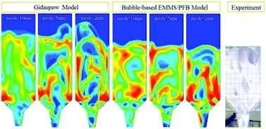
A bubble-based EMMS model for a Pressurized Fluidized Bed (PFB) was revised on the basis of an energy minimization multi-scale (EMMS) method. In the new revised model, in order to calculate the heterogeneous index accounting for the hydrodynamic disparity between heterogeneous and homogeneous fluidization, a bubble size correlation derived from experiments on a pressurized jetting fluidized bed with a conical distributor was introduced. With given operating pressure and gas superficial velocity, a heterogeneous index was calculated by integrating the bubble size correlation under elevated pressure with the EMMS model. The heterogeneous index, which decreased with the height above the distributor and also had its lowest lever when the mean voidage is in the range of (ε_mf, 1.0), was fitted into a surface and incorporated into Fluent as a user-defined function (UDF). The new bubble-based EMMS/PFB drag model was validated by predicting successfully the solid concentration distribution, the velocity of particles near the wall above the distributor, the radial profiles of particles' vertical motion and the average bubble size.

---

1. Introduction

Fluidized beds have been used in a wide range of process industries, such as chemical, petrochemical, food and pharmaceutical industries because of their enhanced gas–solid interactions.¹ It has been known that in many industrial applications, especially chemical engineering, fluidized beds are often operated in elevated pressure. Through increasing the gas density, the elevated operating pressure affects the gas–solid flow patterns and the interactions between gas and particles so as to result in obvious differences in gas–solid contacting efficiency.² Pressurized Fluidized Beds (PFB) offer several distinct advantages: high heat transfer,^3,4 strengthened gas–solid contact and mixing,⁵ high chemical reaction rate,⁶ small equipment size,⁷ and so on. The complex gas–solid hydrodynamic behavior in elevated pressure is of great importance from theoretical and practical points of view for operation, scale-up and optimization of PFB.

With the development of high performance computers and numerical algorithms, computational fluid dynamics (CFD) has become an effective way to study the gas–solid flow behaviors in fluidized bed. The two-fluid model (TFM), which assumes that the gas and solid flows were continuous, statistically averaged and fully interpenetrated into each other within each control volume,⁸ has been widely employed in various gas–solid flow researches. The physical assumption implies that homogeneous suspensions exist below the grid size and accordingly the meso-scale structures such as bubbles and clusters using TFM is much larger than the computational grid.⁹ But the fact is that the meso-scale structures described can be smaller than a coarse grid in many simulations. As a result, the accuracy of TFM with the homogeneous assumption and the scalability of simulations has been called into question.¹⁰

To take account for the influence of the heterogeneity structure of the flow, many methods are adopted in combination with the TFM, such as the energy minimization multi-scale (EMMS) model¹¹ and filtered two-fluid model.^12–16 The EMMS model developed by Li et al.¹¹ resolved the heterogeneous structure of particle–fluid flows into a particle-rich dense phase in form of clusters or aggregates and a gas-rich dilute phase in form of dispersed particles. Through solving the equations about the two phases above and their inter-phase, an EMMS drag coefficient can be obtained and accordingly coupled with TFM in simulation. A great deal of researches with the employment of the EMMS model have derived reasonable results which agree with the experiments well.^17–24 The original EMMS model was based on the concept of particles cluster and mainly applied to high-velocity circulating fluidized beds. The subsequent bubble-based EMMS model¹⁰ with replacement of particles clusters by bubbles was proposed for applications in bubbling fluidizations. Though the bubbles and clusters belong to the same family of non-uniform hydrodynamic solutions,²⁵ it's easier to describe bubbles compared with the cluster. Many correlations of bubble size in the literatures^26–28 are available for bubble-based EMMS model solution, among which Moro's correlation is adopted by Hongkun²⁹ to simulate the flow in a CFB riser. However, the correlations mentioned above did not take the effect of operating pressure into consideration and little research pays attention to simulation of pressurized fluidized bed with the EMMS model. Bubble behaviors such as the size in pressurized fluidized bed determine the fluidization quality and therefore, a suitable correlation is of great importance for the accuracy of the simulation. In this paper, a bubble-based EMMS/PFB model is revised by introducing a bubble size correlation derived from experiments on a pressurized jetting fluidized bed with conical distributor. Gas–solid flow behavior of a pressurized jetting fluidized bed is simulated by coupling the new revised bubble-based EMMS/PFB model with the TFM and the results are compared to experimental data for verification.

2. Descriptions of bubble-based EMMS/PFB model

The flow in pressurized fluidized bed is usually resolved into a gas-rich dilute phase in form of bubbles or voids, coexisting a particle-rich dense phase in form of emulsions, as shown in Fig. 1. The volume fraction is δ_b for dilute phase 1 − δ_b for dense phase. The voidage is ε_ge and superficial velocity of gas and particles is U_ge and U_pe, respectively, in dense phase. For the sake of simplicity, dilute phase is assumed only consisting of gas with velocity of U_b and the diameter of bubble is d_b. For the unsteady flow, the acceleration of particles in dense phase a_e and dilute phase a_b are introduced to consider the inertia force. The dense phase is assumed as a homogeneous mixture and can be viewed as a pseudo-fluid with mean density ρ_e, viscosity μ_e (ref. 30) and superficial velocity U_e, as follows:

ρ_e = ρ_gε_ge + ρ_p(1 − ε_ge) (1)

μ_e = μ_g[1 + 2.5(1 − ε_ge) + 10.05(1 − ε_ge)² + 0.00273 exp(16.6(1 − ε_ge)) (2)

Fig. 1 System resolution for pressurized fluidized bed.

Table 1 summarizes the relevant parameters and formula of this model. For a given system with specified conditions (U_g, U_p and ε_g), the flow states can be described by the eight parameters mentioned above (δ_b, ε_ge, U_b, U_ge, U_pe, d_b, a_e, a_b). A whole set of balance equations can be built through the multi-scale analysis method to solve the parameters. It is assumed that the structure-dependent drag coefficient is isotropic when EMMS drag is coupled with TFM model, but only the scalars of vertical components are used in the bubble-based EMMS model analysis.

Table 1 The parameters and formula in the model

	Emulsion phase	Inter-phase
Characteristic diameter	dp	db
Voidage	εge	δb
Superficial slip velocity		Uslip,i = (1 − δb)(Ub − Ue)
Characteristic Reynolds number
Standard drag coefficient^28
Effective drag coefficient^31	Cde = Cde0εge^−4.7	Cdi = Cdi0(1 − δb)^−0.5
Number density
Drag force on each particle or bubbles
Drag force in unit volume	Fde = meFe	Fdi = miFi

---

2.1 The bubble size correlation for PFB

Bubble size is one of the most important parameters of gas–solid fluidized beds. Most rate phenomena in fluidized beds such as bubble rising velocity, gas rate of interchange between phases and heat transfer depends on the bubble size. Reliable correlation of bubble size is of great importance for the design and accurate modeling of fluidized bed. Many correlations has been built for prediction of bubble size in the literature,^26–28 in which excess velocity (U_g − U_mf) and vertical distance from the distributor H are involved. However, lots of experimental data show that the bubble size varies with operating pressure P. It's recognized that the bubble size decreases with increasing operating pressure P in both the bubbling and turbulent regimes except when gas velocity is very low,³² as shown in Fig. 2.

Fig. 2 Bubble size varies with pressures and velocity by P. Cai.³²

Thanks to the enhanced gas–solid interactions in the region above the jet, pressurized jetting fluidized beds are widely used in many industries such as chemical, pharmaceutical, and petrochemical. Different purposes can be accomplished by adjusting the designed velocity introduced from jets: to enhance mixing and heat transfer, supplement the reactant, control the reactions, or prevent slugging in the bed.¹ In the pressurized jetting fluidized bed, the fluidization gas enters from the conical distributor and the jetting gas from the central jet. Flowing through the bed, the jetting gas will spread to the surrounding area from the centre of the bed and at the same time get the fluidization gas mixed up in the central gas. For most process such as coal gasification, the interaction between the fluidization gas and the jetting gas will promote the mass and heat transfer and strength the gas–solid contact. Furthermore, the conical distributor has the advantages of better anti-slagging compared with the plate distributor. However, everything has two sides, it also makes the bubble behaviors in the pressurized jetting fluidized bed more complex, which means more effort is needed to get reliable flow information in the bed.

In order to achieve the bubble size correlation, a bubble dynamics experiment was performed on a pressurized jetting fluidized bed.³³ The experimental device is mainly composed of a two-dimensional jetting fluidized bed fluidized bed, a liquid nitrogen gas supply system, a pressure chamber, a mass flow meter, a probe fiber velocity measuring system and a camera system as shown in Fig. 3. A transparent Plexiglas jetting fluidized bed with 300 × 30 mm is put into the pressure chamber to study the movement of the particles. The fluidization gas supply for fluidized bed and pressurization gas supply for pressure chamber is provided by liquid nitrogen supply system. Flow control is accomplished by a parallel mass flow meter setup. The pressure chamber (Φ 1200 × 1600 mm) is capable of operating at design pressure up to 3.3 MPa. The velocity of particles is measured by PV-6 probe fiber velocimetry. Several CCD cameras are set into the chamber to record the flow information inside the bed.

Fig. 3 Scheme of the experimental set-up: (1) computer; (2) data processing system; (3) mass flow meter/controller; (4) pressure vessel; (5) optical fiber probe; (6) two dimensional jetting fluidized bed; (7) LED lamps; (8) CCD camera.

The bubble information including shape, size, position and velocity is obtained by data treatment of the bubble images captured by CCD cameras. First, the fluidization in the bed is obtained on the desired pressure provided by the pressure vessel through the liquid nitrogen supply system. Then, several CCD cameras are employed to record the bubble information as a video, which is converted into a series of single image for subsequent data analysis. The size and position coordinate of bubbles can be extracted by image analysis software through the gray scale difference between bubbles and their surroundings. At the same time, the bubble rising velocity is calculated by the position change of the same bubble in two adjacent images.

Many correlations has been built for prediction of bubble size in the literature, among which P. Cai³² developed a generalized correlation which fitted the experimental data quite well for pressurized fluidized bed combustors. However, the influences of the angled distributor and the jetting gas velocity were not taken into account in P. Cai's correlation. As the same form of P. Cai's correlation, a new revised correlation with consideration of the factors mentioned above was achieved based on the experimental data obtained, as follows:

where H is the height of a bubble from the distributor and H₀ is a constant through experimental observation and data analysis (H₀ = 0.1 when H ≤ 0.09 m and H₀ = 0.08 when H > 0.09 m), P is the operating pressure, (U_g − U_mf) is excess gas velocity, U^Θ_t, U_t are the terminal velocity of particles under ambient and elevated pressure, U_j is jetting gas velocity and the constants a = 0.0003, b = 0.25, c = 0.1, d = 3.

Theoretically, the correlation is applicable to pressurized systems with central jetting and angled distributor gas inlet, in both bubbling and turbulent fluidization for group B particles like P. Cai's correlation. Correspondingly, the correction terms may change with the size and operation parameters of pressurized systems. Fig. 4 shows the bubble diameters from experiment in this study (P = 0.7 MPa, U_f − U_mf = 0.3(0.35) m s⁻¹) and calculation through eqn (4) fitted by averaged experimental data. The computed value is slightly higher than the measured value, the reason for which may lie in the inevitable errors in the extraction and measurement of bubbles. The average errors of the fitting are ±12.6% for relative values, which is acceptable to use in the solution of the nonlinear equations in the EMMS model below.

Fig. 4 Bubble size varies with height above distributor through experiment on the pressurized jetting fluidized bed and calculation from the correlation of eqn (4).

2.2 Balance equations for both phases in the cells

Force balance for particles in the dense phase in unit volume: the drag force of the dense phase gas is equal to the effective weight of the particles inside the dense phase. Due to the inertia difference of the gas and particles in the dense phase is very large, the acceleration a_e of the particles in the dense phase can be ignored,³⁴ that is a_e = 0.

Force balance for the inter-phase: the drag force on the inter-phase counterbalance the effective gravity.

Mass balance for the gas and particles: the net mass flow rate of the gas phase through any cross-section of the bed should be equal to the sum of the gas flow rate through both the dilute and dense phases. And the net mass flow rate of the particles through any cross-section should be equal to the sum of the particle flow rate through both the dilute and dense phases.

U_g = U_ge(1 − δ_b) + U_bδ_b (7)

U_p = U_pe(1 − δ_b) (8)

The overall voidage of the system is calculated through the voidage of the dense phase and dilute phase as follows:

ε_g = ε_ge(1 − δ_b) + ε_gbδ_b (9)

2.3 Minimization of energy consumed by drag force

From the analysis above, it can be found that the number of equations (eqn (4)–(9)) is less than the amount of independent variables (δ_b, ε_ge, U_b, U_ge, U_pe, d_b, a_b), so an extra constraint is needed to close such optimization problems as pointed out in Li and Kwauk.¹¹ In the fluidized bed, the particles and the gas can not control each other and fully realize their own movement trend. They have to compromise with each other in such a way that the gas suspends particles with least energy consumption and meanwhile flows through particles with minimum resistance. In this situation, the energy consumption rate for suspending and transporting a unit mass particles tends to minimum. The stability condition for a bubbling fluidized bed is that the mass-specific energy consumption rate for suspending energy reformulated by Shi et al.¹⁰ tends to minimum energy:where f_b is the ratio of gas in the bubble phase to that in total expressed as follows:

From the analysis above, we can find that all the parameters involved (δ_b, ε_ge, U_b, U_ge, U_pe, d_b, a_b) can be solved by introducing the stability condition as an optimization function. Once the structural parameters in the model are determined, the effective drag coefficient can be calculated as:¹⁷

A heterogeneous index is defined to describe the influence of heterogeneous structure on the drag coefficient as follows:

where β_w (ref. 35) is the commonly used form of the drag coefficient without considering the influence of heterogeneous structure.

2.4 Solution scheme and heterogeneity index analysis

There are 7 parameters to be solved (δ_b, ε_ge, U_b, U_ge, U_pe, d_b, a_b) to be solved with 6 conservation equations (eqn (4)–(9)) available. Hence, the objective function eqn (10) is very necessary. A global search scheme to get the set of 7 parameters that satisfies both the conservation equations and the constraint of minimum is adopted to solve the nonlinear programming problem as follows:

(1) For the given system with the operating pressure P, the superficial gas velocity U_g and physical parameters (ρ_p, ρ_g, μ_g), assign a big value for N_st and traverse the vertical height from the distributor H within the whole height of the bed, then calculate d_b from eqn (4).

(2) Sweep ε_g within the range of (ε_mf, 1.0). Sweep ε_ge within the range of (ε_mf, ε_g).

(3) Calculate δ_b from eqn (9).

(4) Calculate U_slip,e from eqn (5), then U_ge from the definition equation of U_slip,i in Table 1.

(5) Calculate U_b from eqn (7), then calculate U_e from eqn (3), calculate U_slip,i from the definition equation of U_slip,i in Table 1.

(6) Calculate a_b from eqn (6).

(7) Calculate N_st from eqn (10), store it and the relevant set of six parameters if N_st is smaller than the previous values.

(8) Complete the sweeps of H, ε_g and ε_ge, and then output the set of six parameters corresponding to minimum N_st.

(9) Calculate each β_e-bubble and H_d, then correlate the parameters into H_d = f(H,ε_g).

The analysis presented in this work is based on the pressurized bubbling fluidized bed experiment system (P = 0.7 MPa, ρ_g = 7.87 kg m⁻³, ρ_s = 1020 kg m⁻³, d_p = 132 μm, U_g = 0.74m s⁻¹ and 2.1 m s⁻¹, U_mf = 0.19 m s⁻¹, H = 0–1 m).

Fig. 5 shows the variation of heterogeneity index H_d with mean voidage ε_g and vertical distance from distributor H. In comparison with the Shi et al.'s scheme and correlation,¹⁰ H_d shows a drop with increase of the vertical distance from distributor H as shown in Fig. 5, the reason for which possibly be that when H becomes large, the size of bubble becomes bigger and the heterogeneity effect is strengthened. The heterogeneity index gap due to the vertical distance from distributor H is not negligible and it's very necessary to consider the influences of parameter H for the drag in the simulation. Another distinguished feature of Fig. 5 is that H_d has its lowest lever when the mean voidage is in the range of (ε_mf, 1.0). The reason may be that the bed gradually transforms into a uniform fluidization state near two ends of the curve H_d. Associate H_d with mean voidage ε_g and vertical distance from distributor H, a surface map can be derived as shown in Fig. 6. To verify this bubble-based drag model, a fitting equation about the surface map (seen in Table 2) is used to couple TFM with this new drag model.

Fig. 5 Variation of heterogeneity index H_d with ε_g and H (a) U_g = 0.74 m s⁻¹ and (b) U_g = 2.1 m s⁻¹.

Fig. 6 Surface of heterogeneity index H_d with ε_g and H (a) U_g = 0.74 m s⁻¹ and (b) U_g = 2.1 m s⁻¹.

Table 2 The correlation of H_d with ε_g and H in given operation parameters

a Where ε_d denotes the voidage at the intersection of the H_d function and unity.

---

3. Simulation results and discussions

3.1 TFM with the bubble-based EMMS/PFB model

In order to limit the computational cost, the Eulerian TFM is adopted in the present work. The conservation of mass and momentum of both phases is considered in the TMF computation since the solid phase is assumed as a fluid. The solid stress in the momentum equations for solid phase is closed with the kinetic theory of granular flows (KTGF), in which the conservation of solid fluctuation energy is considered.³⁶ The governing equations including the conservation equations and constitutive correlations for solid stress and interfacial drag coefficient are summarized in Table 3. The bubble-based EMMS/PFB drag is incorporated into Fluent as a user-defined function (UDF).

Table 3 Hydrodynamic equations

Continuity equations
	(T1-1)
	(T1-2)
Momentum equations
	(T1-3)
	(T1-4)
Gas/solid phase stress
	(T1-5)
	(T1-6)
Solid phase shear viscosity
μs = μs,col + μs,kin + μs,fr	(T1-7)
	(T1-8)
	(T1-9)
	(T1-10)
Gas/solid phase bulk viscosity
λg = 0	(T1-11)
	(T1-12)
Radial distribution function
	(T1-13)
Solid pressure
ps = εsρsθs + 2ρs(1 + ess)g0εs^2θs	(T1-14)
Granular temperature
	(T1-16)
Drag coefficient of gas–solid
	(T1-17)
	(T1-18)
	(T1-19)
	(T1-20)

---

3.2 Simulation settings and boundary conditions

Numerical simulations described here to test the bubble-based EMMS/PFB drag model are based on the pressurized jetting fluidized bed experiment, for which reliable experimental data is available for comparison. The detailed parameters of simulation and experiment are summarized in Table 4.

Table 4 Summary of simulation settings in Fluent

Symbol	Description	Unit	Simulations	Experiment
P	Operating pressure	MPa	0.7	0.7
ρp	Density of particles	kg m^−3	1020	1020
ρg	Gas density	kg m^−3	Changes with pressure	Changes with pressure
dp	Diameter of particles	m	0.00132	0.00132
μg	Gas viscosity	Pa s	Changes with pressure	Changes with pressure
εs,max	Packing limit	—	0.63	—
umf	Minimum fluidization velocity	m s^−1	0.19	0.19
esw	Particle–wall coefficient restitution	—	0.99	—
ess	Particle–particle coefficient restitution	—	0.9	—
ϕ	Specularity coefficient	—	0.0001	—
h0	Initial bed height	m	0.45	0.45
Δt	Time step	s	0.0001	—

---

3.3 Turbulence model

The dispersed standard k–ε model is used in this study. k–epsilon (k–ε) turbulence model is the most common model used in CFD to simulate mean flow characteristics for turbulent flow conditions because of its good calculation accuracy. The turbulence equations are solved for the gas phase, and the turbulence parameters for the solid phase are deducted using dispersion rules:³⁷where G_k,g represents the generation of turbulence kinetic energy due to the mean velocity gradients. The model constants have their default values C_1ε = 1.44, C_2ε = 1.92, σ_k = 1.0, σ_ε = 1.3 as default and the subscript g represents a gas phase.

The size of the experimental pressurize jetting fluidized bed is 300 × 800 × 30 (mm) above the distributor, which may therefore be considered as a 2 dimensional geometry. Therefore, 2-D simulation is adopted in order to reduce computation time in this study. Fig. 7 sketches the simulated 2D pressurized fluidized bed. Quadrilateral meshes are generated with the type of pave at the scales of 2 mm, 5 mm, and 10 mm, respectively. Correspondingly, the total mesh set consists of 71 076, 11 314 and 2884 cells. Considering the accuracy of the results and the computation time cost by comparison of the above 3 mesh schemes (seen as Fig. 8), 5 mm mesh size was adopted afterwards if there is no special statement in this study.

Fig. 7 Schematic drawing of the bubbling bed in simulation.

Fig. 8 Instantaneous solid concentration in the bubbling bed.

The gas flows into the pressurized bed through the bottom inlet and the distributor respectively and leaves from the top outlet, where 0.7 MPa pressure is set by prescribing operating pressure boundary condition. Initially, the solid particles are uniformly distributed in the bed with a fixed voidage which is estimated from experimental data. The no-slip boundary was prescribed for the gas, while the partial–slip boundary developed by Johnson and Jackson³⁸ was adopted for the solids with the specularity coefficient 0.6. Other detailed simulation setting parameters are list in Table 4.

In order to obtain the detailed information of the bubbling bed, two measurement points are also set on the jetting fluidized bed, as shown in Fig. 7, while the lower measurement point's coordinate (code named LBH) is x = 135 mm, y = 90 mm and the upper measuring point's (code named HBH) coordinates is x = 135 mm, y = 150 mm, as shown in Fig. 7.

3.4 Simulation results and discussions

3.4.1 The snapshots of solid concentration distribution. Simulations lasted for 20 s in physical time and the time-average variables were obtained over the range 5–15 s. Fig. 8 demonstrates the solid distribution in the pressurized jetting fluidized bed computed with drag coefficient of Gidaspow model and the new revised bubbling-based EMMS/PFB model, respectively, under different grid resolutions (grid size = 2 mm, 5 mm and 10 mm). The bed expansion is overestimated using the Gidaspow model compared with the revised bubbling-based EMMS/PFB model. The results reveal that the bubble-based EMMS/PFB drag model can capture obvious heterogeneous bubbling even with a relatively courser grid size of 10 mm. In contrast, the Gidaspow drag model with the grid size of 10 mm gives relatively uniform distribution except bubbling near the bottom due to intensive mixing near the gas inlets.

3.4.2 The velocity of particles near the wall above the distributor. The particles near the wall above the distributor of a jetting fluidized bed usually move slowly and therefore local hot spots will form for a combustion or gasification fluidized bed because the heat from coal combustion there cannot be taken away in time. In particular, with the increase of operating pressure, coal combustion or gasification reaction rate and the heat and mass transfer between two phases are accelerated which will result in slagging easily. So, more studies are needed on the motion of particles near the wall of the jetting fluidized bed under elevated pressure.

In the simulations, the velocity both on the points LBH and HBH was monitored and the time–averaged values of velocity can be calculated. Both the drag models seem to reach their converged velocity. As shown in Fig. 9, on the point LBH, the predicted values of velocity are about 0.80 m s⁻¹ from the Gidaspow drag model and 0.61 m s⁻¹ from the new revised bubble-based EMMS/PFB drag model, respectively, while the experiment date is 0.55 m s⁻¹. And on the point HBH, the predicted values of velocity are about 1.38 m s⁻¹ from the Gidaspow drag model and 1.04 m s⁻¹ from the new revised bubble-based EMMS/PFB drag model, respectively, while the experiment date is 0.91 m s⁻¹. Obviously, the EMMS drag predicts the experimental value of velocity well.

Fig. 9 Velocity of particles on the location of LBH (a) and HBH (b).

3.4.3 The radial profiles of particles vertical motion. Fig. 10 compares the radial profiles of particles vertical motion computed by the new revised bubble-based EMMS/PFB drag model and Gidaspow model at the height of 0.09 m and 0.15 m, respectively. The particles move downwards near the wall and upwards at the center. Compared with the new revised bubble-based EMMS/PFB drag model, the Gidaspow model gives a more steep profile due to the overestimated drag coefficient.

Fig. 10 Radial time–averaged velocity profiles of particles at the height of 0.09 m (a) and 0.15 m (b).

Though the revised bubble-based EMMS/PFB drag model and Gidaspow model are both with same trend and order for the solid velocity predictions, the former has a higher accuracy. Bubbles, one of the main meso-scale performance, have a great influence on the inter-phase heat and mass transfer. The bubble-based EMMS/PFB drag model can capture more obvious bubbles, even with a relatively courser grid size of 10 mm, as seen in Fig. 8. This is very valuable in engineering scale bed simulation.

3.4.4 The average bubble size by simulation. As mentioned above, bubble size is a very important parameter of gas–solid fluidized beds because that most rate phenomena in fluidized beds such as mass and heat transfer between phases depends on the bubble size. Fig. 11 compares the average bubble size by simulation and experiment. Fairly good agreement between them can be observed.

Fig. 11 Comparison of the average bubble size by experiment and simulation.

4. Conclusion

A multi-scale model following the method of EMMS for scale resolution and energy consumption criterion is revised for pressurized fluidized bed, through combination a bubble size correlation under elevated pressure on the basis of experiment. It gives an insight on the application to simulation the flow behavior from bubbling fluidization to turbulent fluidization in pressurized fluidized bed. With given operating pressure and gas superficial velocity, a heterogeneous index was fitted into a surface with gas voidage and the height above the distributor and incorporated into Fluent as a user-defined function (UDF). Simulations of flow behavior in a laboratory scale pressurized jetting fluidized bed were performed by coupling of the new bubble-based EMMS/PFB drag model with the traditional TFM. The new model predicted successfully the solid concentration distribution, the velocity of particles near the wall above the distributor, the radial profiles of particles vertical motion and the average bubble size. It's a long-term target to explore more extensive applications for the bubble-based EMMS/PFB model and more efforts on verification of the model still should be taken in future studies.

Abbreviations

ab	Acceleration of bubble, m s^−2
ae	Acceleration of particles in emulsion, m s^−2
C1ε	Model constant in standard k–ε model, dimensionless
C2ε	Model constant in standard k–ε model, dimensionless
Cam	Coefficient of added mass force, dimensionless
Cde	Effective drag coefficient for a particle in emulsion phase, dimensionless
Cde0	Standard drag coefficient for a particle in emulsion phase, dimensionless
Cdi	Effective drag coefficient for inter-phase, dimensionless
Cdi0	Standard drag coefficient for a bubble, dimensionless
Cd0	Standard drag coefficient for a particle, dimensionless
db	Bubble diameter, m
dp	Particle diameter, m
Fam	Added mass force per unit volume, kg m^−2 s^−2
fb	Ratio of gas in the bubble phase to that in total, dimensionless
Fde	Drag force of emulsion phase in unit volume, (kg m^−2 s^−2)
Fdi	Drag force of bubble in unit volume, (kg m^−2 s^−2)
Fdb	Drag force of bubble phase in unit volume, (kg m^−2 s^−2)
Fe	Drag force on each particle in emulsion phase, (kg m^−2 s^−2)
Fi	Drag force on each bubble in inter-phase, (kg m^−2 s^−2)
G	Gravity acceleration, m s^−2
H	Vertical distance from the distributor, m
Hd	Heterogeneous index, dimensionless
me	Number density of emulsion phase, dimensionless
mi	Number density of inter-phase, dimensionless
Nst	Energy consumption for suspending and transporting particles, J s^−1 kg^−1
P	Operating pressure, MPa
Ree	Characteristic Reynolds number of emulsion phase, dimensionless
Rei	Characteristic Reynolds number of inter-phase, dimensionless
Rei	Characteristic Reynolds number, dimensionless
Ub	Superficial gas velocity in the bubble phase, m s^−1
Ue	Average superficial velocity of the emulsion phase, m s^−1
Uf	Distributor gas velocity, m s^−1
Ug	Superficial gas velocity, m s^−1
Uj	Jetting gas velocity
Ugb	Superficial gas velocity in the bubble phase, m s^−1
Uge	Superficial gas velocity in the emulsion phase, m s^−1
Up	Superficial particle velocity, m s^−1
Upe	Superficial particle velocity in the emulsion phase, m s^−1
Umf	Superficial gas velocity at minimum fluidization, m s^−1
Uslip	Superficial slip velocity, m s^−1
Uslip,e	Superficial slip velocity of emulsion phase, m s^−1
Uslip,i	Superficial slip velocity of inter-phase, m s^−1
U^Θt	Terminal velocity of particles under ambient pressure, m s^−1
Ut	Terminal velocity of particles under elevated pressure, m s^−1
ag	Volume fraction of gas phase in k–ε model, dimensionless
βe-bubble	Effective drag coefficient with structure in a control volume, kg m^−3 s^−1
βw	Effective drag coefficient without structure in a control volume, kg m^−3 s^−1
δb	Volume fraction of bubble phase
εg	Voidage
εmf	Incipient voidage
σk	Model constant in standard k–ε model, dimensionless
σs	Model constant in standard k–ε model, dimensionless

Acknowledgements

This work was financially supported by the National Natural Science Foundation of China (No. 21606250, 21506242), the Natural Science Fund of Shanxi Province (2014021014-7) and the Strategic Priority Research Program of the Chinese Academy of Sciences, Multi-stage conversion fluidized bed coal gasification technology and pilot plant research (XDA0705 0100).

Notes and references

1. T. Wang, T. Tang, Y. He and H. Yi, Chem. Eng. J., 2016, 283, 127–140.
2. J. A. M. K. Jie Li, Powder Technol., 2002, 127, 173–184.
3. Z. Li, M. v. S Annaland, J. A. M. Kuipers and N. G. Deen, Chem. Eng. Sci., 2016 DOI:10.1016/j.ces.2016.04.046.
4. P. B. Nyoman and S. Winaya, Int. J. Heat Mass Transfer, 2001, 44, 2965–2971.
5. P. A. Olowson and A. E. Almstedt, Chem. Eng. Sci., 1990, 45, 1733–1741.
6. J. Cao, Z. Cheng, Y. Fang, H. Jing, J. Huang and Y. Wang, Powder Technol., 2008, 183, 127–132.
7. S. Valin, S. Ravel, J. Guillaudeau and S. Thiery, Fuel Process. Technol., 2010, 91, 1222–1228.
8. D. Gidaspow, Multiphase Flow and Fluidization, Academic Press, Boston, 1994.
9. K. Hong, Z. Shi, A. Ullah and W. Wang, Powder Technol., 2014, 266, 424–432.
10. Z. Shi, W. Wang and J. Li, Chem. Eng. Sci., 2011, 66, 5541–5555.
11. J. Li and M. Kwauk, Particle–Fluid Two Phase Flow: Energy-minimization Multi-scale Method, Metallurgical Industry Press, Beijing, 1994.
12. L. Yin, S. Wang, H. Lu, S. Wang, P. Xu, L. Wei and Y. He, Chem. Eng. Sci., 2010, 65, 2664–2679.
13. Y. Igci, A. T. Andrews, S. Sundaresan, S. Pannala and T. O'Brien, AIChE J., 2008, 54, 1431–1448.
14. W. Holloway and S. Sundaresan, Chem. Eng. Sci., 2012, 82, 132–143.
15. S. S. Ozarkar, X. Yan, S. Wang, C. C. Milioli, F. E. Milioli and S. Sundaresan, Powder Technol., 2015, 284, 159–169.
16. W. Shuai, X. Pengfei, L. Huilin, Y. Yunchao, Y. Lijie and W. Jiaxing, Chem. Eng. Sci., 2011, 66, 593–603.
17. W. Wang and J. Li, Chem. Eng. Sci., 2007, 62, 208–231.
18. N. Yang, W. Wang, W. Ge and J. Li, China Particuol., 2003, 1, 38–41.
19. A. Nikolopoulos, K. Atsonios, N. Nikolopoulos, P. Grammelis and E. Kakaras, Chem. Eng. Sci., 2010, 65, 4089–4099.
20. B. Lu, N. Zhang, W. Wang and J. Li, Particuology, 2012, 10, 663–671.
21. J. Wang, Q. Zhou, K. Hong, W. Wang and J. Li, Chem. Eng. Sci., 2012, 75, 349–358.
22. M. Zeneli, A. Nikolopoulos, N. Nikolopoulos, P. Grammelis and E. Kakaras, Chem. Eng. Sci., 2015, 138, 482–498.
23. M. Zhao, N. Zhang, X. Liu and W. Du, Powder Technol., 2015, 284, 443–451.
24. Q. Zhou, J. Wang and J. Li, Chem. Eng. Sci., 2014, 107, 206–217.
25. B. J. Glasser, S. Sundaresan and I. G. Kevrekidis, Phys. Rev. Lett., 1998, 81, 1849–1852.
26. A. N. Masayuki Horio, AIChE J., 1987, 33, 1865–1872.
27. S. Mori and C. Y. Wen, AIChE J., 1975, 21, 109–115.
28. R. C. Darton and D. Harrison, Trans. Inst. Chem. Eng., 1974, 52, 301–306.
29. K. Hong, Z. Shi, A. Ullah and W. Wang, Powder Technol., 2014, 266, 424–432.
30. D. G. Thomas, J. Colloid Sci., 1965, 20, 267–277.
31. M. Ishii and N. Zuber, AIChE J., 1979, 25, 843–855.
32. M. S. P. Cai and G. De Michele, Powder Technol., 1994, 80, 99–109.
33. L. Junguo, Hydrodynamic Characteristics in Jetting Fluidized Bed under Pressure, University of Chinese Academy of Sciences, 2013.
34. Z. Shi, A Bubble-based EMMS Model for Gas-solid Fluidized Beds and Its Application in CFD Simulation of a Coal Gasifier, University of Chinese Academy of Sciences, 2011.
35. C. Y. Wen and Y. H. Yu, Chem. Eng. Prog., Symp. Ser., 1966, 62, 100–111.
36. D. Gidaspow, Multiphase flow and fluidization: Continuum and kinetic theory descriptions, Academic Press, San Diego, 1994.
37. Z. Xia, Y. Fan, T. Wang, X. Guo and C. Chen, Chem. Eng. Sci., 2015, 131, 12–21.
38. P. C. Johnson and R. Jackson, J. Fluid Mech., 1987, 176, 67–93.

---