Sustainable development of coconut shell activated carbon (CSAC) & a magnetic coconut shell activated carbon (MCSAC) for phenol (2-nitrophenol) removal

Abstract

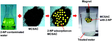
Slow pyrolysis coconut shell (CSAC) and magnetic coconut shell (MCSAC) activated carbons were prepared, characterized and used for aqueous 2-nitrophenol (2-NP) removal. Magnetization was carried out using a co-precipitation method. The chemical composition, surface properties and morphology were examined using proximate and ultimate analyses. The carbons were microporous with a BET surface area of 607 m² g⁻¹ (CSAC) and 407 m² g⁻¹ (MCSAC). Both batch and column studies were conducted. The carbons efficiently remediated 2-nitrophenol (2-NP) contaminated water at pH 4.0. Sorption equilibrium studies were conducted at 25, 35, and 45 °C. Experimental data were fitted to Langmuir, Freundlich, Sips, Temkin, Redlich–Peterson, Radke and Prausnitz, Toth, and Koble–Corrigan equations. Sips and Koble–Corrigan equations best fitted the 2-NP adsorption data. A pseudo-second-order model best described the kinetics data. Columbic interactions, hydrogen bond formations, π–π donor–acceptor interactions, and dipole–dipole interactions were the possible mechanisms for 2-NP removal. MCSAC was easily recovered from an aqueous system using an external magnet and successfully regenerated using methanol. Fixed-bed studies were conducted at room temperature with an initial 2-NP concentration of ∼13 mg L⁻¹, 2.0 g CSAC, pH 4.0 and a flow rate of 4 mL min⁻¹. A column capacity of 102.8 mg g⁻¹ was obtained. 2-NP desorption was also carried out under the same flow rate, and bed height using ten successive aliquots each containing 20 mL of methanol. The first aliquot of 20 mL of methanol desorbed 48% of the total 2-NP recovered and the rest in the further nine increments. These studies clearly demonstrated that developed carbons can serve as potential sorbents for phenol removal to substitute expensive commercial activated carbons.

---

1. Introduction

Phenols are among the most important and serious organic pollutants.^1,2 They are listed as one of the priority pollutants.³ The United States Food and Drug Administration (USFDA) and World Health organization (WHO) recommend a permissible limit of 0.001 mg L⁻¹ phenols in drinking water.^4,5 The Bureau of Indian Standards (BIS) has prescribed 0.002 mg L⁻¹ as a permissible limit for phenols in drinking water.⁶ The major sources of phenolic input to the water bodies include effluents from coke ovens in steel plants, petroleum refineries, petrochemical, phenolic resin, and fertilizer, pharmaceutical, chemical, dye industries, coal processing, plastics, wood products, pesticide, paint and paper industries, photochemicals, explosives and leather treatments.^7,8 Phenols may occur naturally in aquatic environments from the aquatic vegetation decomposition.⁹ Catechols, chlorocatechols, methylphenols, chlorophenols, phenol, aminophenols, and nitrophenols have been characterized for their toxic activities^10,11 Phenols give rise to mutagenesis and carcinogenesis in human beings and other living organisms.^12,13 Long term exposure to phenols result into cardiovascular disease. Ingestion of concentrated aqueous phenols may cause serious gastrointestinal damage and even death.¹⁴ Phenolic footprints have been identified in the ground and surface waters of Belgium,¹⁵ China,¹⁶ Denmark,¹⁷ Germany,¹⁸ India,¹⁹ Japan,²⁰ Poland,²¹ Spain,²² and USA.²³

Biosorption,¹ oxidation,^24,25 membrane filtration,²⁶ phytoremediation,²⁷ electrocoagulation,²⁸ photocatalytic degradation,²⁹ ion exchange,^30,31 ultrasonic destruction³² and adsorption⁵ are the common methods used for aqueous phenols remediation. Most of these methods are very costly, and generate contaminated sludge as a by-product which also causes disposal problem. Among all, adsorption is the most commonly employed due to its simplicity, efficiency and economy.³³ Adsorption facilitates targeted contaminant recovery and adsorbent regeneration. Activated carbon (AC) is most commonly used for phenols remediation.³³ However, AC is expensive and cannot be considered a viable option. Thus, efforts have been made to develop cost effective activated carbons/biochars from agricultural waste or by-products. Activated carbon development usually involves slow pyrolysis under controlled atmosphere (CO₂, N₂ or inert gas) followed by activation.^34,35 Development of sustainable activated carbons/biochars is relatively a new approach.^36,37 Activated carbons were prepared using water hyacinth,³⁸ almond shells,⁵ eucalyptus kraft lignin,³⁹ eucalyptus wood,⁴⁰ olive stones,⁴¹ oil palm empty fruit bunches,^42,43 date pits,⁴⁴ vetiver roots,⁴⁵ eggshells,³⁴ rubber seed coat,³⁵ and sawdust⁴⁶ and applied for phenolic water decontamination.

Magnetic filtration is also an emerging technology for organic and inorganic contaminants removal from water.^47–54 In addition, magnetic adsorbents can easily be recovered/manipulated from the water of high suspended load.⁵ Thus, magnetic adsorbents may solve the problems associated with solid–liquid filtration. Magnetic adsorbents were successfully used for the remediation of phenols,^5,49,55 dyes,^56–59 phenanthrene,⁶⁰ metals,^61,62 pharmaceuticals,⁶³ and humic acid⁶⁴ from water and wastewater.

In the present study, coconut shells were utilized for activated carbon (CSAC) development and its further conversion into magnetic activated carbon (MCSAC).⁶⁰ Both the carbons were characterized for their surface, pore, and chemical properties. Sorption equilibrium and dynamic and fixed-bed studies were conducted to optimize the process and to determine the necessary parameters for the design of fixed bed reactors. Sorption studies were conducted at different pHs, adsorbate/adsorbent ratios, and temperatures. The data were fitted to various isotherm and kinetic models. Fixed-bed studies were also carried out at room temperature with an initial 2-NP concentration of ∼13 mg L⁻¹, 2.0 g CSAC, pH 4.0 and a flow rate of 4 mL min⁻¹. NP desorption was also carried out under at the same flow rate, and bed height using ten successive aliquots each containing 20 mL methanol. Various parameters including column capacity, bed volume, empty-bed-contact-time (EBCT) and carbon usage rate were also calculated.

2. Experimental

All the chemicals were either AR or GR grade. Ferrous sulphate (99.5%), ferric chloride (>96%), sodium hydroxide (98%), sulphuric acid (98%), 2-nitrophenol (>99%) were purchased from Merck, India. Stock solution of 2-NP (1 × 10⁻² M) was prepared in doubly distilled water. All pH measurements were carried out on a pH meter (model pH10, Eutech). All pH adjustments were made using 0.1 N NaOH or 0.1 N H₂SO₄. The 2-NP concentrations were measured using a double beam UV-vis spectrophotometer (model Lambda 35, Perkin Elmer) at 278 nm. Adsorbent-adsorbate shaking was carried out on water bath incubator shakers (models RC51000, Scientech India and MSW-275, Macro Scientific, India). Agitation speed of 100 rpm of the suspension was maintained. Activated carbons were developed in a Thermo Scientific Thermolyne® atmosphere-controlled muffle furnace (N₂ flow rate; 0–80 L min⁻¹, temperature rise (to 750 °C) time: 100 min, temperature range: 100–975 °C). Chloride, fluoride, nitrate and electrical conductivity were analyzed on a multiparameter ion meter (model Orion 5 star, Thermo Scientific). Sodium, potassium and calcium were measured on a flame photometer (model CL-378, Elico, India).

2.1 Pyrolysis of coconut shells and activated carbon development

Coconut shell magnetic and nonmagnetic activated carbons were prepared using the method reported elsewhere.⁵ In brief, coconut shells were soaked in 50% phosphoric acid in a 1 : 1 weight ratio for 24 h (Fig. 1). Acid addition reduces ash content and chemically activates the precursor material.⁵ After acid treatment, activated carbon was prepared through slow pyrolysis (Fig. 1). Pyrolysis was carried out in an atmosphere controlled muffle furnace under nitrogen (flow rate = 0.1 m³ h⁻¹). The schematic diagram for experimental setup is provided in Fig. 2. Nitrogen use prevented feed combustion. The muffle furnace was initially heated to 170 ± 0.5 °C and held for 0.5 h (Fig. 2). The temperature was raised to 450 ± 0.5 °C and material was pyrolyzed for 1 h. Activated carbons prepared above or below 450 °C showed poorer sorption efficiency. Therefore, activated carbon developed at 450 °C was selected to carry out all the adsorption studies. After pyrolysis, the product was several times washed with double-distilled water to remove any extra acid, soluble salts and water soluble organics. The washing was continued until the pH of washed off water became constant to near pH 7.0. The product was then oven dried at 100 °C for 24 h. The dried product was crushed using a pestle mortar and sieved into 50–100, 100–200, and 200–300 B.S.S. mesh sizes and stored in airtight containers (Fig. 1). Carbon with 50–100 BSS mesh size (150–300 μm) was used in all the sorption experiments. The coconut shell activated carbon is designated as CSAC.

Fig. 1 Schematic diagram for CSAC and MCSAC development and application in aqueous 2-nitrophenol remediation.

Fig. 2 Schematic diagram of pyrolysis setup used for CSAC development.

2.2 Development of magnetic activated carbon

Magnetic activated carbons were prepared following the modified method discussed elsewhere.⁶⁵ In brief,⁵ activated carbon (50 g, 50–100 B.S.S. mesh) was suspended in 500 mL of double-distilled water (Fig. 1). A fresh ferrous sulphate (FeSO₄·7H₂O) solution was prepared by dissolving 20 g ferrous sulphate in 150 mL double-distilled water. A ferric chloride (FeCl₃) solution was prepared by dissolving 18 g of ferric chloride in 1300 mL of double-distilled water (Fig. 1). The ferrous and ferric solutions were combined using a magnetic stirrer. The ferrous-ferric solution was added slowly to the activated carbon suspension at room temperature and stirred for 30 min. After 30 min, the solution pH was raised to 10–11 by drop-wise addition of 10 M NaOH solution. During NaOH addition, the suspension's colour became dark brown at pH ∼ 6 and black at pH ∼ 10 due to the formation of iron oxides/hydrated iron oxides. The suspension was further stirred for 60 min and then aged for 24 h at room temperature (Fig. 1). The suspension was filtered using a Buchner funnel and Whatman no. 1 filter paper. Magnetic activated carbon was repeatedly washed with double-distilled water to remove extra chemicals and free iron oxide particles. Washing was continued until the pH became constant to 7.0 and the supernatant was clear. Final washing was carried out with ethanol (Fig. 1). The resulting magnetic activated carbon was oven dried at 50 °C for 12 h. Magnetic coconut shell activated carbon is designated as MCSAC.

2.3 Characterization

A Quantachrome surface area analyzer (model Autosorb-1) was used to determine the N₂ isotherms of magnetic (MCSAC) and nonmagnetic CSAC activated carbons. Before carrying-out the surface area analysis, 0.15 g samples were out-gassed at 250 °C for 12 h at a pressure of <10⁻³ torr. The mercury density (ρ_Hg) was obtained using a mercury porosimeter (model Quantachrome Poremaster). Mercury density was measured by determining the sample volume which was obtained by excluding mercury volume from the volume of a pre-calibrated glass cell (eqn (SM1)†).⁵ For each density set, 0.3 g sample was used. The helium density (ρ_He) was determined using approximately 2–3 g samples on a Quantachrome Steriopycnometer (eqn (SM2)†).⁵

As discussed elsewhere,⁵ the BET equation was applied to obtain the specific surface area (S_BET) in the relative pressure range (p/p⁰) of 0.05 to 0.35. The value of a_m (average area occupied by a N₂ molecule in a completed monolayer) was taken as 16.2 Ų.⁶⁶ The micropore (V_mi) and mesopore (V_me) volumes were also obtained from adsorption isotherms. V_mi was the N₂ volume adsorbed (V_ad) at a relative pressure of 0.10 and V_me was the volume adsorbed at p/p⁰ = 0.95 − V_ad (at p/p⁰ = 0.10). Micropore volumes (W₀) were obtained by Dubinin–Radushkevich equation⁶⁷ (eqn (SM3)†) while the total pore volume (V_T) was calculated using eqn (SM4).†

Surface functional groups on magnetic and nonmagnetic activated carbons were identified using a Fourier transform infra-red spectrometer (model 7000, Varian) from 4000 to 500 cm⁻¹. A spectroscopic grade KBr (binding agent) was added (1% KBr to each sample) and mixed using a pestle-mortar.⁵ Pellets were prepared by placing the homogeneous mix on a steel dye. A pressure of 10 tons was applied using a hydraulic press (model CAP-15T, Spectrachrom instruments, India) for 30 s.⁵

The zero point charge (pH_PZC) of magnetic and nonmagnetic activated carbons was determined using aqueous solutions of 0.01 M NaCl at pH 2.0, 4.0, 6.0, 8.0 and 10.0.⁵ The pH values were adjusted using 0.1 N HCl or 0.1 N NaOH aqueous solutions. 0.01 g of magnetic or nonmagnetic carbon sample was added to each 5 mL solution of different pH.⁶⁸ This suspension was stirred for 48 h. After 48 h, the pH of decanted supernatant liquid was measured. A plot between the initial solution pH and the pH of supernatant gave the pH_PZC values of carbon samples.⁵

X-ray diffraction patterns of CSAC and MCSAC were obtained on a powder X-ray diffractometer (model X'Pert PRO, Panalytical).⁵ A Cu-Kα radiation (λ = 1.54 Å; 45 kV; 40 mA) was used. Scanning range (2θ) was 5 to 90° with a scan speed of 2° min⁻¹. Samples were powdered and spread on an aluminum sample holder. The sample holder was then placed at sample compartment to obtain the diffractograms.⁵

Surface pores and morphology were visualized using SEM technique (model EVO 40, Zeiss at an accelerating voltage of 10 000 V, a 8500 to 1100 μm working distance and a 13 300 nA emission current).⁵ SEM and EDX analyses were carried out by placing a trace of the sample on an aluminium stub using double stick carbon tape. Sample surfaces were made conductive by sputtering a 20–50 nm thick gold layer under vacuum using a sputter coater. The sputter coater uses an electric field and argon as inert gas. Sample stub is placed in a vacuum chamber where argon is ionized by an applied electric field. The positively charged argon ions migrate to the negatively charged gold foil. The argon atoms dislodge gold atoms from the gold foil surface. These gold atoms settle onto the sample surface producing a gold coating. The sample was then analysed for SEM imaging and SEM-EDX analysis.⁵ Point analysis for the elements present on the surface was carried out by SEM-EDX (model Bruker EDX system).

Major elements present in magnetic and nonmagnetic activated carbons were also qualitatively identified using EDXRF (model Epsilon 5, Panalytical). The sample was mixed with boric acid and pellets were prepared at a pressure of 5 tons using automatic pressure machine (Insmart XRF 40). The pellet size was 34 mm in diameter with an exposure area of 8 mm.

The shapes, sizes, structures, and association of primary particles of magnetic and nonmagnetic activated carbons were determined using a TEM microcope (model JEOL, JEM 2100F) at an accelerating voltage of 200 kV. Samples for TEM analysis were prepared by dispersing a trace of sample in ethanol followed by ultrasonication for 20 min. Samples were then placed on a copper grid and dried in a vacuum chamber. After drying, the copper grid was placed in the sample compartment and images showing the surface morphology were recorded.⁵

The magnetic moment measurements of magnetic and nonmagnetic activated carbons were performed using a physical properties measurement system (PPMS) (model T-415, Cryogenic, USA) at 5 and 300 K under a varying magnetic field from −5 to +5 T. A sample quantity of approximately 0.02 g was placed in a lock ring capsule tightly sealed with Teflon. Final sealing was done using a kabton tape.

The ultimate analyses of magnetic and nonmagnetic activated carbons were carried out using an inductively coupled plasma emission spectrometer (ICP-AES) (model Optima 5300, Perkin Elmer). Lithium metaborate was used as a dissolving medium for all the samples. Rock standards were used to calibrate the results. Elements are reported as oxides by convention.

The C, H, N and O analyses of magnetic and nonmagnetic activated carbons were determined using elemental analyzer (model LECO CHNS-932 and EuroEA 3000, EuroVector). Helium (flow rate of 80 mL min⁻¹) was used as a carrier gas. Ultra-pure oxygen (flow rate of 20 mL min⁻¹) was used as the fuel gas. The CHNS analysis was performed at 900 °C. Oven dried samples were weighed in tin capsules. The capsules were sealed tightly using tweezer to avoid any air inflow. The capsules were placed in the auto sampler for analysis. Instrument was calibrated using acetanilide standards. Ash content in the sample was determined by incinerating ∼1 g of the sample at 650 °C for 12 h in a muffle furnace.

2.4 Batch sorption studies

2-NP batch adsorption studies were conducted at different initial pHs, initial 2-NP concentrations, CSAC or MCSAC doses, and temperatures. 2-NP sorption equilibrium studies were conducted in the concentration range of 1 × 10⁻⁴ to 1 × 10⁻³ M. The solution pH and temperature were adjusted. A predetermined adsorbent (CSAC or MCSAC) dose was agitated with 50 mL of 2-NP at a constant temperature, pH for specific time period up-to a maximum of 72 h in an airtight container. Preliminary studies demonstrated that the equilibrium was achieved within 48 h. No further removal occurred between 48 and 72 h. After reaching equilibrium, the suspension was taken out and the equilibrium pH was recorded. Suspension was then filtered using Whatman no. 1 filter paper. The 2-NP adsorption was calculated using eqn (1).Here, q_e is the amount of 2-NP adsorbed (mg g⁻¹), C₀ (mg L⁻¹) and C_e (mg L⁻¹) are the initial and equilibrium adsorbate concentrations, M is the CSAC or MCSAC weight (g) and V is the 2-NP volume (L).

2.5 Fixed-bed studies

Fixed-bed studies were also conducted for 2-NP removal using CSAC. The set-up is shown in Fig. 3. The glass column had an inner diameter of 1 cm and a length of 40 cm. The CSAC bed height was fixed to 3 cm supported by glass wool at the bottom to provide a continuous 2-NP flow. Column studies were conducted at room temperature with an initial 2-NP concentration of 1 × 10⁻⁴ M (∼13 mg L⁻¹) and 2.0 g CSAC. The pH was adjusted to 4.0. The 2-NP solution was percolated downwards under gravity at a flow rate of 4 mL min⁻¹. A 2.0 g CSAC was first degassed by boiling in hot water. The slurry was charged into the column, displacing the water heel to avoid any air entrainment according to the method given by Fornwalt and Hutchins.⁶⁹ A water layer was kept above the carbon during charging by filling the column (one third) with water. Extra care has been taken to avoid any gas pockets by filling the liquid to the connected tubes and other void space.

Fig. 3 Schematic diagram of the fixed-bed set-up.

3. Results and discussion

3.1 Characterization

The surface characterization of CSAC and MCSAC are given in Table 1. CSAC (607 m² g⁻¹) had a higher surface area than MCSAC (407 m² g⁻¹). The lower surface area of MCSAC may be due to pore blockage by iron oxide particles and smaller carbon fraction present in MCSAC. A decrease in surface area after magnetization was also reported earlier.^5,48,70 The total pore volumes (V_T) are 0.82 and 0.83 cm³ g⁻¹ for CSAC and MCSAC, respectively. The carbons were microporous in nature (Table 1). Bulk density of CSAC was increased from 0.71 g cm⁻³ to 0.74 g cm⁻³ after magnetization (MCSAC). The slight increase in MCSAC bulk density may be due to the presence of dense iron oxide particles.

Table 1 Surface properties of CSAC and MCSAC

Properties	Carbon samples
	CSAC	MCSAC
a SBET (specific surface area, BET equation, p/p^0 = 0.05–0.35, am = 16.2 Å^2).b Vma-p (macropore volume).c W0 (micropore volume, Dubinin–Radushkevich equation).d Vme-p (mesopore volume).e VT (total pore volume).f ρHe (helium density).g ρHg (mercury density).
SBET^a (m^2 g^−1)	607	407
Vma-p^b (cm^3 g^−1)	0.05	0.04
W0^c (cm^3 g^−1)	0.334	0.228
Vme-p^d (cm^3 g^−1)	0.10	0.05
VT^e (cm^3 g^−1)	0.82	0.83
ρHe^f (g cm^−3)	1.71	1.91
ρHg^g (g cm^−3)	0.24	0.31
Bulk density (g cm^−3)	0.71	0.74
Apparent density (g cm^−3)	0.71	0.74
Skeletal density (g cm^−3)	0.79	0.82
pHPZC	2.0	7.4

---

The surface functions often observed in activated carbons are alkenes, esters, aromatics, ketones, alcohols, hydroxyls and carboxyls.⁷¹ FTIR spectra of CSAC and MCSAC and the absorption bands are shown in Fig. 4 (Table 2). CSAC displayed absorption bands at 1215, 1575, and 1701 cm⁻¹ corresponding to C–O structures in phenols, ethers, and carboxylic acids, C=C, and C=O stretching. MCSAC showed absorption bands at 3431, 2927, 2347, 1708, 1577, 673, and 630 cm⁻¹. Peak at 3431 cm⁻¹ was compatible to hydrogen bonded hydroxyl groups. A peak centred at 2927 cm⁻¹ was attributed to aliphatic C–H stretch.^72,73 The alkyne group exhibited band at 2347 cm⁻¹. The band at 1708 cm⁻¹ showed the C=O group presence.⁷⁴ The band at 1577 cm⁻¹ showed the presence of alkene stretching mode vibration band.⁷⁵ The impregnated iron oxide displayed two bands at 670 and 630 cm⁻¹. Similar observations were reported earlier.^39,76–79 FTIR of Fe₃O₄ is provided in Fig. 4 for comparative evaluation.⁸⁰ A number of similar peaks between MCSAC and Fe₃O₄ were observed.

Fig. 4 FTIR spectra of CSAC, MCSAC and magnetite.

Table 2 FTIR absorption bands observed in CSAC and MCSAC

Wavenumber (cm^−1)		Functional groups	References
CSAC	MCSAC
	630	Fe–O bond vibration of Fe3O4	39 and 76–79
	673
1215		C–O structures in phenols, aromatic ethers, or carboxylic acids	73
1575	1577	C=C stretching	75
1701	1708	C=O stretching	74
	2347	C≡C stretching vibrations in alkyne groups	120 and 121
	2927	Aliphatic C–H stretching	72 and 73
	3431	O–H stretching	72, 73 and 122

---

The pH_PZC values of CSAC and MCSAC are given in Table 1. The zero point charge (pH_PZC) corresponds to a pH value of the liquid surrounding oxide particles when the sum of surface positive charges balance the sum of surface negative charges.⁸¹ The adsorbent surfaces become negative at pH > pH_PZC and positive at pH < pH_PZC. The pH_PZC is 2.0 for CSAC and 7.4 for MCSAC. The CSAC surfaces are acidic due to its low pH_PZC and contain oxygenated surface functions. Thus, CSAC is classified as ‘L’ type carbon that is hydrophobic and strongly adsorb acids. The presence of iron oxide species (pH_PZC > 6) enhanced the MCSAC overall pH_PZC.

The XRD patterns of CSAC and MCSAC are shown in Fig. 3. CSAC does not exhibit any peak, thereby, showing its amorphous nature. However, several peaks were obtained in MCSAC (Fig. 5 and Table 3). These peaks were due to the presence of different iron oxide species. Iron oxide species in MCSAC displayed peaks at 32.50° (γ-Fe₂O₃), 38.58° (γ-Fe₂O₃), 39.70° (α-Fe₂O₃), 46.98° (γ-Fe₂O₃), 49.82° (Fe₃O₄), 54.34° (α-Fe₂O₃), 61.06° (γ-Fe₂O₃), 63.58° (γ-Fe₂O₃), and 66.58° (Fe₃O₄) (Table 3).⁸² A number of MCSAC diffraction peaks (28.2°, 32.50°, 38.58°, 39.70°, 46.98°, 49.82°, 54.34° and 63.58°)⁸⁰ overlap with the Fe₂O₃ peaks thereby, confirming the presence of iron oxide (Table 3 and Fig. 5).

Fig. 5 XRD diffractogram of CSAC, MCSAC and magnetite.

Table 3 XRD peaks and minerals identified in MCSAC

2θ (degree)	Mineral	JCPDS file no.
28.22	Fe3O4	—
32.50	γ-Fe2O3	00-039-1346
38.58	γ-Fe2O3	00-039-1346
39.70	α-Fe2O3	01-089-2810
46.98	γ-Fe2O3	00-039-1346
49.82	Fe3O4	01-076-0955
54.34	α-Fe2O3	01-089-2810
61.06	γ-Fe2O3	04-0755
63.58	γ-Fe2O3	00-039-1346
66.58	Fe3O4	01-088-0315

---

SEM micrographs of CSAC and MCSAC are shown in Fig. 6(a)–(d) and 7(a)–(d), respectively. CSAC particles are irregular in shape. Some new adsorption sites were created as a result of fractured corners [Fig. 6(a)]. The CSAC surfaces are uneven, highly disordered and rough with small ridges. The CSAC disordered particles aggregated and formed cavities that can serve as possible adsorption sites. Also, these cavities can contribute to the total surface area [Fig. 7(d)]. The surface changes after iron impregnation are visible in MCSAC. The iron oxide particles are loaded as aggregates on CSAC surfaces [Fig. 7(a)–(d)]. Some pores are blocked by iron oxide particles [Fig. 7(a)–(d)].

Fig. 6 SEM micrographs of CSAC at (a) 332×, (b) 913×, (c) 1.9k×, and (d) 5.1k× magnifications.

Fig. 7 SEM micrographs of MCSAC at (a) 562×, (b) 2.0k×, (c) 3.6k×, and (d) 20.3k× magnification.

Fig. 8(a) and (b) shows the SEM-EDX spectra for CSAC and MCSAC. Major elements in CSAC include C, O, Si, and P (Fig. 8(a)). Iron loading on carbon is confirmed by intense iron peak in MCSAC EDX spectra (Fig. 8(b)). The EDXRF displays iron peak in MCSAC spectra while it is absent in CSAC [Fig. 9(a) and (b) and Table SM1†].

Fig. 8 SEM-EDX images of (a) CSAC and (b) MCSAC.

Fig. 9 EDXRF images of (a) CSAC and (b) MCSAC.

Microstructure analysis of CSAC and MCSAC was carried out using TEM. The particles are round in shape with a diameter of 300 nm at 12k× magnification [Fig. 10(a)–(d)]. The carbon sections are light shaded with some dark spots. These dark spots were multi-layered carbon particles. Large network structures are formed by spherical magnetic nanoparticles [Fig. 11(a)–(c)]. These nanoparticles could be iron oxide phases (Fe_xO_y) that were separated from CSAC during ultrasonication. The particle diameter ranges from 16 to 40 nm at 80k× and 100k× magnifications. HRTEM image shows the lattice fringes of iron oxide nanoparticles (fringe width = 0.164 nm) [Fig. 11(d)].

Fig. 10 TEM micrographs of CSAC at (a) 8k×, (b) 12k×, (c) 15k×, and (d) 30k× magnifications.

Fig. 11 TEM micrographs of MCSAC at (a) 12k×, (b) 80k×, (c) 100k×, and (d) 1000k× magnifications.

The saturation magnetization values of CSAC and MCSAC were measured at 5 and 300K by PPMS. The CSAC sample shows no magnetic susceptibility (Fig. SM1†). The saturation magnetization values for MCSAC were 11.1 and 8.6 emu g⁻¹ at 5 and 300 K, respectively (Fig. SM1†). The magnetization in MCSAC would ease the removal of MCSAC particles from any aqueous system using a simple magnet.

The proximate and ultimate analyses of CSAC and MCSAC are given in Table 4. The carbon content reduced upon magnetization. This could be due to the iron oxide loading on MCSAC surfaces. The iron content increased from 2% in CSAC to 60% in MCSAC upon magnetization. The higher Na₂O content in MCSAC than CSAC is due to NaOH addition during magnetization. The MnO content is 0.1% in CSAC. A rise in MnO content was recorded in MCSAC (0.3%) which could be due to the presence of manganese impurities in the chemicals used for magnetization. Al₂O₃, SiO_2, BaO, CaO, SrO, and TiO₂. K₂O and MgO were found in CSAC and completely washed-off in MCSAC.

Table 4 Proximate and ultimate analyses of CSAC and MCSAC

Element	Element composition (%)
	CSAC	MCSAC
C (wt%)	68.5	55.1
H (wt%)	1.9	2.2
N (wt%)	5.3	6.9
O (wt%)	1.2	20.2
Ash (wt%)	1.2	20.2
Al2O3	1.9	0.07
BaO	0.07	0.01
CaO	4.3	0.4
Fe2O3	2.1	59.5
K2O	1.96	B.D.L.
MgO	0.98	0
MnO	0.09	0.3
Na2O	0.4	11.8
SiO2	29.6	1.4
SrO	0.06	0.01
TiO2	0.26	0.02

---

3.2 Sorption studies

3.2.1 Effect of pH and removal mechanisms. pH is an important parameter in the adsorptive removal of contaminants. 2-Nitrophenol adsorption on magnetic and nonmagnetic carbons was carried out in the pH range from 2.0 to 10.0. All other parameters including 2-nitrophenol concentration (5 × 10⁻⁴ M), adsorbent dose (CSAC: 0.5 g L⁻¹; MCSAC: 2 g L⁻¹), adsorbent particle size (50–100 B.S.S. mesh), temperature (25 °C), and adsorbate volume (50 mL) were kept constant. The effect of pH on 2-NP adsorption is shown in Fig. 12. A maximum 2-NP removal was obtained at a pH of 4.0 for both magnetic and nonmagnetic carbons.

Fig. 12 Effect of pH on 2-NP adsorption by CSAC and MCSAC [temperature = 25 °C; adsorbate concentration of 5 × 10⁻⁴ M; particle size of 50–100 B.S.S mesh and adsorbate dose = 0.4 g L⁻¹ for CSAC and 2 g L⁻¹ for MCSAC].

3.2.2 Adsorption mechanism. The activated carbon polyaromatic basal plane contains both acidic as well as basic functional groups. The solution pH plays an important role in determining the overall surface charge on activated carbons. As acidity increases, basic functional groups are protonated, creating positively charged surface sites while the Bronsted acidic groups' deprotonate and yield negatively charged surface sites (Fig. 13). The protonation/deprotonation equilibria positions of surface functions depend on their pKa values. In the pH range of 4.0 to 6.0, the pyrone-type and pyridine-type structures may be available as their protonated cationic form and many carboxyl groups may exist in the deprotonated form (Fig. 13). Similarly, in the pH range of 3.0 to 6.0, same carboxyl group can exist as their conjugate acids and others as anionic bases (Ar–COO–) aromatic carboxylates. Therefore, the presence of both acid and base (anionic) forms leads to the amphoteric character of an activated carbon (Fig. 13). Depending upon the precursor's identity and pyrolysis conditions, activated carbons can contain a variety of different functional groups including oxygen-containing functionalities, nitrogen-containing functional groups, sulphur-containing groups, and phosphorus-containing functions.⁸³

Fig. 13 Schematic representation of acidic and basic behavior of various surface groups on activated carbons.

Also, their surface concentrations (moles/unit surface area) and ratios can widely be varied. The oxygenated functionalities are increased by the oxidation of an activated carbon using oxidizing agents. Both acidic and basic oxides could form on the carbon (Fig. 13). Various mechanisms for phenols adsorption have been proposed.^5,83–90 These mechanisms included (1) π–π dispersion forces between phenol molecules and activated carbon surface functions,⁹¹ (2) phenol–carbon basal planes interactions,^86,88 (3) electrostatic attraction–repulsion interactions,^5,83,92 and (4) H-bonding between phenol and oxygen in carbon surface.^93–95 Various combinations of interactions might occur with 2-NP (Fig. 14). The dominating interactions of 2-NP with activated carbon are (a) various hydrogen bonding interactions of –COOH and –OH surface functions with the nitro groups' oxygen (H-bond acceptors)⁹⁶ and the acidic –OH (H-bond donor) of 2-NP, (b) dipole–dipole interactions, (c) donor–acceptor complexation^97,98 of phenol with aromatic rings of the carbon basal planes. 2-NP protonated basic sites on the surface at lower pH values and the 2-NP anion is attracted electrostatically to the positive protonated sites. Various 2-NP sorption interactions are shown in Fig. 14. The Fig. 14 shows H-bond formation between –OH group on 2-NP molecule and a basic surface function (O⁻) on activated carbon.⁹⁹ The carboxylic acid surface function on activated carbon formed H-bonds with the nitro group of 2-NP. The 2-NP molecule could be H-bonded many times since it has one –NO₂ group and one –OH group. The –NO₂ group on 2-NP could form H-bond with hydroxyl surface sites on activated carbon. π–π donor–acceptor complexation^93,100 between the phenolic ring and activated carbon basal planes is possible.

Fig. 14 2-NP adsorption mechanism on CSAC and MCSAC.

The electron deficient 2-nitrophenol (o-nitrophenol) molecule acts as electron acceptor and the aromatic ring acts as electron donor. The 2-NP molecule has H-bond donor as well as H-bond acceptor species (Fig. 14). Therefore, this could form H-bonds with H-bond donor or H-bond acceptor surface functions of activated carbon. Also, dipole–dipole permanent attractions and instantaneous dipole-induced dipole interactions attracted 2-NP molecule to the activated carbon surfaces (e.g. quinone surface function on activated carbon) (Fig. 14). Colombic adsorption of the anion will be greater on magnetic activated carbons but this effect will only be proportional to the surface concentration of (+) charged sites times [2-NP anion]. As pH changes, these quantities change in opposite direction. Similar mechanism was reported for 2,4,6-trinitophenol adsorption on magnetic and nonmagnetic activated carbons.⁵

3.2.3 Sorption dynamic studies and modeling. 2-NP sorption kinetic experiments were performed at different adsorbent dosages, initial 2-NP concentrations, temperatures, and different time intervals. Sorption kinetic experiments were conducted at 1, 2, and 3 g L⁻¹ adsorbent doses at 25 °C. Equilibrium was achieved within 24 h for CSAC and 48 h for MCSAC. For CSAC, as high as 84% of 2-NP removal was achieved using a 1 g L⁻¹ dose (Fig. SM2†). The 2-NP removal increased from 83 to 96% on increasing the dose from 1 to 2 g L⁻¹. About 98% removal was occurred using 3 g L⁻¹ CSAC dose. A 2-NP removal of 61% was obtained with 1 g L⁻¹ MCSAC dose (Fig. SM2†). The removal efficiency was increased from 61 to 80% on increasing the dose from 1 to 2 g L⁻¹. On further increase in the dose from 2 to 3 g L⁻¹, 2-NP removal was not significant (from 80% to 82%). For comparative evaluation, a 3 g L⁻¹ MCSAC was taken in all the equilibrium studies. 2-NP removal was not changed after 48 h (Fig. SM2†).

Sorption kinetic experiments were conducted at 25, 35, and 45 °C at a pH of 4.0 (Fig. SM3†). The kinetic parameters for 2-NP adsorption are given in Table 5. The 2-NP adsorption on CSAC and MCSAC decreased on raising the temperature from 25 to 45 °C. Thus, 2-NP adsorption on CSAC and MCSAC is described as an exothermic process (Fig. SM3†). The adsorption capacity decreased from 66 mg g⁻¹ at 25 °C to 54 mg g⁻¹ at 45 °C. Sorption equilibrium was achieved within 24 h. After 24 h, the 2-NP removal was not significant. The adsorption capacity for MCSAC was decreased from 54 mg g⁻¹ at 25 °C to 38 mg g⁻¹ at 45 °C for CSAC (Fig. SM3†). Sorption kinetic experiments were also conducted at 2 × 10⁻⁴ and 1 × 10⁻³ M at 25 °C and a pH of 4.0 (Figure omitted for brevity). The 2-NP adsorption capacity using CSAC was 13 mg g⁻¹ at 2 × 10⁻⁴ M, which increased to 66 mg g⁻¹ at 1 × 10⁻³ M. The MCSAC showed a capacity of 8 mg g⁻¹ at 2 × 10⁻⁴ M which increased to 55 mg g⁻¹ at 1 × 10⁻³ M.

Table 5 First-order and pseudo-second-order rate constants and comparative evaluation of experimental q_e values with their corresponding values obtained using first and second order rate equations at different temperatures and different adsorbent dosage

Value	First order rate constant, k1 (h^−1)	R^2	First order rate constant, k1 (h^−1)	R^2	Second order rate constant, k2 (mg g^−1 h^−1)	R^2	Second order rate constant, k2 (mg g-1 h-1)	R^2	qe experimental (mg g^−1)		qe calculated using first order kinetic model (mg g^−1)		qe calculated using second order kinetic model (mg g^−1)
	CSAC		MCSAC		CSAC		MCSAC		CSAC	MCSAC	CSAC	MCSAC	CSAC	MCSAC
At different temperatures (°C)
25	0.08	0.956	0.05	0.975	0.0085	0.998	0.0048	0.993	66.0	55.0	24.3	28.3	71.4	58.8
35	0.18	0.710	0.77	0.801	0.0853	0.999	−0.056	0.989	60.0	40.0	6.0	27.4	62.5	37.0
45	0.23	0.616	0.26	0.990	0.0324	0.999	0.0320	0.990	54.0	44.0	14.2	25.9	55.6	41.7
At different dose (g L^−1)
1	0.09	0.668	0.05	0.756	0.005	0.999	0.003	0.990	113.0	83.0	44.9	45.3	125.0	91.0
2	0.08	0.956	0.05	0.975	0.009	0.998	0.005	0.993	66.0	54.7	24.3	28.3	71.4	58.8
3	0.08	0.885	0.13	0.890	0.049	0.999	0.015	0.998	46.0	38.0	6.37	0.05	47.6	40.0

---

Sorption kinetics data were modeled to pseudo-first and pseudo-second order rate equations. The kinetic models describe the feasibility of a reaction and type of adsorption (i.e. physisorption or chemisorption). The pseudo-first order equation suggested by Lagergren and further cited by Ho et al.¹⁰¹ is given by equations SM5 and SM6 (Nonlinear form). Pseudo-first-order rate parameters of 2-NP adsorption on CSAC and MCSAC are given in Table 5. The correlation coefficients obtained using pseudo-first-order model are very poor. Also, the experimental q_e values did not match with the q_e values obtained using pseudo-first-order model (Table 5). Thus, 2-NP adsorption kinetics cannot be described using pseudo-first-order rate equation and second order rate equation was applied (Fig. SM4 and SM5†).

A reaction involving pseudo-second-order kinetics requires that the reaction rate is directly proportional to the number of active sites on the CSAC and MCSAC surfaces. The integrated rate expression for the pseudo-second-order reaction (eqn (SM7)†), discussed previously¹⁰¹ was applied. The second order rate constants are summarized in Table 5 (Fig. SM4 and SM5†). The correlation coefficients are higher than those obtained using pseudo-first- order rate equation. Also, the experimental ‘q_e’ values are very close to the ‘q_e’ values obtained using pseudo-second-order rate equation at different temperatures and adsorbent concentrations. These values confirmed that pseudo-second-order rate equation better fitted the data versus pseudo-first-order rate equation. 2-NP kinetic data obtained using olive stones,²⁸ water hyacinth,⁸⁸ carbon nanotubes,⁹¹ 2,4-dichlorophenol on ammonia modified activated carbon,¹⁰² 2,4,6-trinitrophenol on almond shells activated carbons,⁵ phenol on rattan sawdust activated carbon,¹⁰³ 2,4,6-trichlorophenol on loosestrife activated carbon,¹⁰⁴ resorcinol and catechol on coconut shells activated carbon¹⁰⁵ were also best described by pseudo-second-order rate equation. Therefore, chemisorption may be considered the rate limiting step for 2-NP adsorption on CSAC and MCSAC.

3.2.4 Sorption equilibrium studies and modeling. 2-NP batch sorption equilibrium studies on CSAC and MCSAC was carried at 25, 35, and 45 °C. Initial test solutions of 2-NP were prepared at pH 4.0 in a concentration range of 1 × 10⁻⁴ to 1 × 10⁻³ M (∼15–139 mg L⁻¹). Adsorption equilibrium experiments were conducted for ∼48 h. Sorption isotherm models provide necessary information for designing and scaling up fixed-bed reactors. The 2-NP sorption experimental data obtained were modeled to the Freundlich,¹⁰⁶ Langmuir,¹⁰⁷ Temkin,¹⁰⁸ Sips,¹⁰⁹ Toth,¹¹⁰ Redlich–Peterson¹¹¹ and Koble–Corrigan¹¹² equations.

The Freundlich isotherm model is applicable at low to intermediate concentrations. It does not indicate a finite adsorbent uptake capacity. The nonlinear Freundlich model¹⁰⁶ is given by eqn (SM8).†

The Freundlich model describes the equilibrium at heterogeneous surfaces and does not assume any monolayer adsorption.¹⁰⁶ The Freundlich isotherm parameters are given in Table 5 and the non-linear isotherm plots are presented in Fig. SM7.† The Freundlich regression coefficients were high (R² > 0.96) for CSAC than MCSAC (R² > 0.88).

The Langmuir model¹⁰⁷ assumes that the adsorption occurs on homogeneous sites involves the binding on adsorbent surface and occupies a specific site. The nonlinear Langmuir model is given by eqn (SM9).† ¹⁰⁷ The Langmuir model (Fig. 15) was used to estimate maximum adsorption capacities which cannot be obtained experimentally. The Langmuir adsorption parameters for 2-NP adsorption are summarized in Table 5. The monolayer adsorption capacity of CSAC (Q⁰₂₅ = 185 mg g⁻¹ Q⁰₃₅ = 134 mg g⁻¹ Q⁰₄₅ = 205 mg g⁻¹) was much higher than MCSAC (Q⁰₂₅ = 38 mg g⁻¹ Q⁰₃₅ = 26 mg g⁻¹ Q⁰₄₅ = 29 mg g⁻¹). The decrease in adsorption capacity of MCSAC may be due to the decrease in surface area. Therefore, CSAC and MCSAC could be used for 2-NP adsorption over a wide temperature range Furthermore, the Langmuir regression coefficients for CSAC (R² > 0.97) were higher than MCSAC (R² > 0.85) (Fig. 15).

Fig. 15 Langmuir adsorption isotherm of 2-NP by CSAC at different temperatures [pH = 4.0; initial 2-NP concentration range = 1 × 10⁻⁴ to 1×10⁻³ M; adsorbent concentration = 2 g L⁻¹; particle size = 50–100 B.S.S. mesh].

2-NP sorption behavior was also modeled using Sips (Langmuir–Freundlich) isotherm equation¹⁰⁹ (Fig. 16). The Sips model is a combined form of the Langmuir and the Freundlich isotherm models.¹⁰⁹ At low adsorbate concentrations, the Sips equation effectively reduces to a Freundlich equation.¹⁰⁹ At high adsorbate concentrations, it predicts the monolayer adsorption capacity which is characteristic of the Langmuir isotherm equation. The Sips model is given by equation SM10. The nonlinear Sips isotherm parameters are given in Table 6 and the fit for CSAC is provided in Fig. 16. High correlations (R² > 0.99) were obtained at all temperatures. The Sips model best fitted the experimental data for 2-NP adsorption on CSAC and MCSAC. Sips isotherm correlation coefficients were higher (R² ≫ 0.99) for CSAC versus MCSAC (R² ≫ 0.89). Sips model best fitted the sorption equilibrium data obtained for p-nitrophenol,^113,114 2,4-dinitrophenol,¹¹⁵ phenol, 4-nitrophenol, and 2-chlorophenol.¹¹⁶ The Toth, the Temkin, the Koble and the Redlich Peterson models did not fit the data very well for CSAC versus MCSAC (Fig. SM6–SM10†).

Fig. 16 Sips adsorption isotherm of 2-NP by CSAC at different temperatures [pH = 4.0; initial 2-NP concentration range = 1 × 10⁻⁴-1×10⁻³ M; adsorbent concentration = 2 g L⁻¹; particle size = 50–100 B.S.S. mesh].

Table 6 Adsorption isotherm parameters for 2-nitrophenol removal from water by CSAC and MCSAC at different temperatures

Isotherm parameters	CSAC			MCSAC
	25 °C	35 °C	45 °C	25 °C	35 °C	45 °C
Freundlich
KF	19.33	16.80	11.81	0.083	0.016	0.027
1/n	0.79	0.70	0.82	1.97	2.31	2.15
R^2	0.9636	0.9667	0.9605	0.9179	0.8869	0.9458
Langmuir
Q^0 (mg g^−1)	185.11	133.88	204.64	37.94	25.77	29.15
b	0.11	0.13	0.06	−0.02	−0.02	−0.01
R^2	0.9756	0.9815	0.9713	0.8944	0.8584	0.9162
Sips
KLF (L g^−1)	19.44	16.08	7.91	0.002	0.0004	0.001
aLF (L mg^−1)	0.235e8	0.1897	0.0909	2.739 × 10^−5	4.1256 × 10^−6	1.680 × 10^−6
nLF	1.7	1.39	1.60	3.33	3.65	4.06
R^2	0.9900	0.9878	0.9842	0.9300	0.8996	0.9646
Redlich–Peterson
KRP	14.79	10.31	8.50	0.19	0.30	0.13
aRP	243.94	−0.63	63.16	−0.61	−0.19	−0.56
βRP	−120.21	−95.88	−43.32	0.12	0.42	0.14
R^2	0.9066	0.8606	0.9308	0.9059	0.8663	0.9287
Temkin
bTe	—	—	29.41	45.60	61.50	53.87
aTe	—	—	1.00	0.10	0.07	0.07
R^2	—	—	0.9849	0.8748	0.8933	0.9552
Koble–Corrigan
a	19.4	16.08	7.92	—	—	—
b	0.24	0.19	0.09	—	—	—
β	1.70	1.39	1.60	—	—	—
R^2	0.9900	0.9878	0.9842	—	—	—
Toth
KT	0.11	—	0.13	—	—	—
b	61.55	—	37.17	—	—	—
β	−3.76	—	−3.31	—	—	—
R^2	0.9591	—	0.9561	—	—	—

---

3.2.5 Fixed-bed studies for 2-NP removal and recovery. Column studies are important for designing industrial scale fixed-bed adsorbers.¹¹⁷ Fixed-bed adsorber design was studied using a simple mass transfer approach given by Weber.¹¹⁸ The fixed-bed set-up for 2-NP removal using CSAC is shown in Fig. 3. In an ideal breakthrough curve, it is considered that the effluent concentration (C_f) passing through CSAC fixed bed contains almost no 2-NP over the initial operational periods (Fig. 17). However, in actual practice C_f is not always equal to zero. Therefore, ideal breakthrough curve in terms of the effluent (2-NP) concentration, C_f and the total quantity of solute (2-NP) free water, V_e, passing per unit adsorbent (CSAC) cross sectional area depends on (a) total effluent (2-NP) mass quantity per unit adsorbent (CSAC) area at breakpoint, V_b and (b) nature of the curve between V_b and V_x, where V_x is the total effluent mass quantity per unit adsorbent area when adsorbent is approaching saturation. C_b and C_x are the effluent (2-NP) concentrations at V_b and V_x, respectively. Constant zone length (δ) is defined as the fixed-bed part when the concentration is reduced from C_x to C_b.

Fig. 17 Column breakthrough diagram.

The total time t_x, taken by the primary adsorption zone establishment followed by the downward movement and out of the bed was calculated by eqn (SM11).†

The time, t_δ, required for the zone moving down to its own length in the column was calculated using eqn (SM12).† The ratio of carbon bed depth (D) to the time was calculated using eqn (SM13).† The fractional capacity (f), the length of the primary adsorption zone (δ) and percent saturation were calculated using eqn (SM14)–(SM16),† respectively.

The total carbon capacity is determined by calculating the area between the influent and effluent to the breakthrough point divided by carbon weight taken in fixed-bed construction.¹¹⁸ Similarly, the total column capacity is calculated by estimating the total area to the point where effluent plot joins the effluent, divided by the carbon weight.¹¹⁸ The column capacity was compared with batch capacity. Furthermore, bed volume, empty-bed-contact-time (EBCT) and carbon usage rate were also calculated using eqn (SM17)–(SM19),† respectively. EBCT is defined as the total time during which the influent is in contact with the carbon bed in the column (eqn SM18†).

Fixed-bed column studies were conducted for 2-NP removal using CSAC in a column set-up as shown in Fig. 3. Breakthrough curves (a) volume versus C_e/C₀ and (b) volume versus C_e for 2NP adsorption by CSAC (pH = 4.0, particle size = 50–100 mesh, 2NP concentration = 1 × 10⁻⁵ M) are given in [Fig. 18(a) and (b)]. Fixed bed column parameters are given in Table 7. Column capacity (103 mg g⁻¹) was lower than batch adsorption capacity (185 mg g⁻¹). Decrease in column capacity was also reported earlier for trinitrophenol adsorption on mesoporous silicates.¹¹⁹ 2-NP desorption was also carried out under similar conditions of flow rate, and bed height using ten successive aliquots each containing 20 mL methanol. The first aliquot of 20 mL methanol desorbed 48% of total 2-NP recovered and the rest in further nine increments (Fig. 19).

Fig. 18 Breakthrough curves (a) volume versus C_e/C₀ and (b) volume versus C_e for 2NP adsorption by CSAC (pH = 4.0, particle size = 50–100 mesh, 2NP concentration = 1 × 10⁻⁵ M).

Table 7 Fixed-bed parameters for 2NP adsorption by CSAC

Parameters	CSAC
C0 (mg mL^−1)	0.0134
Cx (mg mL^−1)	0.0133
Cb (mg mL^−1)	0.00028
Vb (mg cm^−2)	22.7
Vx (mg cm^−2)	3787.3
(Vx − Vb) (mg cm^−2)	3764.6
Fm (mg cm^−2 min)	0.8
D (cm)	3.0
tx (min)	4569
tb (min)	420
tδ (min)	4541.6
f	0.908
δ (cm)	2.72
EBCT (min)	0.588
% saturation	91.60
Carbon usage rate (g L^−1)	1.39

---

Fig. 19 Desorption curve of 2-NP with methanol (CH₃OH).

4. Conclusions

Coconut shells were converted into magnetic (MCSAC) and nonmagnetic (CSAC) activated carbons. The developed carbons were characterized and used for aqueous 2-nitrophenol remediation. 2-NP removal varied significantly with solution pH. 2-NP was better removed at low pH. Nonmagnetic and magnetic coconut shell activated carbons can be applied for 2-NP removal over a wide temperature range without losing their sorption efficacy.

Pseudo-second order model best fitted the 2-NP kinetic data where chemical sorption was considered to be the rate limiting step. The MCSAC can be recovered from aqueous system using a permanent magnet as demonstrated in Fig. 1. Also, the magnetic carbon can effectively be applied to remediate water high in suspended solids, oil or grease. Column studies were also conducted to determine the design parameters including bed volume, empty-bed-contact-time (EBCT) and carbon usage required for the design of fixed-bed reactors at large scale. 2-NP desorption was successfully achieved using ten successive aliquots each containing 20 mL methanol. The first aliquot of 20 mL methanol desorbed 48% of total 2-NP recovered and the rest in further nine increments. Adsorption capacities of CSAC and MCSAC versus other adsorbents are compared in Table 8. The sorption efficiencies of CSAC and MCSAC are comparable or higher than other sorbents used for 2-NP removal. Thus, the developed carbons can be considered as potential candidates to substitute expensive commercial activated carbons for phenols removal and recovery.

Table 8 Comparison of adsorption capacities of activated carbons versus other adsorbents used for 2-NP removal

Raw material	Designation	Surface area (m^2 g^−1)	Adsorption study parameters				Langmuir adsorption capacity (mg g^−1)	References
			Type of water	pH	Temp (°C)	Concentration range (mg L^−1)
Coconut shells	CSAC	607	Aqueous solution	4.0	25	∼23–230	185.1	This study
					35		133.9
					45		204.6
	MCSAC	407			25		37.9
					35		25.8
					45		29.1
Poly(vinyl alcohol) crosslinked glutaraldehyde-β-cyclodextrin polymer membrane	PVA/GA/β-cyclodextrin	—	Aqueous solution	3.0	21	100	39.4	123
	PVA/GA/β-cyclodextrin	—		6.0	21		30.2
	PVA/GA/β-cyclodextrin	—		12.0	21		29.3
Sedimentary phosphate	SP	13.7	Aqueous solution	6.0	25	62.5–1000	17.5	124
Water hyacinth activated carbon	WHAC	454	Aqueous solution	—	28	20–160	47.6	125
Fly ash	Fly ash	1.3	Aqueous solution	2.2	34	10–30	0.5	126
Surfactant-modified clinoptilolite-poly propylene hollow fibres	SM CLI-PPHF	—	—	—	—	—	1.5	127
Multi-walled carbon nanotubes	MWCNTs	130.5	Aqueous solution	5.5	25	—	476.2	128
	MWCNTs-COOH	197.8					256.4
Marine seaweeds	S1	820	Aqueous solution	4.0	—	50–1000	97.4	129
	S2	1512		3.0			71.3
Bentonites	B1	24		10.0			18.6
	B2	34		—			23.0
Fly ash	Fly ash	1.3	Aqueous solution	3.1	34	20	0.6	130
Montmorillonite	HDMA	—	Aqueous solution	—	25	—	43	131
Marine seaweeds	Lessonia nigrescens	1512	Aqueous solution	3.0	—	—	167.5	132
	Macroscystis integrifolia	820		4.0			65.3
Technical hydrolysis lignin	THL 19.7	251.9	Aqueous solution	6.8	20	3–25	1.9	133
Date pits	Date pit activated carbon	—	Aqueous solution	—	25	—	113.7	134

---

Acknowledgements

One of the authors AS thankfully acknowledges the financial support for this work provided by Department of Science and Technology (Grant: YSS/2015/634). Authors are also thankful to University Grant Commission (UGC), New Delhi for providing the financial assistance under 21st Century Indo-US Research Initiative 2014 to Jawaharlal Nehru University, New Delhi and Mississippi State University, USA in the project “Clean Energy and Water Initiatives” [UGC No. F.194-1/2014(IC)]. One of the authors (DM) is also thankful to Jawaharlal Nehru University for providing financial assistance under Second phase of University with Potential of Excellence (UPOE II) grant (ID 189).

References

1. S. M. Alshehri, M. Naushad, T. Ahamad, Z. A. Alothman and A. Aldalbahi, Chem. Eng. J., 2014, 254, 181–189.
2. S. Adami and A. Fakhri, J. Phys. Chem. Biophys., 2013, 3, 1–5.
3. USEPA, https://www.epa.gov/sites/production/files/2015-09/documents/priority-pollutant-list-epa.pdf.
4. USFDA, Code of Federal Regulations, 2015, vol. 2, 21CFR165.110.
5. D. Mohan, A. Sarswat, V. K. Singh, M. Alexandre-Franco and C. U. Pittman Jr, Chem. Eng. J., 2011, 172, 1111–1125.
6. BIS, Drinking Water Specification, Second Revision IS:10500, Bureau of Indian Standards, New Delhi, India, 2012.
7. M. Ahmaruzzaman and D. K. Sharma, J. Colloid Interface Sci., 2005, 287, 14–24.
8. Ö. Aktaş and F. Çeçen, J. Hazard. Mater., 2010, 177, 956–961.
9. D. C. Dobbins, J. Thornton-Manning, D. D. Jones and T. W. Federle, J. Environ. Qual., 1987, 16, 54–58.
10. N. Schweigert, J. Alexander, J. Zehnder and R. Eggen, Environ. Microbiol., 2001, 3, 81.
11. A. Kahru, L. Pollumaa, R. Reiman, A. Ratsep, M. Linders and A. Haloveryan, Environ. Toxicol., 2000, 15, 431–442.
12. J. Michalowicz and W. Duda, Curr. Top. Biophys., 2007, 30(A), 24–36.
13. J. Michałowicz and W. Duda, Pol. J. Environ. Stud., 2007, 16, 347–362.
14. ATSDR, Toxicological profile for: 2-nitrophenol 4-nitrophenol, Agency for Toxic Substances and Disease Registry, U.S. Public Health Service, 1992.
15. E. Fries and W. Püttmann, Atmos. Environ., 2004, 38, 2013–2016.
16. J.-L. Zhao, G.-G. Ying, L. Wang, J.-F. Yang, X.-B. Yang, L.-H. Yang and X. Li, Sci. Total Environ., 2009, 407, 962–974.
17. S. S. Johansen, A. B. Hansen, H. Mosbœk and E. Arvin, Groundwater Monit. Rem., 1997, 17, 106–115.
18. E. Fries and W. Püttmann, J. Environ. Monit., 2003, 5, 598–603.
19. S. Mor, K. Ravindra, R. P. Dahiya and A. Chandra, Environ. Monit. Assess., 2006, 118, 435–456.
20. H. K. H. Ohta, M. Inoue and A. Suzuki, Chemosphere, 2004, 55, 1519–1527.
21. J. Michałowicz and W. Duda, Pol. J. Environ. Stud., 2007, 16, 347–362.
22. E. Herrero-Hernández, E. Rodríguez-Gonzalo, M. S. Andrades, S. Sánchez-González and R. Carabias-Martínez, Sci. Total Environ., 2013, 454–455, 299–306.
23. R. A. Rudel, S. J. Melly, P. W. Geno, G. Sun and J. G. Brody, Environ. Sci. Technol., 1998, 32, 861–869.
24. A. Yadav, A. K. Teja and N. Verma, J. Environ. Chem. Eng., 2016, 4, 1504–1513.
25. S. Esplugas, J. Gimenez, S. Contreras, E. Pascual and M. Rodríguez, Water Res., 2002, 36, 1034–1042.
26. D. P. Zagklis, A. I. Vavouraki, M. E. Kornaros and C. A. Paraskeva, J. Hazard. Mater., 2015, 285, 69–76.
27. P. S. González, C. E. Capozucca, H. A. Tigier, S. R. Milrad and E. Agostini, Enzyme Microb. Technol., 2006, 39, 647–653.
28. O. Abdelwahab, N. K. Amin and E.-S. Z. El-Ashtoukhy, J. Hazard. Mater., 2008, 163, 711–716.
29. Z. H. F. Guo, R. X. Ma and G. J. Li, Chem. Eng. J., 2006, 119, 55–59.
30. B. Burghoff, E. L. V. Goetheer and A. B. d. Haan, React. Funct. Polym., 2008, 68, 1314–1324.
31. S.-H. Lin and R.-S. Juang, J. Environ. Manage., 2009, 90, 1336–1349.
32. R. Kidak and N. H. Ince, Ultrason. Sonochem., 2006, 13, 195–199.
33. A. Dąbrowski, P. Podkościelny, Z. Hubicki and M. Barczak, Chemosphere, 2005, 58, 1049–1070.
34. P. Girods, A. Dufour, V. Fierro, Y. Rogaume, C. Rogaume, A. Zoulalian and A. Celzard, J. Hazard. Mater., 2009, 166, 491–501.
35. S. Rengaraj, S.-H. Moon, R. Sivabalan, B. Arabindoo and V. Murugesan, J. Hazard. Mater., 2002, 89, 185–196.
36. L. Giraldo and J. C. Moreno-Piraján, J. Anal. Appl. Pyrolysis, 2014, 106, 41–47.
37. L. M. Cotoruelo, M. D. Marqués, F. J. Díaz, J. Rodríguez-Mirasol, J. J. Rodríguez and T. Cordero, Chem. Eng. J., 2012, 184, 176–183.
38. S. Varghese, V. P. Vinod and T. S. Anirudhan, Indian J. Chem. Technol., 2004, 11, 825–833.
39. Y. Sun, J.-P. Zhang, G. Yang and Z.-H. Li, Chem. Biochem. Eng. Q., 2006, 20, 429–435.
40. N. Tancredi, N. Medero, F. Möller, J. Píriz, C. Plada and T. Cordero, J. Colloid Interface Sci., 2004, 279, 357–363.
41. T. Bohli, N. Fiol, I. Villaescusa and A. Ouederni, J. Chem. Eng. Process Technol., 2013, 4, 1–5.
42. M. Z. Alam, S. A. Muyibi, M. F. Mansor and R. Wahid, J. Environ. Sci., 2007, 19, 103–108.
43. B. H. Hameed, I. A. W. Tan and A. L. Ahmad, J. Hazard. Mater., 2009, 164, 1316–1324.
44. M. H. El-Naas, S. Al-Zuhair and M. A. Alhaija, Chem. Eng. J., 2010, 162, 997–1005.
45. S. Altenor, B. Carene, E. Emmanuel, J. Lambert, J.-J. Ehrhardt and S. Gaspard, J. Hazard. Mater., 2009, 165, 1029–1039.
46. D. N. Jadhav and A. K. Vanjara, Indian J. Chem. Technol., 2004, 11, 35–41.
47. A. L. Cazetta, O. Pezoti, K. C. Bedin, T. L. Silva, A. P. Junior, T. Asefa and V. C. Almeida, ACS Sustainable Chem. Eng., 2016, 4, 1058–1068.
48. G. Z. Kyzas, E. A. Deliyanni and N. K. Lazaridis, J. Colloid Interface Sci., 2014, 430, 166–173.
49. T. R. Bastami and M. H. Entezari, Chem. Eng. J., 2012, 210, 510–519.
50. W. Ngarmkam, C. Sirisathitkul and C. Phalakornkule, J. Environ. Manage., 2011, 92, 472–479.
51. B. Zargar, H. Parham and M. Rezazade, J. Chin. Chem. Soc., 2011, 58, 694–699.
52. H.-Y. Zhu, Y.-Q. Fu, R. Jiang, J.-H. Jiang, L. Xiao, G.-M. Zeng, S.-L. Zhao and Y. Wang, Chem. Eng. J., 2011, 173, 494–502.
53. A. Nakahira, S. Nishida and K. Fukunishi, J. Ceram. Soc. Jpn., 2006, 114, 135–137.
54. E. K. Faulconer, N. V. H. v. Reitzenstein and D. W. Mazyck, J. Hazard. Mater., 2012, 199–200.
55. Y. Wang, H. Sun, H. M. Ang, M. O. Tadé and S. Wang, Chem. Eng. J., 2014, 245, 1–9.
56. V. Ranjithkumar, S. Sangeetha and S. Vairam, J. Hazard. Mater., 2014, 273, 127–135.
57. T. Poursaberi and M. Hassanisadi, Clean: Soil, Air, Water, 2013, 41, 1208–1215.
58. P. Panneerselvama, N. Morada, K. A. Tana and R. Mathiyarasib, Sep. Sci. Technol., 2012, 47, 742–752.
59. R. Istratie, M. Stoia, C. Păcurariu and C. Locovei, Arabian J. Chem., 2016 DOI:10.1016/j.arabjc.2015.12.012.
60. Z. Han, B. Sani, W. Mrozik, M. Obst, B. Beckingham, H. K. Karapanagioti and D. Werner, Water Res., 2015, 70, 394–403.
61. S. Nethaji, A. Sivasamy and A. B. Mandal, Bioresour. Technol., 2013, 134, 94–100.
62. J. D. Miller, G. A. Munoz and S. Duyvesteyn, US Pat., US 8,097,185 B2, 2012.
63. X. Zhu, Y. Liu, F. Qian, C. Zhou, S. Zhang and J. Chen, Bioresour. Technol., 2014, 154, 209–214.
64. T. Anzai, Y. Matsuura, T. Sugawara and O. Miura, IEEE Trans. Appl. Supercond., 2016, 26 DOI:10.1109/TASC.2015.2512218.
65. A. Nakahira, H. Nagata, M. Takimura and K. Fukunishi, J. Appl. Phys., 2007, 101, 09J114.
66. S. Brunauer, P. H. Emmett and E. Teller, J. Am. Chem. Soc., 1938, 60, 309–319.
67. J. F. Danielli, M. D. Rosenberg and D. A. Cadenhead, in Progress in Surface and Membrane Science, ed. M. M. Dubinin, Academic Press, New York, London, 1975, pp. 1–70.
68. J. S. Noh and J. A. Schwarz, J. Colloid Interface Sci., 1989, 130, 157–164.
69. H. J. Fornwalt and R. A. Hutchins, Chem. Eng., 1966, 73, 179.
70. L. C. A. Oliveira, R. V. R. A. Rios, J. D. Fabris, V. Garg, K. Sapag and R. M. Lago, Carbon, 2002, 40, 2177–2183.
71. O. A. Ioannidou, A. A. Zabaniotou, G. G. Stavropoulos, M. A. Islam and T. A. Albanis, Chemosphere, 2010, 80, 1328–1336.
72. A. A. Ceyhan, Ö. Şahin, O. Baytar and C. Saka, J. Anal. Appl. Pyrolysis, 2013, 104, 378–383.
73. R. G. Pereira, C. M. Veloso, N. M. d. Silva, L. F. d. Sousa, R. C. F. Bonomo, A. O. d. Souza, M. O. d. G. Souza and R. d. C. I. Fontan, Fuel Process. Technol., 2014, 126, 476–486.
74. T. Siengchum, M. Isenberg and S. S. C. Chuang, Fuel, 2013, 105, 559–565.
75. J. M. V. Nabais, C. E. C. Laginhas, P. J. M. Carrott and M. M. L. R. Carrott, Fuel Process. Technol., 2011, 92, 234–240.
76. Y.-S. Li, J. S. Church and A. L. Woodhead, J. Magn. Magn. Mater., 2012, 324, 1543–1550.
77. S. Lunge, S. Singh and A. Sinha, J. Magn. Magn. Mater., 2014, 356, 21–31.
78. R. M. Dhoble, S. Lunge, A. G. Bhole and S. Rayalu, Water Res., 2011, 45, 4769–4781.
79. M. Ma, Y. Zhang, W. Yu, H.-y. Shen, H.-q. Zhang and N. Gu, Colloids Surf., A, 2003, 212, 219–226.
80. S. Rajput, C. U. Pittman Jr and D. Mohan, J. Colloid Interface Sci., 2016, 468, 334–346.
81. J. P. Reymond and F. Kolenda, Powder Technol., 1999, 103, 30–36.
82. B. Y. Yu and S.-Y. Kwak, J. Mater. Chem., 2010, 20, 8320–8328.
83. T. Bandosz, Activated Carbon Surfaces in Environmental Remediation, 1st edn, Academic Press, 2006.
84. I. I. Salame and T. J. Bandosz, J. Colloid Interface Sci., 2003, 264, 307–312.
85. L. J. Uranowski, C. H. Tessmer and R. D. Didic, Water Res., 1998, 32, 1841–1851.
86. L. F. Velasco and C. O. Ania, Adsorption, 2011, 17, 247–254.
87. F. Stoeckli and D. Hugi-Cleary, Russ. Chem. Bull., 2001, 50, 2060–2063.
88. R. W. Coughlin and F. S. Ezra, Environ. Sci. Technol., 1968, 2, 291–297.
89. J. M. V. Nabais, J. A. Gomes, Suhas, P. J. M. Carrott, C. Laginhas and S. Roman, J. Hazard. Mater., 2009, 167, 904–910.
90. J. S. Mattson, H. B. Mark JR, M. D. Malbin, W. J. Weber Jr and J. C. Crittenden, J. Colloid Interface Sci., 1969, 31, 116–130.
91. P. L. Walker, L. G. Austin Jr and J. J. Tietjen, Chemistry and Physics of Carbon, Marcel Dekker, New York. vol. 1, 328, 1965.
92. G. Müller, C. J. Radke and J. M. Prausnitz, J. Colloid Interface Sci., 1985, 103, 466–483.
93. J. A. Mattson, H. B. Mark Jr, M. D. Malbin, W. J. Weber Jr and J. C. Crittenden, J. Colloid Interface Sci., 1969, 31, 116–130.
94. J. Zawadzki, Chem. Phys. Carbon, 1989, 21, 147.
95. B. Singh, S. Madhusudhanan, V. Dubey, R. Nath and N. B. S. N. Rao, Carbon, 1996, 34, 327–330.
96. I. I. Salame and T. J. Bandosz, J. Colloid Interface Sci., 2003, 264, 307–312.
97. R. S. Drago, R. J. Niedzielski, R. J. Edzielski and R. L. Middaugtt, J. Am. Chem. Soc., 1964, 86, 1694.
98. A. P. Terzyk, J. Colloid Interface Sci., 2003, 268, 301–329.
99. H. Jankowska, A. Swia˛tkowski, D. Gelbin, K. H. Radeke and A. Seidel, Ext. Abstr. Int. Carbon Conf. “Carbon 86”, 1986, vol. 397.
100. L. R. Radovic, C. Moreno-Castilla and J. Rivera-Utrilla, Chemistry and Physics of Carbon, Marcel Dekker, New York, 2001. vol. 1, 328, pp. 227–406.
101. Y. S. Ho and G. McKay, Process Biochem., 1999, 34, 451.
102. F. W. Shaarani and B. H. Hameed, Chem. Eng. J., 2011, 169, 180–185.
103. B. H. Hameed and A. A. Rahman, J. Hazard. Mater., 2008, 160, 576–581.
104. J. Fan, J. Zhang, C. Zhang, L. Ren and Q. Shi, Desalin. Water Treat., 2011, 267, 139–146.
105. S. Suresh, V. C. Srivastava and I. M. Mishra, Sep. Sci. Technol., 2011, 11, 1750–1766.
106. H. M. F. Freundlich, J. Phys. Chem., 1906, 57, 385–471.
107. I. Langmuir, J. Am. Chem. Soc., 1916, 38, 2221–2295.
108. M. I. Temkin and V. Pyzhev, Acta Physicochim. URSS, 1940, 12, 217–222.
109. R. Sips, J. Chem. Phys., 1948, 16, 490–495.
110. J. Toth, Acta Chim. Acad. Sci. Hung., 1971, 69, 311–317.
111. O. Redlich and D. L. Peterson, J. Phys. Chem., 1959, 63, 1024.
112. R. Koble and T. Corrigan, Ind. Eng. Chem. Fundam., 1952, 44, 383–387.
113. M. J. Ahmed and S. K. Theydan, Desalin. Water Treat., 2015, 55, 522–531.
114. M. J. Ahmed, S. K. Theydan and A. H. A. K. Mohammed, J. Eng., 2012, 18, 743–761.
115. S. Agarry and O. Ogunleye, Turk. J. Eng. Environ. Sci., 2014, 38, 11–40.
116. M. Masomi, A. A. Ghoreyshi, G. D. Najafpour and A. R. Mohamed, Int. J. Eng., 2014, 27, 1485–1494.
117. S. Lawrance, J. Bajpai and A. K. Bajpai, J. Dispersion Sci. Technol., 2011, 32, 1256–1265.
118. W. J. Weber Jr, Physicochemical Processes for Water Quality Control, Wiley, 1972.
119. H. Sepehrian, J. Fasihi and M. K. Mahani, Ind. Eng. Chem. Res., 2009, 48, 6772–6775.
120. K. Y. Foo and B. H. Hameed, Bioresour. Technol., 2012, 111, 425–432.
121. M. Özdemir, T. Bolgaz, C. Saka and Ö. Şahin, J. Anal. Appl. Pyrolysis, 2011, 92, 171–175.
122. V. O. Njoku, K. Y. Foo, M. Asif and B. H. Hameed, Chem. Eng. J., 2014, 250, 198–204.
123. G. Djamila, A. Djamel and A. Nedjla, J. Polym. Biopolym. Phys. Chem., 2016, 4, 7–15.
124. H. Yaacoubi, Z. Songlin, M. Mouflih, M. Gourai and S. Sebti, Mediterr. J. Chem., 2015, 4, 289–296.
125. T. O. Isichei and F. E. Okieimen, Environ. Pollut., 2014, 3, 99–111.
126. S. O. Bada, J. H. Potgieter and A. S. Afolabi, Part. Sci. Technol., 2013, 31, 1–9.
127. M. M. Motsa, J. M. Thwala, T. A. M. Msagati and B. B. Mamba, Water, Air, Soil Pollut., 2012, 223, 1555–1569.
128. R. Arasteh, M. Masoumi, A. M. Rashidi, L. Moradi, V. Samimi and S. T. Mostafavi, Appl. Surf. Sci., 2010, 256, 4447–4455.
129. A. E. Navarro, N. A. Cuizano, R. F. Portales and B. P. Llanos, Sep. Sci. Technol., 2008, 43, 3183–3199.
130. J. H. Potgieter, S. O. Bada and S. S. Potgieter-Vermaak, Water SA, 2009, 35, 89–96.
131. S. C. Kwon, D. I. Song and Y. W. Jeon, Sep. Sci. Technol., 1998, 33, 1981–1998.
132. A. E. Navarro, N. A. Cuizano, J. C. Lazo, M. R. Sun-Kou and B. P. Llanos, J. Hazard. Mater., 2009, 164, 1439–1446.
133. S. J. Allen, B. Koumanova and S. N. Z. Kircheva, Ind. Eng. Chem. Res., 2005, 44, 2281–2287.
134. M. A. Abdulkarim, N. A. Darwish, Y. M. Magdy and A. Dwaidar, Eng. Life Sci., 2002, 6, 161–165.

---

Footnote

† Electronic supplementary information (ESI) available. See DOI: 10.1039/c6ra19756f

---