Calibration set selection method based on the “M + N” theory: application to non-invasive measurement by dynamic spectrum

Abstract

An appropriate method for calibration set selection is very important for a robust quantitative model, especially for the non-invasive measurement of blood components. Partial least squares regression (PLSR) is one of the most popular regression methods for establishing multivariate calibration models with spectroscopic data. However, the success of the PLSR model depends on the availability of a representative set. The “M + N” theory provides a new idea for improving the model reliability of composition analysis, with M being the component information and N representing the outside disturbance. Herein, a new calibration set selection method based on “M + N” theory is proposed. For M elements, the method considers both the target and non-target components. Dynamic spectrum (DS) is a non-invasive blood composition analysis method based on PPG. In this study, we applied a new calibration set selection method for the prediction of hemoglobin by the PLSR model with the DS method. The total protein was regarded as the non-target component, which is the most important component in the blood after hemoglobin. The experimental results showed that compared with the random selection method, the new selection method can significantly improve the model accuracy. The correlation coefficient of the new selection method was increased by 8.03% and RMSEP was reduced by 15.41% than that of the selection method when only considering the hemoglobin concentration distribution. The experimental results verify the performance of the proposed calibration set selection method, which can guide the chemical composition analysis based on the spectrum to improve the prediction performance.

---

1. Introduction

Chemical composition analysis based on a spectroscopy method has wide applications in agriculture,^1,2 food industry,^3,4 and medicine.^5,6 Among these, the non-invasive measurement of blood components based on a spectrum is one of the most promising research areas.^7–9 Hemoglobin concentration is an important indicator of health condition. Continuous non-invasive monitoring of hemoglobin can assist in the prevention and diagnosis of many diseases. Dynamic spectrum¹⁰ is a non-invasive method for hemoglobin analysis, with the advantages of reducing negative influence caused by individual differences, static tissue, and target conditions, and holds great potential. Through other numerous studies,^11,12 it was observed that the signal-to-noise ratio of the spectral acquisition has been unceasingly enhanced, the spectral preprocessing methods have been improved, and the extraction technology of the dynamic spectrum has matured over time. As a result, it is crucial to get a high accuracy spectrum model through the modeling analysis.

Stoichiometry methods are commonly used for the composition analysis and there are many ways to improve the model robustness, such as optimizing the algorithm,¹³ controlling the environmental factors,¹⁴ and preprocessing the data.¹⁵ The model needs to be trained for all expected variations at the prediction stage, and it is possible to enhance the reliability of the model if the calibration set has good representativeness. The sample selection for the calibration set is very crucial for the reliability of the model. Until now, the calibration set selection method can be divided into the following categories: random selection (RS),¹⁶ conventional selection (CS),¹⁷ Kennard–Stone (KS) algorithm,¹⁸ sample set portioning based on a joint x–y distance (SPXY) algorithm,¹⁹ and so on. There are many factors that affect the reliability of the model during the modeling analysis. However, these methods take into account only one of these factors. L. I. et al. proposed a “M + N” theory,²⁰ from the perspective of error theory, which can analyze the sources of error at the system level. This theory considers the effect on the measurement results caused by some characteristics of the measured object itself and the external disturbance. On the basis of this, we proposed methods that can reduce the various factors affecting the reliability of the model.

According to the “M + N” theory, in addition to the target component content, the other components of the tested object will also affect the reliability of the model. If the component content is higher, the impact on the model will be greater. In this study, take the most abundant hemoglobin for example, and at the same time, the total protein ranking in the second place is also taken into consideration. In accordance with the actual clinical data, this work presents studies on the effect produced by absorption of hemoglobin and total protein on the model accuracy by configuring three different kinds of calibration and prediction sets. We further analyzed the measured error caused by “M” elements, thereby verifying the guiding role of “M + N” theory in the dynamic spectrum modeling analysis.

2. Theory and methods

2.1 Effect of “M” elements – part of “M + N” theory

“M + N” theory was proposed to improve the prediction accuracy of spectroscopy analysis. “M” refers to the M kinds of ingredients contained in the tested object, which can cause the system to respond. “N” refers to N kinds of outside disturbance during the measurement, such as environmental factors, instrument error, and so on. “M + N” means to put the two kinds of factors on an equal footing. It is important to consider the measured error caused by the “M” elements and “N” factors as a system error or random error, which is the key to improving the measurement accuracy. The two kinds of errors have different processing methods. For system error, there must be a correlation between the factors and the composition of the tested samples. This negative effect can be reduced by modeling with the widely distributed calibration set, which covers the whole range of these factors. There is no stable correlation between the factors and the tested object for random error, which can be reduced by accumulation and average methods. For further details of “M + N” theory refer to the reports.^20–22

Assuming that the tested object contains M (m1, m2, m3…) species components, which can cause the system to respond, and m1 is the target component. According to the “M + N” theory, in addition to the target component m1, the other M − 1 variables will also have some impact on its prediction accuracy. The impact can be regarded as a system error, as abovementioned, and can be reduced by modeling. The key is to ensure that the concentration distribution for the target and the non-target components of the calibration set covers the concentration distribution of the components in the prediction set. Studies have proven that both the distribution of target component and the non-target component in the calibration set will affect the prediction of the target component.^23,24

2.2 Calibration set selection considering the concentration distribution of the target component

In this study, we tried to predict the hemoglobin concentration using the dynamic spectrum method to study the influence of the distribution of the target component on the modeling results. The hemoglobin concentration of all 77 samples ranged from 86 g L⁻¹ to 169 g L⁻¹. These samples were sorted in an ascending order based on the hemoglobin concentration. The sorted samples were divided into 11 intervals, with 7 samples in each interval. One sample was selected from each interval as the prediction set, thus there were 11 samples in the prediction set and 66 samples in the calibration set. In this way, the calibration set concentration distribution can cover that of the prediction set. Fig. 1 shows a schematic of this calibration set selection method after sorting the samples on the basis of the concentration of the target component.

Fig. 1 Schematic of calibration set selection considering the concentration distribution of the target component.

2.3 Calibration set selection considering the concentration distributions of both the target and non-target components

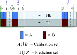
As abovementioned, the absorption of other components in the blood can affect the prediction of the target component. According to the “M + N” theory, the negative effect can be reduced by modeling. In this section, the calibration set selection considered not only the distribution of the target component (hemoglobin), but also the distribution of the non-target component (the total protein). The process is described as follows. First, the samples were sorted in an ascending order based on the concentration of hemoglobin. The sorted samples were divided into 19 intervals, with 4 samples in each interval. Two samples were selected from each interval as a calibration set. Second, the samples were sorted based on the total protein concentration. Then, the intervals were divided and the samples were selected for the calibration set in the same way. The union of these selected samples was regarded as the calibration set and the other samples were used for the prediction set. In this way, there were 11 samples in the prediction set and 66 samples in the training set. This method could ensure that the concentration of the hemoglobin and the total protein were uniformly distributed in the calibration set at the same time. Fig. 2 shows a schematic of the sample selection after sorting the samples on the basis of the concentration of the target component and non-target component.

Fig. 2 Schematic of the calibration set selection considering the concentration distributions of both the target and non-target components.

3. Experiment

3.1 Experimental section

Fig. 3 shows the schematic of the experimental apparatus configuration. It included the following devices: a light source, a spectrometer and a computer. As shown in Fig. 3, the DC regulated power supply HSPY-30-05 provided a direct current of 12 V. The broadband light of the halogen tungsten lamp went through the collimating lens, and then vertically irradiated on the tip of the finger. Fiber collected the transmitted light from the bottom of the finger and transferred the light to the spectrometer (AvaSpec-HS1024x58TEC), which had a spectral range from 200 nm to 1160 nm. The wavelength range used in this research was from 591 nm to 1120 nm. The spectrometer transferred the spectral data to the computer via USB.

Fig. 3 Schematic of the experimental apparatus configuration.

3.2 The samples and measurements

There were 77 subjects who took this test and acquired the spectral data. Table 1 shows the age distribution of the samples. Each subject placed their middle finger on the finger platform. They had to make sure that their finger pulps gently covered the detection optical fiber and the assembly remains stable. The integration time of the spectrometer was 20 ms and the test lasted for about 30 s. Therefore, for each subject, 1400 spectroscopic data were acquired. After the test, the subjects immediately got their blood examined to obtain the biochemical values.

Table 1 General information about the subjects

	Max age	Min age	Average age	Sample size
Male	66	24	38.05	40
Female	81	24	42.92	37

---

3.3 Extraction method of the dynamic spectrum

The dynamic spectrum of each sample was extracted by the single trial estimation method, which is one of the most mature extraction methods of the dynamic spectra.^25,26 The extracted dynamic spectra were normalized before modeling.

Fig. 4 shows a dynamic spectrum extracted by the single trial estimation method.

Fig. 4 Dynamic spectrum of one sample.

3.4 Assessment of the robustness of the model

This research predicted the hemoglobin concentration with the PLSR (partial least squares regression) method, which is commonly used in the dynamic spectrum analysis. This research considered the correlation coefficient of the calibration set R_c, the root mean square error of the calibration set RMSEC, the correlation coefficient of the prediction set R_p, and the root mean square error of the prediction set RMSEP as the parameters for the evaluation of model reliability.

4. Results and discussion

However, PLSR models with three different calibration sets selected by three different methods were established. Table 2 and Fig. 5 show the prediction results of the calibration models with samples selected by the three methods. The correlation coefficient R_c and RMSEC of the three calibration models were similar. However, it was obvious that the prediction result of the calibration model with the samples selected by the random selection method was very poor, with a 0.5388 correlation coefficient R_p and 15.9624 RMSEP value. Compared with the random selection method, the model with samples selected by the calibration set selection method considering the distribution of the hemoglobin concentration worked far better: the correlation coefficient R_p was 0.7998, which increased by 48.44%, and the RMSEP value was 13.4597, which reduced by 15.68%. Furthermore, the performance of the model, with the samples selected by the calibration set selection method that considers both the distribution of hemoglobin concentration and the total protein concentration, was the best: the R_p was 0.8640, increased by 60.36%, which was 8.03% more than that of the two abovementioned methods; the RMSEP value was 11.3858, reduced by 28.67%, which was 15.41% more than that of the two abovementioned methods.

Table 2 Comparison of the prediction results of the three methods

Method	Number of primary factor	Calibration set		Prediction set
		Rm	RMSEM (g L^−1)	Rp	RMSEP (g L^−1)
Random selection	5	0.8584	12.1716	0.5388	15.9624
Target component selection	5	0.8361	12.4705	0.7998	13.4597
Two components selection	5	0.8291	12.9914	0.8640	11.3858

---

Fig. 5 Prediction results of the three methods. (A) Random selection method. (B) Selection method based on the target component. (C) Selection method based on two components.

Obviously, the random selection method could not ensure that the concentration distribution of the samples in the calibration set completely covered that of the samples in the prediction set; thus, the model could have a low accuracy and a large error. Choosing samples of the calibration set according to the concentration distribution of the target component significantly improved the prediction ability of the model. The improvement of the prediction accuracy proved the feasibility of this method. Considering the effect of the non-target components, the proposed novel method selected the samples based on the concentration distribution of both the target component and non-target components. Thus, the method ensured not only the concentration distribution of the target component but also that of the non-target components of the calibration set and covered that of the samples in the prediction set. The performance of the calibration model with samples selected by the proposed selection method was the best. The modeling results demonstrated that the non-target components would affect the prediction accuracy of the target components and further confirmed the feasibility of the “M + N” theory.

5. Conclusion

The selection of a calibration set is very important for the reliability of the model. Also, the “M + N” theory is devoted to improve the robustness of a quantitative model for composition analysis with spectral data. In this study, based on “M + N” theory, we proposed a new calibration set selection method, which considered both the concentration distribution of the target and non-target components. The method was applied for the prediction of hemoglobin by the PLSR model using the DS method. The total protein, the most important component in the blood after hemoglobin, was regarded as the non-target component. The experimental results showed that the new selection method could significantly improve the model accuracy. It proved that the “M + N” theory plays a guiding role in the component analysis based on the spectral analysis by contrast experimentation. This research provided a new idea to improve the prediction performance of the model for composition analysis. This method can not only be used for noninvasive measurement, but can also play an important role in other chemical composition analysis when the measured object contains a variety in its composition. In the follow-up study, more components will be considered in the modeling system to improve the model robustness.

Acknowledgements

This study was supported by the Tianjin Application Basis & Front Technology Study Programs (no. 14JCZDJC33100).

Notes and references

1. S. R. Delwiche and R. A. Graybosch, Talanta, 2016, 146, 496–506.
2. P. H. Fidêncio, R. J. Poppi and J. C. de Andrade, et al., Commun. Soil Sci. Plant Anal., 2002, 33(9), 1607–1615.
3. J. Sundaram, C. V. Kandala and K. N. Govindarajan, et al., J. Sens. Technol., 2012, 2, 1–7.
4. G. Bázár, R. Romvári and A. Szabó, et al., Food Chem., 2016, 194, 873–880.
5. K. Maruo and Y. Yamada, J. Biomed. Opt., 2015, 20(4), 047003.
6. S. Liakat, K. A. Bors and T. Y. Huang, et al., Biomed. Opt. Express, 2013, 4(7), 1083–1090.
7. J. Kraitl, H. Ewald and H. Gehring, J. Opt. A: Pure Appl. Opt., 2005, 7(6), S318–S324.
8. C. E. F. D. Amaral and B. Wolf, Nat. Neurosci., 2008, 30(5), 541–549.
9. P. Bansod and M. C. Shrivastava, IETE Technical Review, 2015, 21(1), 45–54.
10. G. Li, Y. Wang and L. Lin, et al., Engineering in Medicine and Biology Society, 2005. Ieee-Embs 2005. International Conference of the IEEE, 2005, pp. 1960–1963.
11. H. Wang, G. Li and Z. Zhao, et al., Trans. Inst. Meas. Control, 2013, 35(35), 16–24.
12. G. Li, M. Zhou and L. Lin, Opt. Quantum Electron., 2014, 46(5), 691–698.
13. Y. J. Zhang, W. Z. Liu and X. H. Fu, et al., Spectrosc. Spectral Anal., 2015, 35(7), 1802–1807.
14. C. Tao and E. Martin, J. Chemom., 2007, 21(5–6), 198–207.
15. T. Talukdar, J. H. Moore and S. G. Diamond, J. Biomed. Opt., 2013, 18(5), 56001.
16. R. Maclin and D. Opitz, in Proceedings of the Fourteenth National Conference on Artificial Intelligence, 1998, pp. 546–551.
17. D. Xiang, M. Konigsberger and B. Wabuyele, et al., Analyst, 2009, 134(7), 1405–1415.
18. Z. Wu, C. Sui and X. Bing, et al., J. Pharm. Biomed. Anal., 2013, 77, 16–20.
19. X. Zhu, S. Yang and G. Li, et al., Spectrochim. Acta, Part A, 2009, 74(2), 344–348.
20. L. I. Gang, L. I. Zhe and X. F. Wang, et al., The Journal of Beijing Information Science and Technology University, 2013, 28(2), 9–13.
21. H. Liu, M. Wang and X. Li, et al., Anal. Methods, 2016, 8(23), 4648–4658.
22. G. Li, Y. S. Luo and Z. Li, et al., RSC Adv., 2016, 6, 38849–38854.
23. G. Li, Z. Zhao and L. Lin, et al., Spectrosc. Spectral Anal., 2012, 32(8), 2286–2289.
24. L. I. Gang, L. I. Zhe and L. I. Xiao-Xia, et al., Spectrosc. Spectral Anal., 2013, 33(6), 1456–1461.
25. L. I. Gang, C. Xiong and H. Q. Wang, et al., Guangpuxue Yu Guangpu Fenxi, 2011, 31(7), 1857–1861.
26. X. Li, G. Li and L. Lin, et al., Proc. SPIE, 2005, 5630, 688–696.

---