DOI:
10.1039/C6RA04345C
(Paper)
RSC Adv., 2016,
6, 52587-52595
Machine-learning prediction of the d-band center for metals and bimetals
Received
18th February 2016
, Accepted 23rd May 2016
First published on 25th May 2016
Abstract
The d-band center for metals has been widely used in order to understand activity trends in metal-surface-catalyzed reactions in terms of the linear Brønsted–Evans–Polanyi relation and Hammer–Nørskov d-band model. In this paper, the d-band centers for eleven metals (Fe, Co, Ni, Cu, Ru, Rh, Pd, Ag, Ir, Pt, Au) and their pairwise bimetals for two different structures (1% metal doped- or overlayer-covered metal surfaces) are statistically predicted using machine learning methods from readily available values as descriptors for the target metals (such as the density and the enthalpy of fusion of each metal). The predictive accuracy of four regression methods with different numbers of descriptors and different test-set/training-set ratios are quantitatively evaluated using statistical cross validations. It is shown that the d-band centers are reasonably well predicted by the gradient boosting regression (GBR) method with only six descriptors, even when we predict 75% of the data from only 25% given for training (average root mean square error (RMSE) < 0.5 eV). This demonstrates a potential use of machine learning methods for predicting the activity trends of metal surfaces with a negligible CPU time compared to first-principles methods.
Introduction
The ultimate goal in catalytic science is to accurately predict trends in catalytic activity using the electronic structure of metals, which will allow the rational design of surfaces with specific catalytic properties without extensive trial-and-error experiments. A semi-quantitative understanding of these trends is given by the d-band model of Nørskov and co-workers who defined the energy of the d-band center (εd) relative to the Fermi level (EF), εd–EF, as a function of the electronic structure of the metals.1–6 Assuming that the d-electrons of transition metals play a central role in chemisorption, they calculated the d-band center (εd–EF) for various metals using density functional theory (DFT) as an indicator to explain the adsorption energy trends for a given adsorbate: the higher the d-states are in energy relative to the Fermi level, the more empty the anti-bonding states and the larger the adsorption energy (strong bonding between the adsorbate and metal surface). This model was then verified with experimental and theoretical studies by various research groups.7–12 In a reaction on metal surfaces, strong binding of an intermediate will lead to surface poisoning, whereas weak binding will lead to a limited availability of the intermediate. In both cases, catalytic rates are less than optimal (Sabatier principle). Consequently, the catalytic activity of metals can show a so-called “volcano-type” dependence on the d-band center. Experimental data in some electrocatalytic and catalytic studies showed good correlation between the catalytic activity and the d-band center.1–3,9–15
Machine learning (ML) methods16–19 are being increasingly used in molecular science18,19 and materials science.20–24 In the ML framework, predictive computations are modeled as a function from some inputs to the output of desired values. Supervised ML methods statistically infer the function, given instances of input–output pairs called the training set: they inductively learn, from data, the underlying principle for input–output dependencies. Since ML methods are general-purpose, first-principles-free, and fully data-driven as such, they are widely applicable to prediction of various kinds of physical properties that have unknown or too complex principles to mathematically model.20–24 Considering that first-principles calculations are too time-consuming to explore the full spectrum of possibilities, and on the other hand, a great amount of data is being generated and accumulated in the field, ML methods can give a fast and high-precision alternative to the first-principles models. However, ML methods in catalysis25–34 are still in their infancy.
In order to demonstrate the potential use of ML methods in catalysis, we report herein the ML-based prediction of d-band center for metals and bimetallic compounds. Using the DFT method, Nørskov's group1,2 first calculated the d-band centers for 11 kinds of metals (Fe, Co, Ni, Cu, Ru, Rh, Pd, Ag, Ir, Pt, Au) and their 110 pairwise bimetals with two different structures (surface impurities and overlayers on clean metal surfaces).6 As seen in this case, the d-band centers are calculated by first principles independently for each metal or bimetal in conventional situations. In contrast, this paper quantitatively investigates a fully data-driven approach based on ML that infers the d-band center of a metal or a bimetal from those of some other metals and bimetals. For example, questions such as whether or not the d-band center of Cu–Co can be somehow inferred from those of Cu, Au, Cu–Fe, Ni–Ru, Pd–Co, and Rh–Pd would be of great interest from a materials informatics perspective. Our result shows sufficient predictability of d-band center by ML methods using a small set of readily available properties of metals as descriptors. Given the rapid growth of various data in recent years, this would suggest the promising role of ML methods that bypass or complement the first-principles calculations.
Methods and data
Dataset and descriptors
To assess the accuracy of ML predictions, we use the data of the d-band center (εd) relative to the Fermi level (EF), εd–EF, for 11 metals (Fe, Co, Ni, Cu, Ru, Rh, Pd, Ag, Ir, Pt, Au) and all pairwise bimetallic alloys (110 pairs of a host metal Mh and a guest metal Mg). These values are obtained in the DFT study by Nørskov et al.1,2 for two different structures of the surface impurities (Table 1) and overlayers (Table 2). In the original tables, the d-band centers for bimetals are given as shifts relative to the clean metal values, and they are converted to the values relative to the Fermi level. For Table 1, the surfaces considered are the most closely packed, and 1% guest metals are doped on the surface of the host metals. For Table 2, the overlayer structures are pseudomorphic, and the monolayers of guest metals are formed on the surface of the host metals. Although the two structures are physically very different, the Pearson's correlation coefficient between Tables 1 and 2 is 0.948 (p < 0.001) and the d-band centers are highly correlated. Therefore in order to differentiate these structure-specific values, any data-driven prediction requires a highly adaptive mechanism that can capture this subtle difference.
Table 1 DFT calculated d-band centers (eV) of metals (italic) and 1% guest metals (Mg) doped in the surface of host metals (Mh) as reported by Nørskov's group1,2
| Mh |
Mg |
| Fe |
Co |
Ni |
Cu |
Ru |
Rh |
Pd |
Ag |
Ir |
Pt |
Au |
| Fe |
−0.92 |
−0.87 |
−1.12 |
−1.05 |
−1.21 |
−1.46 |
−2.16 |
−1.75 |
−1.28 |
−2.01 |
−2.34 |
| Co |
−1.16 |
−1.17 |
−1.45 |
−1.33 |
−1.41 |
−1.75 |
−2.54 |
−2.08 |
−1.53 |
−2.36 |
−2.73 |
| Ni |
−1.20 |
−1.10 |
−1.29 |
−1.10 |
−1.43 |
−1.60 |
−2.26 |
−1.82 |
−1.43 |
−2.09 |
−2.42 |
| Cu |
−2.11 |
−2.07 |
−2.40 |
−2.67 |
−2.09 |
−2.35 |
−3.31 |
−3.37 |
−2.09 |
−3.00 |
−3.76 |
| Ru |
−1.20 |
−1.15 |
−1.40 |
−1.29 |
−1.41 |
−1.58 |
−2.23 |
−1.68 |
−1.39 |
−2.03 |
−2.25 |
| Rh |
−1.49 |
−1.39 |
−1.57 |
−1.29 |
−1.69 |
−1.73 |
−2.27 |
−1.66 |
−1.56 |
−2.08 |
−2.22 |
| Pd |
−1.46 |
−1.29 |
−1.33 |
−0.89 |
−1.59 |
−1.47 |
−1.83 |
−1.24 |
−1.30 |
−1.64 |
−1.66 |
| Ag |
−3.58 |
−3.46 |
−3.63 |
−3.83 |
−3.46 |
−3.44 |
−4.16 |
−4.30 |
−3.16 |
−3.80 |
−4.45 |
| Ir |
−1.90 |
−1.84 |
−2.06 |
−1.90 |
−2.02 |
−2.26 |
−2.84 |
−2.24 |
−2.11 |
−2.67 |
−2.85 |
| Pt |
−1.92 |
−1.77 |
−1.85 |
−1.53 |
−2.11 |
−2.02 |
−2.42 |
−1.81 |
−1.87 |
−2.25 |
−2.30 |
| Au |
−2.93 |
−2.79 |
−2.93 |
−3.01 |
−2.86 |
−2.81 |
−3.39 |
−3.35 |
−2.58 |
−3.10 |
−3.56 |
Table 2 DFT calculated d-band centers (eV) of metals (italic) and the surface monolayer of guest metals (Mg) on the surface of host metals (Mh) reported by Nørskov's group1,2
| Mh |
Mg |
| Fe |
Co |
Ni |
Cu |
Ru |
Rh |
Pd |
Ag |
Ir |
Pt |
Au |
| Fe |
−0.92 |
−0.78 |
−0.96 |
−0.97 |
−1.65 |
−1.64 |
−2.24 |
−2.17 |
−1.87 |
−2.40 |
−3.11 |
| Co |
−1.18 |
−1.17 |
−1.37 |
−1.23 |
−1.87 |
−2.12 |
−2.82 |
−2.53 |
−2.26 |
−3.06 |
−3.56 |
| Ni |
−0.33 |
−1.18 |
−1.29 |
−1.17 |
−1.92 |
−2.03 |
−2.61 |
−2.43 |
−2.15 |
−2.82 |
−3.39 |
| Cu |
−2.42 |
−2.29 |
−2.49 |
−2.67 |
−2.89 |
−2.94 |
−3.71 |
−3.88 |
−2.99 |
−3.82 |
−4.63 |
| Ru |
−1.11 |
−1.04 |
−1.12 |
−1.11 |
−1.41 |
−1.53 |
−1.88 |
−1.81 |
−1.54 |
−2.02 |
−2.27 |
| Rh |
−1.42 |
−1.32 |
−1.39 |
−1.51 |
−1.70 |
−1.73 |
−2.12 |
−1.81 |
−1.70 |
−2.18 |
−2.30 |
| Pd |
−1.47 |
−1.29 |
−1.29 |
−1.03 |
−1.94 |
−1.58 |
−1.83 |
−1.68 |
−1.52 |
−1.79 |
−1.97 |
| Ag |
−3.75 |
−3.56 |
−3.62 |
−3.68 |
−3.80 |
−3.63 |
−4.03 |
−4.30 |
−3.50 |
−3.93 |
−4.51 |
| Ir |
−1.78 |
−1.71 |
−1.78 |
−1.55 |
−2.12 |
−2.14 |
−2.53 |
−2.20 |
−2.11 |
−2.60 |
−2.70 |
| Pt |
−1.90 |
−1.72 |
−1.71 |
−1.47 |
−2.13 |
−2.01 |
−2.23 |
−2.06 |
−1.96 |
−2.25 |
−2.33 |
| Au |
−3.03 |
−2.82 |
−2.85 |
−2.86 |
−3.09 |
−2.89 |
−3.21 |
−3.44 |
−2.77 |
−3.13 |
−3.56 |
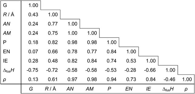
Regarding the choice of descriptors for metals, we pre-tested several candidates and chose nine physical properties (Table 3), which are readily available from the periodic table and a handbook.35 From a practical point of view, it is important to choose readily accessible but characteristic values as descriptors in order to effectively bypass time-consuming DFT calculations with keeping good prediction accuracy. Each metal can thus be represented as a 9-dimensional vector of the descriptor values. For prediction of the d-band center for bimetals made of Mh and Mg, an 18-dimensional concatenated vector of Mh and Mg is used. For monometallic surfaces, we use an 18-dimensional vector by concatenating two vectors of the same metal. Out of all 18 descriptors, we also search for smaller subsets of descriptors yielding simpler models by assessing the relevance or redundancy of each descriptor. Table 4 shows the correlation matrix between descriptors, and we observe highly correlated variables of descriptors. This motivates us to investigate variable selection to find a smaller non-redundant subset of 18 descriptors. Table 5 indicates the correlation coefficients between each descriptor and the d-band center. We observe that no single descriptors have direct correlation to the d-band centers.
Table 3 Input features (descriptors) used for prediction of d-band centers from ref. 34a
| Metal |
G |
R/Å |
AN |
AM/g mol−1 |
P |
EN |
IE/eV |
ΔfusH/J g−1 |
ρ/g cm−3 |
| Group (G), bulk Wigner–Seitz radius (R) in Å, atomic number (AN), atomic mass (AM) in g mol−1, period (P) electronegativity (EN), ionization energy (IE) in eV, enthalpy of fusion (ΔfusH) in J g−1, density at 25 °C (ρ) in g cm−3. |
| Fe |
8 |
2.66 |
26 |
55.85 |
4 |
1.83 |
7.90 |
247.3 |
7.87 |
| Co |
9 |
2.62 |
27 |
58.93 |
4 |
1.88 |
7.88 |
272.5 |
8.86 |
| Ni |
10 |
2.60 |
28 |
58.69 |
4 |
1.91 |
7.64 |
290.3 |
8.90 |
| Cu |
11 |
2.67 |
29 |
63.55 |
4 |
1.90 |
7.73 |
203.5 |
8.96 |
| Ru |
8 |
2.79 |
44 |
101.07 |
5 |
2.20 |
7.36 |
381.8 |
12.10 |
| Rh |
9 |
2.81 |
45 |
102.91 |
5 |
2.28 |
7.46 |
258.4 |
12.40 |
| Pd |
10 |
2.87 |
46 |
106.42 |
5 |
2.20 |
8.34 |
157.3 |
12.00 |
| Ag |
11 |
3.01 |
47 |
107.87 |
5 |
1.93 |
7.58 |
104.6 |
10.50 |
| Ir |
9 |
2.84 |
77 |
192.22 |
6 |
2.20 |
8.97 |
213.9 |
22.50 |
| Pt |
10 |
2.90 |
78 |
195.08 |
6 |
2.20 |
8.96 |
113.6 |
21.50 |
| Au |
11 |
3.00 |
79 |
196.97 |
6 |
2.40 |
9.23 |
64.6 |
19.30 |
Table 4 The correlation matrix of 9 descriptors for 11 metals in Table 3
Table 5 The correlation coefficients between each of 18 descriptors and the d-band center
| |
G |
R/Å |
AN |
AM |
P |
EN |
IE |
ΔfusH |
ρ |
| (For host metal) |
| Impurities |
−0.63 |
−0.53 |
−0.29 |
−0.29 |
−0.26 |
−0.02 |
−0.15 |
0.56 |
−0.17 |
| Overlayers |
−0.63 |
−0.34 |
−0.11 |
−0.11 |
−0.06 |
0.13 |
−0.06 |
0.49 |
0.00 |
![[thin space (1/6-em)]](https://www.rsc.org/images/entities/char_2009.gif) |
| (For guest metal) |
| Impurities |
−0.24 |
−0.35 |
−0.26 |
−0.26 |
−0.27 |
−0.28 |
−0.24 |
0.33 |
−0.20 |
| Overlayers |
−0.22 |
−0.47 |
−0.41 |
−0.40 |
−0.42 |
−0.39 |
−0.31 |
0.36 |
−0.33 |
Monte Carlo cross validation for assessing predictability
Our primary interest is data-driven prediction of the d-band center of X from the d-band centers of other metals and bimetals than X. In order to evaluate this aspect, we first separate 121 targets (11 metals and 110 bimetals) into two disjoint sets of “test set” of size n and “training set” of size 121-n. Then our problem is to evaluate how accurately the d-band centers of the test set can be predicted by using those of the training set. First, an ML model is build using the training set. Then, using that model, the d-band centers of the test set are predicted, and their root mean square error (RMSE) between the predicted values and true values (ground truth) is calculated for predictability evaluation. A single-shot trial of this procedure gives an estimate of RMSE, but if we change the split of training and test sets, the estimate would vary with a certain level of variance. For quantitative evaluation, we reduce this estimation variance by repeating the single-shot trial over 100 random test/training splits, i.e., 100 random leave-n-out trials, and use the mean of 100 RMSE estimates as the prediction accuracy of the ML model. The test set in each trial is never used to build the corresponding ML model in that trial, and simulates yet-unseen targets to be predicted. Another benefits is that we can also control the size n of test set, and analyze how large training set is required for accurate prediction. Note that this method is well established in statistics, and called Monte Carlo cross validation,36 or other various names such as leave-n-out,20,37 random permutation cross validation (shuffle and split),38 and random subsampling cross validation.39 This method is used in related work,20 and also well matched to our scenario than typical choices such as k-fold cross validation and bootstrapping.
Machine learning methods and tuning parameter selection
For ML methods, we use two linear and two nonlinear regression methods (Table 6). The models selected here are the most commonly used in the ML field, the details about individual methods are found in standard ML textbooks.16,40 The software implementations of these algorithms are also available as many off-the-shelf packages. In this paper, we use a widely used package, scikit-learn (http://scikit-learn.org).38 In practice, besides the target parameters to be estimated from the training set, some models also have tuning parameters that need to be set before training, and appropriate setting of this parameter is the key to the success in prediction. For those tuning parameters, we tested a reasonable range of candidate values in an exhaustive way (grid search), and chose the best parameter by 3-fold cross validation on the training set. The tested ranges of values are also indicated in Table 6. Note that the test data should never be used to select a tuning parameter.
Table 6 List of the regression methods
| Abbreviation |
Method |
Tuning parameters [tested range] |
| Linear methods |
| OLS |
Ordinary least squares regression |
(No tuning parameters) |
| PLS |
Partial least squares regression |
n_components ∈ [1,2,…,# of vars] |
![[thin space (1/6-em)]](https://www.rsc.org/images/entities/char_2009.gif) |
| Nonlinear methods |
| GPR |
Gaussian process regression |
Theta0 ∈ [1.0,10−1,10−2,10−3,10−4,10−5] |
| GBR |
Gradient boosting regression |
Learning_rate ∈ [1.0,10−1,10−2,10−3,10−4,10−5] |
| Max_depth ∈ [4,6,8,10] |
n_estimators ∈ [100![[thin space (1/6-em)]](https://www.rsc.org/images/entities/char_2009.gif) 250 250![[thin space (1/6-em)]](https://www.rsc.org/images/entities/char_2009.gif) 500] 500] |
Results and discussion
Screening of predictive ML methods
For prediction of d-band center for the surface impurities (Table 1), we performed parameter fitting by the four ML methods in Table 6: two linear methods, ordinary least-squares regression (OLS) and partial least-squares regression (PLS), and two nonlinear methods, Gaussian process regression (GPR) and gradient boosting regression (GBR). OLS is the most basic method and gives a stable baseline performance. For higher-dimensional data, the data distribution often lies in a lower-dimensional subspace due to the correlation between descriptors. Statistically decorrelating the descriptors, PLS performs OLS on an identified lower-dimensional subspace. In addition to these conventional linear methods, we also investigated two nonlinear methods, GPR and GBR. Among the various nonlinear methods we pre-tested, GPR and GBR showed two of the best prediction performances. GPR is one of the most common methods for the prediction of continuous values; it is based on kernel methods, which gives a flexible model for the data. GBR41 is another popular choice as it is widely used and performs well in the top-level data prediction competitions such as kaggle in recent years;42,43 Technically, it is an ensemble model of boosted regression trees, which often gives accurate and stable predictions.
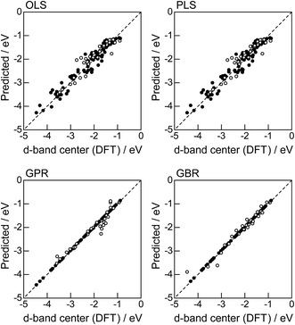
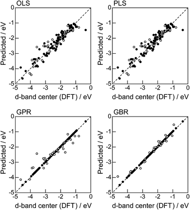
In order to evaluate the predictive capability of the ML models, we use Monte Carlo cross validation with random leave-25%-out for Table 1: assuming that 25% of Table 1 is not yet obtained, ML methods infer those values statistically using other 75% available values. Fig. 1 illustrates the predictive performance of the four ML methods in a single-shot random trial with 75% training set (●) and 25% test set (○). This case uses all 18 descriptors, 9 for the host and 9 for the guest metal. The X-axis represents the DFT calculated d-band center (ground truth), and the Y-axis gives the value predicted by the ML methods. The deviation from the X = Y line indicates the error in prediction. Clearly, the test set (○) of the linear models (OLS and PLS) show larger deviations than the nonlinear models (GPR and GBR), and those of the GBR model shows the least deviation from the line. Note that PLS is best performed when it is identical to OLS, this implies that linear dimensional reduction does not work for this problem.
 |
| | Fig. 1 DFT calculated local d-band center for metals and 1% guest metal-doped metals (Table 1) and the values predicted by linear (OLS, PLS) and nonlinear regression (GPR, GBR): (●) training set = 75%, (○) test set = 25%. | |
For more quantitative evaluation, we perform 100 random trials of this single-shot leave-25%-out. The root mean square error (RMSE) of the difference between the predicted values and the ground truth is calculated for each trial, and averaged to obtain the mean RMSE values and their standard deviations. As seen in Table 7, the mean RMSE values of the linear models, OLS (0.26 ± 0.03 eV for test) and PLS (0.26 ± 0.03 eV for test), are larger than those of the nonlinear models, GPR (0.21 ± 0.05 eV for test) and GBR (0.17 ± 0.04 eV for test), suggesting that the nonlinear models are more accurate than the linear models. Of the two nonlinear models, the RMSE for prediction using GBR was smaller than that from GPR. From these results, we concluded that GBR would be the best choice for the prediction of the d-band centers for the surface impurities (Table 1). It is known that the GBR model has a higher flexibility than the linear regression models and a higher stability than the GPR model that is more sensitive to the tuning-parameter settings. It should be noted that linear models have less standard deviations than nonlinear models. Linear models are less flexible but usually more stable than nonlinear models, and this tradeoff needs to be considered in accordance with the intended use.
Table 7 The mean RMSEs of each method with 18 descriptors (over 100 of leave-25%-out)
| |
Impurities |
Overlayers |
| Training error |
Test error |
Training error |
Test error |
| Mean |
sd |
Mean |
sd |
Mean |
sd |
Mean |
sd |
| (min, max) |
(min, max) |
(min, max) |
(min, max) |
| OLS |
0.20 |
0.01 |
0.26 |
0.03 |
0.27 |
0.02 |
0.34 |
0.05 |
| (0.17, 0.23) |
(0.18, 0.33) |
(0.24, 0.31) |
(0.22, 0.48) |
| PLS |
0.20 |
0.01 |
0.26 |
0.03 |
0.27 |
0.02 |
0.34 |
0.05 |
| (0.17, 0.23) |
(0.18, 0.33) |
(0.24, 0.31) |
(0.22, 0.48) |
| GPR |
0.00 |
0.00 |
0.21 |
0.05 |
0.00 |
0.00 |
0.35 |
0.07 |
| (0.00, 0.00) |
(0.13, 0.36) |
(0.00, 0.00) |
(0.18, 0.53) |
| GBR |
0.00 |
0.00 |
0.17 |
0.04 |
0.00 |
0.00 |
0.19 |
0.04 |
| (0.00, 0.00) |
(0.10, 0.34) |
(0.00, 0.00) |
(0.09, 0.29) |
Evaluations of descriptor importance for GBR prediction
Next, we investigated the relevance or redundancy of each of the 18 descriptors in Table 3, which were used in the GBR model. GBR is based on an ML technique called “boosting”, it adaptively combine large numbers of relatively simple regression-tree models that recursively partition the data by a single selected descriptor. Thus it provides a feature-importance score for each descriptor: a weighted average of the number of times the descriptor is selected for partitioning. This score can be used to assess the relative importance of that descriptor with respect to the predictability of the d-band center values. Note that these results are valid only for GBR, and the statistical importance of descriptors may vary with the ML method used.
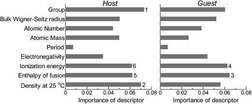
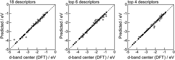
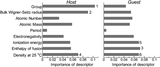
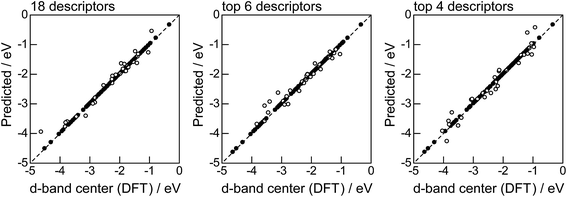
Fig. 2 shows the feature-importance scores of all 18 descriptors for predicting Table 1. The 6 most important descriptors are highlighted with a rank next to their bars. These were (1) the group in the periodic table for the host metal, (2) the density at 25 °C for the host metal, (3) the enthalpy of fusion for the guest metal, (4) the ionization energy for the guest metal, (5) the enthalpy of fusion for the host metal, and (6) the ionization energy for the host metal. To evaluate the effect of the number of descriptors on the predictive performance of GBR, the prediction results with 18 (all), the top 6 and the top 4 descriptors are compared as shown in Fig. 3. For quantitative evaluation, we also repeated the tests in Fig. 3 100 times with random splits, and calculated the mean RMSEs for prediction. The resultant values were 0.17 ± 0.04 eV with 18 descriptors, 0.18 ± 0.04 eV with the top 6 descriptors, and 0.16 ± 0.04 eV with the top 4 descriptors. As a result, the ML prediction performance for the 1% guest metal-doped metals (Table 1) remained the same good level even when we use only 4 descriptors. Furthermore we observed that the prediction accuracy with 6 descriptors were better than with 4 descriptors when we increased the test set from 25% to a higher percentage. Thus we used the GBR model with the top 6 descriptors for the subsequent analysis.
 |
| | Fig. 2 Feature-importance scores of the descriptors (Table 3) for the GBR prediction of the d-band centers for metals and 1% guest metal-doped metals (Table 1). | |
 |
| | Fig. 3 DFT calculated local d-band center for metals and 1% guest metal-doped metals (Table 1) correlated with the values predicted by GBR with the 18 (all), top 6, and top 4 descriptors in Fig. 2: (●) training set = 75%, (○) test set = 25%. | |
Model estimation using a different ratio of test/training splits
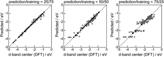
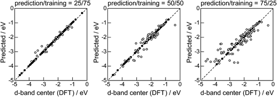
Lastly, we investigated how large training set is required for ML to achieve sufficient prediction performance. Fig. 4 shows the predictive performance using GBR with the top 6 descriptors for different ratios of the test/training sets, 25%/75%, 50%/50%, and 75%/25%. For Table 1, we have 121 values in total, and 25%/75% corresponds to sets of size 30/91, 50%/50% to 61/60, and 25%/75% to 90/31. For quantitative evaluation, we also calculated the mean RMSEs for the 100 random splits for each setting: the resultant values were 0.18 ± 0.04 eV for the 25%/75% test, 0.23 ± 0.05 eV for the 50%/50% test, and 0.38 ± 0.07 eV for the 75%/25% test. These results quantitatively showed a general trend of ML where the more data we have, the better we get, and also showed that we can predict the d-band center for the surface impurities (Table 1) with a moderate level of accuracy (RMSE = 0.38 ± 0.07 eV) even when only 25% of the data are available and 75% are missing. This result provides a useful guideline for the trade-off between the predictive performance and data availability.
 |
| | Fig. 4 DFT calculated local d-band center for 1% guest metals on the surface of host metals and the values predicted by GBR with the top 6 descriptors: (●) training set, (○) test set. | |
Prediction of d-band centers for surface overlayers on metal surfaces
The evaluation procedure used for the 1% guest-doped cases (Table 1, Fig. 1–4) were also applied to the prediction of d-band center for surface overlayers on different metal surfaces (Table 2), and the corresponding results were shown in Fig. 5–8, respectively. Similar to the results in Fig. 1, the comparison of the four ML methods with the 18 descriptors (Fig. 5) showed that the predictions with GBR were better than with the other methods; the mean RMSEs for the 100 random 75%/25% splits were 0.34 ± 0.05 eV for OLS, 0.34 ± 0.05 eV for PLS, 0.35 ± 0.07 eV for GPR, and 0.19 ± 0.04 eV for GBR (Table 7). Both GPR and GBR achieve the training error of 0.00 as seen in Table 7, but due to the high dependency on tuning parameter setting, GPR fails to predict the test set. GPR would also perform well when the tuning parameter (set by 3-fold cross validation on the training set) fits into the test data, but this is not the case in general. In actual, we observe in Table 7 that GPR has larger estimation variance than any other methods as shown in the sd values for test. In contrast, GBR has a less tuning parameter dependency and also perform well for the test set. Thus again, we adopted GBR for further analysis. Fig. 6 shows the feature-importance scores of all 18 descriptors for predicting Table 2. The top 6 descriptors were (1) the group in the periodic table for the host metal, (2) the bulk Wigner–Seitz radius for the host metal, (3) the enthalpy of fusion for the guest metal, (4) the density at 25 °C for the host metal, (5) the ionization energy for the guest metal, and (6) the density at 25 °C for the guest metal. Using GBR with 18 (all), the top 6, and the top 4 descriptors for 75%/25% splits, the mean RMSE for the 100 random splits were 0.19 ± 0.04 eV with 18 descriptors, 0.19 ± 0.04 eV with the top 6 descriptors, and 0.23 ± 0.05 eV with the top 4 descriptors. Hence GBR with the top 6 descriptors kept the same best prediction performance as GBR with all 18 descriptors. Using GBR with the top 6 descriptors, we evaluated the predictive performance for different ratios, 25%/75%, 50%/50%, and 75%/25%, of the test/training sets (Fig. 8). The mean RMSEs for the 100 random splits were 0.19 ± 0.04 eV for the 25%/75% test, 0.27 ± 0.05 eV for the 50%/50% test, and 0.41 ± 0.08 eV for the 75%/25% test. From these results, we can conclude that the d-band centers for the surface overlayers (Table 2) can be predicted by the GBR method using 6 descriptors with a moderate accuracy (RMSE = 0.41 ± 0.08 eV), even when only 25% of the data are available and 75% are missing.
 |
| | Fig. 5 DFT calculated local d-band center for the surface monolayer of guest metals on the host metals (Table 2) and the predicted values from linear (OLS, PLS) and nonlinear (GPR, GBR) regression methods: (●) training set = 75%, (○) test set = 25%. | |
 |
| | Fig. 6 Feature-importance scores of the descriptors for the GBR prediction of the d-band centers for the surface monolayer of guest metals on the host metals. | |
 |
| | Fig. 7 DFT calculated local d-band center for the surface monolayer of guest metals on the host metals (Table 2) and the values predicted by GBR with the 18 (all), top 6, and top 4 descriptors in Fig. 6: (●) training set = 75%, (○) test set = 25%. | |
 |
| | Fig. 8 DFT calculated local d-band center for the surface monolayer of guest metals on the host metals (Table 2) and the values predicted by GBR with the top 6 descriptors: (●) training set, (○) test set. | |
Conclusion
The d-band center for surfaces of monometallic (Fe, Co, Ni, Cu, Ru, Rh, Pd, Ag, Ir, Pt, Au) surfaces and bimetallic surfaces with two different structures (surface impurities and overlayers on clean metal surfaces)1,2 can be reasonably well predicted by a machine learning method (GBR method) using at most 6 readily available descriptors. Our results demonstrate a potential use of machine learning methods in catalysts design, suggesting a data-driven approach with a negligible CPU time compared to the first-principles models.
Acknowledgements
This work was supported in part by JSPS/MEXT Kakenhi 26120503, 26330242, 15H05711, Grant-in-Aid for Scientific Research on Innovative Areas “Nano Informatics” (25106010) from JSPS/MEXT “Elements Strategy Initiative to Form Core Research Center”, JST PRESTO, JST CREST, JST ERATO, RIKEN PostK, and NIMS MI2I.
References
- B. Hammer and J. K. Nørskov, Adv. Catal., 2000, 45, 71–129 CAS.
- A. Ruban, B. Hammer, P. Stoltze, H. L. Skriver and J. K. Nørskov, J. Mol. Catal. A: Chem., 1997, 115, 421–429 CrossRef CAS.
- J. K. Nørskov, T. Bligaard, J. Rossmeisl and C. H. Christensen, Nat. Chem., 2009, 1, 37–46 CrossRef PubMed.
- J. K. Nørskov, F. Abild-Pedersen, F. Studt and T. Bligaard, Proc. Natl. Acad. Sci. U. S. A., 2011, 108, 937–943 CrossRef PubMed.
- H. Toulhoat and P. Raybaud, J. Catal., 2003, 216, 63–72 CrossRef CAS.
- A. Vojvodic, J. K. Nørskov and F. Abild-Pedersen, Top. Catal., 2014, 57, 25–32 CrossRef CAS.
- C. Lu, I. C. Lee, R. I. Masel, A. Wieckowski and C. Rice, J. Phys. Chem. A, 2002, 106, 3084–3091 CrossRef CAS.
- M. K. Sabbe, L. Laín, M. Reyniers and G. B. Marin, Phys. Chem. Chem. Phys., 2013, 15, 12197–12214 RSC.
- H. Abe, H. Yoshikawa, N. Umezawa, Y. Xu, G. Saravanan, G. V. Ramesh, T. Tanabe, R. Kodiyath, S. Ueda, N. Sekido, Y. Yamabe-Mitarai, M. Shimoda, T. Ohno, F. Matsumoto and T. Komatsu, Phys. Chem. Chem. Phys., 2015, 17, 4879–4887 RSC.
- Y. Jiao, Y. Zheng, M. Jaroniec and S. Z. Qiao, Chem. Soc. Rev., 2015, 44, 2060–2086 RSC.
- F. Calle-Vallejo and M. T. M. Koper, Electrochim. Acta, 2012, 84, 3–11 CrossRef CAS.
- S. Furukawa, K. Ehara, K. Ozawa and T. Komatsu, Phys. Chem. Chem. Phys., 2014, 16, 19828–19831 RSC.
- R. Y. Zheng, M. P. Humbert, Y. X. Zhu and J. G. Chen, Catal. Sci. Technol., 2011, 1, 638–643 CAS.
- M. Tamura, K. Kon, A. Satsuma and K. Shimizu, ACS Catal., 2012, 2, 1904–1909 CrossRef CAS.
- N. Acerbi, S. C. E. Tsang, G. Jones, S. Golunski and P. Collier, Angew. Chem., Int. Ed., 2013, 52, 7737–7741 CrossRef CAS PubMed.
- K. Murphy, Machine Learning: a Probabilistic Perspective, The MIT Press, 2012 Search PubMed.
- F. Pedregosa, G. Varoquaux, A. Gramfort, V. Michel, B. Thirion, O. Grisel, M. Blondel, P. Prettenhofer, R. Weiss, V. Dubourg, J. Vanderplas, A. Passos, D. Cournapeau, M. Brucher, M. Perrot and E. Duchesnay, J. Mach. Learn. Res., 2011, 12, 2825–2830 Search PubMed.
- K. Hansen, G. Montavon, F. Biegler, S. Fazli, M. Rupp, M. Scheffler, O. A. von Lilienfeld, A. Tkatchenko and K.-R. Müller, J. Chem. Theory Comput., 2013, 9, 3404–3419 CrossRef CAS PubMed.
- M. Rupp, A. Tkatchenko, K.-R. Müller and O. A. von Lilienfeld, Phys. Rev. Lett., 2012, 108, 058301 CrossRef PubMed.
- L. Ghiringhelli, J. Vybiral, S. Levchenko, C. Draxl and M. Scheffler, Phys. Rev. Lett., 2015, 114, 105503 CrossRef PubMed.
- Y. Saad, D. Gao, T. Ngo, S. Bobbitt, J. R. Chelikowsky and W. Andreoni, Phys. Rev. B: Condens. Matter Mater. Phys., 2012, 85, 104104 CrossRef.
- A. Seko, T. Maekawa, K. Tsuda and I. Tanaka, Phys. Rev. B: Condens. Matter Mater. Phys., 2014, 89, 054303 CrossRef.
- K. Rajan, Annu. Rev. Mater. Res., 2015, 45, 153–169 CrossRef CAS.
- T. Le, V. C. Epa, F. R. Burden and D. A. Winkler, Chem. Rev., 2012, 112(5), 2889–2919 CrossRef CAS PubMed.
- Y. Okamoto, Chem. Phys. Lett., 2004, 395, 279–284 CrossRef CAS.
- K. Omata, Ind. Eng. Chem. Res., 2011, 50, 10948–10954 CrossRef CAS.
- G. Rothenberg, Catal. Today, 2008, 137, 2–10 CrossRef CAS.
- A. G. Maldonado and G. Rothenberg, Chem. Soc. Rev., 2010, 39, 1891–1902 RSC.
- E.-J. Ras, M. J. Louwerse and G. Rothenberg, Catal. Sci. Technol., 2012, 2, 2456–2464 CAS.
- E.-J. Ras, M. J. Louwerse, M. C. Mittelmeijer-Hazeleger and G. Rothenberg, Phys. Chem. Chem. Phys., 2013, 15, 8795–8804 RSC.
- E.-J. Ras and G. Rothenberg, RSC Adv., 2014, 4, 5963–5974 RSC.
- X. Ma, Z. Li, L. E. K. Achenie and H. Xin, J. Phys. Chem. Lett., 2015, 6, 3528–3533 CrossRef CAS PubMed.
- H. Xin, A. Holewinski and S. Linic, ACS Catal., 2012, 2, 12–16 CrossRef CAS.
- N. Madaan, N. R. Shiju and G. Rothenberg, Catal. Sci. Technol., 2016, 6, 125–133 Search PubMed.
- CRC Handbook of Chemistry and Physics, ed. D. R. Lide, CRC Press, London, 83rd edn, 2002 Search PubMed.
- R. R. Picard and R. D. Cook, J. Am. Stat. Assoc., 1984, 79(387), 575–583 CrossRef.
- J. Shao, J. Am. Stat. Assoc., 1993, 88(422), 486–494 CrossRef.
- F. Pedregosa, G. Varoquaux, A. Gramfort, V. Michel, B. Thirion, O. Grisel, M. Blondel, P. Prettenhofer, R. Weiss, V. Dubourg, J. Vanderplas, A. Passos, D. Cournapeau, M. Brucher, M. Perrot and E. Duchesnay, J. Mach. Learn. Res, 2011, 12, 2825–2830 Search PubMed.
- N. Japkowicz and M. Shah, Evaluating Learning Algorithms: A Classification Perspective, Cambridge University Press, 2011 Search PubMed.
- T. Hastie, R. Tibshirani, and J. Friedman, The Elements of Statistical Learning: Data Mining, Inference, and Prediction, Springer, 2013 Search PubMed.
- J. Friedman, Ann. Statist., 2001, 29(5), 1189–1232 CrossRef.
- T. Chen and T. He, JMLR. Workshop and Conference Proceedings, 2015, vol. 42, pp. 69–80 Search PubMed.
- T. Chen and C. Guestrin, arXiv:1603.02754, 2016.
|
| This journal is © The Royal Society of Chemistry 2016 |
Click here to see how this site uses Cookies. View our privacy policy here.  *ab,
Ken-ichi Shimizucd,
Koji Tsudaefg and
Satoru Takakusagic
![[thin space (1/6-em)]](https://www.rsc.org/images/entities/char_2009.gif)
![[thin space (1/6-em)]](https://www.rsc.org/images/entities/char_2009.gif)
![[thin space (1/6-em)]](https://www.rsc.org/images/entities/char_2009.gif) 250
250![[thin space (1/6-em)]](https://www.rsc.org/images/entities/char_2009.gif) 500]
500]